Spatial Embedding and Complexity: The Small World is Not Enough

Spatial Embedding and Complexity: The

Small-World is Not Enough

Christopher L. Buckley and Seth Bullock

School of Electronics and Computer Science, University of Southampton, UK

clb05r|[email protected]

Abstract. The “order for free” exhibited by some classes of system has been exploited by natural selection in order to build systems capable of exhibiting complex behaviour. Here we explore the impact of one or-dering constraint, spatial embedding, on the dynamical complexity of networks. We apply a measure of functional complexity derived from information theory to a set of spatially embedded network models in order to make some preliminary characterisations of the contribution of space to the dynamics (rather than mere structure) of complex systems. Although our measure of behavioural complexity hinges on a balance be-tween functional integration and segregation, which seem related to an understanding of the world property, we demonstrate that small-world structures alone are not enough to induce complexity. However, purely spatial constraints can produce systems of high intrinsic com-plexity by introducing multiple scales of organisation within a network.

1

Introduction

From its outset, artificial life has concentrated on how simple properties can give rise to complex organisation and behaviour. The interplay between, inter alia, non-linear, local interactions, physical constraints, noise, and processes of copy-ing or competitive exclusion have been shown to give rise to self-organisation, auto-catalysis, path dependence, and emergent behaviour in many different ways [1, 2]. For most complex systems, spatial embedding is a potential source of en-abling constraint. By projecting a system of interacting elements into a low dimensional space, local correlations are imposed and maintained. These cor-relations can predispose systems to exhibit behaviour that would otherwise be unstable [3].

were clearly required to combine their socialand geographical knowledge to meet this challenge.

Likewise, when Watts and Strogatz [4] went on to formalise the notion as the “small-world property”, they also made explicit use of spatial embedding. They construct a lattice where the pattern of connectivity reflects the regu-lar (isotropic, homogeneous) spatial organisation of the nodes, and find that repeated application of random rewiring events gradually erodes the spatial or-ganisation until a random graph results. Intermediate between the ordered lattice and the disordered random graph, Watts and Strogatz characterised small-world structures that simultaneously exhibit a small characteristic path length and a high degree of clustering.

Here we are interested in the relationship between spatial constraints, net-work topology, and functional complexity, an information-theoretic measure of which has been developed in order to characterise some important properties of both vertebrate and invertebrate nervous systems [5]. In particular, it has been used to identify, and quantify, a tension that lies at the heart of neural information processing. On the one hand, the brain must integrate distributed information in order to produce coherent behaviour, on the other, a great deal of experimental work demonstrates that neural regions specialise [6]. It has been suggested that a measure of complexity might reconcile the notions of neural segregation and integration within a single theoretical framework [5]. In partic-ular, biological networks have high complexity by this measure, which has been linked to spatial constraints on connectivity (along with other structural proper-ties, e.g., hierarchical organisation) [5]. Furthermore, it has been suggested that both the small-world property and high complexity are coincident in biological neural networks [7]. This paper examines these issues, first exploring the extent to which spatially constructed small worlds are associated with high complexity, and then assessing the more general impact of spatial embedding and spatial structure on network complexity.

2

The Complexity Measures

nervous system [8]. Note: even linear interactions between nodes can still give rise to interesting dynamics in large systems.

The level of dependence and independence between sets of elements in such a system can be measured through the concept of mutual information. Equa-tion (1) gives the mutual informaEqua-tion,M I(X), between the jth

of k subsets of

X and its complement X−Xk

j, in terms of the entropy, H(x). Entropy is de-rived from consideration of the covariance between the activity of each of the elements, denoted by the covariance matrixCOV which can be considered to quantify the dependence between each of the elements [5].

M I(Xk

j;X−X k

j) =H(X k

j) +H(X−X k

j)−H(X), (1)

H(X) = 0.5 ln((2πexp)n|COV_|)

An estimate of the integration (i.e., the shared information) between the elements of a subset is given by equation (2), which measures the difference between the sum of the deviations from independence of each element taken independently, and the entropy of the system as a whole.

I(X) =Σn

i=1H(xi)−H(x) (2) Integration is minimal where dependence between elements is uniform, and max-imal where the elements are highly and heterogeneously interdependent. Com-plexity is then given by equation (3), which measures the integration within network subsets of different sizes, denoted by k. Complexity is proportional to the difference between the average value of integration for a subsetXk

j (over all it j permutations) and the integration expected for a linear increase in system size summed over all subset sizes.

CN(X) =Σin=1[(k/n)I(X)−< I(X k

j)>] (3) Like other notions of complexity, this measure is low when either all elements are independent and hence completely segregated, or conversely, the system is completely integrated. Complexity is maximal in a system that is globally inte-grated at the level of large subsets, but simultaneously exhibits a high degree of segregation in smaller subsets.

3

A Network Model

For the rest of this paper, complexity is calculated for a network of N nodes andK connections, with noise of magnitudeR= 0.1 added to each node. Each network is encoded as an adjacency matrix Ω comprised of N ∗N elements. Following [5], the sum of the absolute afferent input is normalised such that it equals a constant value. Each node is provided with a small inhibitory self-connectionωii =−0.001.

−40 −3 −2 −1 0 0.2

0.4 0.6 0.8 1

log₁₀(p) log

10(p)

−40 −3 −2 −1 0

0.2 0.4 0.6 0.8 1

γ/γ(0)

λ/λ(0)

C/C(0)

I/I(0)

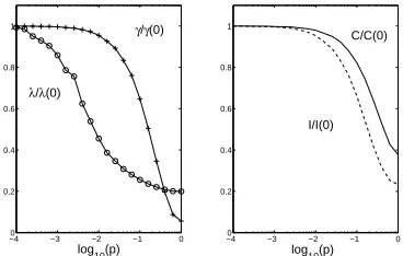
Fig. 1. How complexity, integration, path length and clustering vary as a one-dimensional ring lattice is gradually eroded by random rewiring. The ring comprises

N = 256 nodes connected to their k = 10 nearest neighbours. The left-hand panel

shows the scaled characteristic path length, λ/λ(0) and the scaled clustering

coeffi-cient,γ/γ(0), versus the log of the probability of rewiring, log₁₀(p) (circles and crosses,

respectively). The right-hand panel shows the scaled complexity,C/C(0), and scaled

integration, I/I(0), versus the log of the probability of rewiring, log₁₀(p) (solid and

dashed lines respectively). Whereλ(0), γ(0), I(0) andC(0) are measures taken on a

ring lattice withp= 0.

simulating a weakly coupled system. However, this route in computationally de-manding for large ensembles of networks. Instead, here, we employ a method that allows us to an analytically calculateCOVdirectly from the adjacency matrix of a linear, connected (i.e., no disconnected sub-graphs) network [9].1

Lastly, for large networks, calculating mutual information measures over all subset sizes is also computationally demanding. Here, unless otherwise stated, we calculate the complexity as an average over subset sizes i ≤ 4. This was observed to give a good approximation of full complexity for all models.

In addition to measuring behavioural complexity, we make use of two stan-dard graph theoretic measures: clustering and characteristic path length. The nodal clustering coefficient is defined as the number of connections between the neighbours of a given node divided by the total number of possible connections between them [4]. The graph clustering coefficient,γ, (simply referred to as the clustering coefficient form henceforth) is calculated as the mean nodal cluster-ing coefficient over a network’s nodes. A network’s characteristic path length,λ, is the average length of the shortest paths connecting all pairs of nodes [4]. In contrast to the clustering coefficient this is a global property of the graph.

All results reported here are averaged over no less than 30 networks per data point, and standard deviations were consistently lower than 0.5%.

1 _{For the matlab code for this and many of the other calculations employed in this}

Small-worlds Intuitively, the small-world effect, where systems combine strong clustering with short characteristic path lengths, would seem commensurate with high complexity. Clustering suggests functional segregation, while a sparse web of longer-range connections could encourage functional integration at a global level. Furthermore, the small-world property and high complexity have been shown to be coincident in biological neural systems [7].

Initially, we replicate the original small-world experiment presented in [4]. Commencing with a one-dimensional ring comprisingN = 256 nodes, each con-nected to their k = 10 nearest neighbours, and representing these interactions as a binary connection matrix, each connection (edge) has probabilitypof being randomly rewired to another node while preserving the in degree at each node. Note: unlike Watts we use directed graphs. For a range of rewiring probabilities, we calculate the resulting values of γ,λ, and also calculate the complexity, C, and integration,I, as outlined in section 2.

Fig. 1 presents these measurements scaled by the values associated with the original ring lattice, see caption for further details. While a low probability of rewiring generates a small-world effect in reducing characteristic path length without damaging clustering, both complexity and integration fall monotonically withp(as mentioned recently in [7]). Essentially, the spatial organisation of the lattice is being eroded by rewiring. However, perhaps this result is specific to a rewired lattice which only exhibits a single topological scale of organisation. Note: while clustering coefficient seems to refer to an intuitive idea of distinct clusters in fact this is not the case and even a lattice has a high clustering coefficient. Instead consider Watts’ connected cave world [10], for example, which exhibits two topological scales, that of the tightly intra-connected local clusters (caves), and a global level of loose inter-cluster connections. To explore this we examine four different structures: a one-dimensional ring is presented for comparison with fig. 1; a toroidal structure represents extending such a ring into a second spatial dimension; a “connected cave-world” [4] consists of a set of 32 fully-connected caves of 8 nodes each arranged on a ring with 8 connections between each pair of caves, representing a simple clustered network; a fractal structure similar to those employed in [7]. To build this fractal structure we start with a fully-connected clique of 8 nodes, duplicate it, and connect nodes from one cluster with nodes in the other according to some connection probability. The resulting structure is again duplicated and connections between the new pair are added. This process repeats until there are 256 nodes. Note: the probability of inter-cluster connections is reduced exponentially over fractal levels (see [7]).

probabil-−40 −3 −2 −1 0 5

10 15 20

log₁₀(p)

Small−world Index (S)

log₁₀(p)

−40 −3 −2 −1 0

0.5 1 1.5 2 2.5 3 3.5 4 4.5 5

Complexity (C/C(p=1))

1D

Connected Cave−world

2D

Fractal

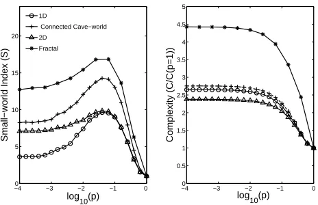
Fig. 2. The left-hand panel shows how the small-world index, S = γ/γ_λ/λ(₍p_p=1)₌₁₎, varies with the log of the probability of rewiring, log10(p), for four network structures. The

right-hand panel shows how the scaled complexity, C/C(p = 1), varies for the same

network structures. All networks comprise N = 256 nodes with identical connection

densities (N/K ≈ 0.03). (The different network structures necessitate that different

degree distributions must be compared.) Here C(p = 1) is the value of complexity

associated with a random graph (i.e., when the probability of rewiring is unity).

ity of rewiring. By contrast, the consonant variation in characteristic path length appears to have little or no influence.

Spatial Length Scales The impact of spatial embedding is not limited to its effect on clustering coefficients and characteristic path lengths. Rather, (at minimum) it is capable of bringing about structural organisation over a partic-ular length scale. Here, we explore ensembles of spatially constrained networks constructed over nodes distributed uniformly in hypercubes of varied dimen-sionality, varying the length scale of the interaction between the nodes. Note: in order to preserve the magnitude of spatial relationships between pairs of nodes over different numbers of dimensions all distances are scaled by 1/√d. In-stead of the binary connection matrixes used above, here we employ continuous-valued entries to represent weighted connections between pairs of nodes given by

ωij =exp(−|rj−ri|/σ). Where,|rj−ri|is the distance between nodesiandj. Connection weights between pairs of nodes fall exponentially with distance at a rate which is defined by the interaction length,σ. Fig. 3 shows how complexity,

C, varies with the log of the interaction strength, log10(σ).

−3.50 −3 −2.5 −2 −1.5 −1 −0.5 0 0.02

0.04 0.06 0.08

Complexity (C)

Complexity (C)

−3.50 −3 −2.5 −2 −1.5 −1 −0.5 0 0.02

0.04 0.06 0.08

−3.50 −3 −2.5 −2 −1.5 −1 −0.5 0 0.02

0.04 0.06 0.08

log

10 (σ) log10 (σ)

−3.50 −3 −2.5 −2 −1.5 −1 −0.5 0 0.02

0.04 0.06 0.08

1D 2D

128D 3D

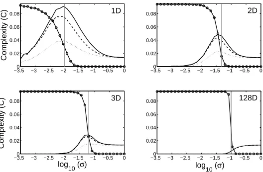
Fig. 3. Plots of complexity C versus the log of the interaction length, log10(σ) ,for

1, 2, 3, and 128 dimensions are presented in the top left, top right, bottom left and

bottom right panels, respectively.All networks comprise N = 128 nodes. The solid

curves represent the mean complexity,C, of spatially embedded system with continuous

weights. The dotted and dashed lines indicates the complexity of networks derived from two null models (see text). The grey vertical lines mark the peaks of complexity for discretised networks with the same interaction length, which agree well with the peak in complexity for the associated continuous system (the solid line). The scaled number of

network components is also presented (circles), falling fromN (a totally disconnected

system) to unity (a super cluster).

be drawn and their properties calculated. For each network, we enumerate the number of disconnected components. As this value approaches unity, the graph is becoming completely connected, indicating the onset of a single component or super-cluster [10].

For comparison, all plots in fig. 3 also present values of complexity for two null models. First, the dotted line represents the complexity of networks where each node has the same distribution of afferent connection strengths, but the identity of neighbours is randomly assigned. To achieve this, the entries of each row in the weight matrix are shuffled, preserving the sum of afferent weights. The dashed line represents the complexity of networks for which connections are shuffled in a way that preserves reciprocity, i.e., where a shuffle swaps elements

−2.6 −2.4 −2.2 −2 −1.8 −1.6 −1.4 −1.2 0.015

0.02 0.025 0.03 0.035 0.04

0.045 Inter and Intra

Niether Inter nor Intra Intra only Inter only Completely randomised

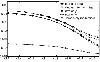
Fig. 4. Complexity, C, varies with cluster width for networks with spatial structure within and/or between each of 12 regularly arranged clusters of nodes distributed in

two-dimensional space according to a normal distribution with variance, σspace. The

complexity of equivalent non-spatial random networks is shown for comparison.

The first point to note is that for low-dimensional spaces, complexity rises and falls with interaction length.2

As the dimensionality of the space increases, peak complexity falls. The reciprocal nature of spatial interactions clearly ac-counts for this effect to some extent (and to a larger degree than the mere distribution of afferent weights). However, particularly in low dimensions, the impact of spatial constraints exceeds that of mere reciprocity, suggesting that higher-order structures are significant. As the dimensionality of the space in-creases, and the strength of spatial constraints weaken, peak complexity falls, until the contribution of space, and even reciprocity disappears.

Interestingly, the peak in network complexity is correlated with the onset of the super cluster in the discretised versions of the networks presented in fig. 3. Although the graph theoretic measure does not directly translate into the continuous domain, this result suggests that complexity is associated with the achievement of a single strongly coupled component in a continuous network. Furthermore the interaction length required for onset of the strong component (and thus high complexity) falls with the dimensional order.

Spatial Structure Thus far, we have only considered uniform spatial dis-tributions of points. However, spatio-temporal processes naturally bring about structured distributions. Here we consider how the introduction of community structure, in the form of randomly distributed clusters of equal size, impacts on network complexity. In contrast to clustering coefficient community structure provide a more intuitive notion of clustering [11].

Here N = 126 nodes are divided into 9 groups of 14 points. The group foci are regularly arranged as a 3×3 grid in the unit square. The points of

2 _{Since the covariance matrix of a 1-d lattice is of Gaussian Toeplitz form, this agrees}

each group are then normally distributed around each focus with a variance

σspace(note: this is distinct from the interaction length,σ). For increasingσspace, distinct, tight clusters (communities) initially spread, then merge, and eventually overlap to form a virtually uniform distribution of nodes. The connection weight between each pair of nodes is determined as per the previous model with a fixed interaction lengthσ= 10−3.

We wish to distinguish the contribution to complexity made by within-cluster spatial correlation structure from that contributed by between-cluster organi-sation. We achieve this by selectively extinguishing the spatial correlations at each scale, either shuffling the afferent weights of each node’s intra-cluster con-nections, or each node’s inter-cluster concon-nections, or both. All three shuffling processes preserve the degree density within each cluster and between each pair of clusters. Lastly, by shuffling every row of the weight matrix, we generate fully randomised networks for which only the distribution of weight strengths is preserved.

Fig. 4 shows that as the cluster width increases and clusters merge, com-plexity falls, suggesting that non-uniform spatial distributions impact on net-work complexity. Here netnet-work complexity can be partitioned into contributions due to inter-cluster spatial constraints, intra-cluster spatial constraints, and the residual community structure arising from the fact that, to the extent that clus-ters are spatially distinct from one another, there will tend to be stronger weights on within-cluster connections than between-cluster connections. The latter con-tribution dominates until cluster widths approach the width of the space, result-ing in an approximately uniform distribution. By contrast, the contribution of within-cluster spatial organisation is minimal until nodes approximate a uniform distribution. Inter-cluster spatial constraints make a consistent but relatively small contribution to complexity across the range of cluster widths.3

4

Discussion & Conclusion

First, by systematically exploring the relationship between the small-world effect on a networks topology and the consequent behavioural complexity that the network exhibits, we have shown that although these two properties may co-occur in natural systems [7], it is not the case that small-world structures alone straightforwardly imply complex network behaviour (see figs. 1 and 2).

However, as intimated in recent work [7], results here demonstrate that spa-tial constraints on connectivity contribute directly to complexity. Even in the absence of the community structure or fractal organisation that is known to generate complex network behaviour [7], networks merely comprising uniform random distributions of locally connected nodes enjoy increased complexity as a result of the strong spatial constraints imposed by low dimensionality (see fig. 3). The nature of the contribution to complexity made by spatial embedding is not straightforward. Neither the shape of the distribution of afferent weights

3 _{These results are redolent of the differences in complexity between ordered and}

(dotted lines, fig. 3) nor their reciprocity (dashed lines, fig. 3) are sufficient to account its impact on complexity. Rather, the property stems from space impos-ing correlations at several topological scales. This is evidenced by the gradual erosion of the influence of space as dimensionality is increased (see fig. 3).

Fig. 3 suggests that high network complexity is correlated with the onset of strongly coupled super cluster. The coupling strength required for its onset is much smaller in networks embedded within low-dimensional spaces suggest-ing that strong spatial constraints may make high complexity easier to achieve despite sparse or weak connections.

Finally, we have shown that the structure of the underlying spatial distri-bution of nodes can impact on network complexity. For example, results sug-gest that clusters of nodes randomly distributed in space bring about network topologies that exhibit high complexity stemming from both inter-cluster and intra-cluster correlations, but mostly by the residual community structure that distinct clusters impose (perhaps justifying the current focus on hierarchical and fractal organisation with respect to neural systems [6, 5]).

In summary, as suggested by the evolvability of some spatially embedded network architectures [12], the inherent constraints imposed by projecting sys-tems into low dimensional spaces may be enabling for evolution in that they predispose systems to exhibit complex behaviour for free.

AcknowledgementsWe thank Olaf Sporns for his email discussions.

References

1. Langton, C.G.: Computation at the edge of chaos. Physica D42(1990) 12 – 37

2. Kauffman, S.: The Origins of Order. Oxford University Press, Oxford (1993) 3. Boerlijst, M.C., Hogeweg, P.: Spiral wave structure in pre-biotic evolution:

Hyper-cycles stable against parasites. PhysicaD 48(1991) 17–28

4. Watts, D.J., Strogatz, S.H.: Collective dynamics of ’small-world’ networks. Nature

393(1998) 440–442

5. Tononi, G., Sporns, O., Edelman, G.M.: A measure for brain complexity: Relating functional segregation and integration in the nervous system. Proc Natl Acad Sci

91(1994) 5033–5037

6. Sporns, O., Tononi, G., Edelman, G.M.: Theoretical neuroanatomy: Relating

anatomical and functional connectivity in graphs and cortical connection matrices.

Cerebral Cortex10(2000) 127–141

7. Sporns, O.: Small-world connectivity, motif composition, and complexity of fractal

neuronal connections. Biosystems85(2006) 55–64

8. Hoppensteadt, F.C., Izhikevich, E.: Weakly Connected Neural Networks. Springer-Verlag, New-York (1997)

9. Tononi, G., Edelman, G.M., Sporns, O.: Complexity and coherency: integrating

information in the brain. Trends in Cognitive Sciences2(1998) 474–483

10. Watts, D.J.: Small Worlds. Princeton University Press, Princeton (1999)

11. Girvan, M., Newman, M.E.J.: Community structure in social and biological

net-works. Proc Natl Acad Sci99(2002) 7821–7826

12. P. Husbands, T. Smith, N.J., O’Shea, M.: Better living through chemistry: Evolving