This is a repository copy of
Multivariate Topology Simplification
.
White Rose Research Online URL for this paper:
http://eprints.whiterose.ac.uk/100068/
Version: Accepted Version
Article:
Chattopadhyay, A, Carr, H, Duke, D et al. (2 more authors) (2016) Multivariate Topology
Simplification. Computational Geometry, 58. pp. 1-24. ISSN 0925-7721
https://doi.org/10.1016/j.comgeo.2016.05.006
© 2016, Elsevier. Licensed under the Creative Commons
Attribution-NonCommercial-NoDerivatives 4.0 International
http://creativecommons.org/licenses/by-nc-nd/4.0/
Reuse
Items deposited in White Rose Research Online are protected by copyright, with all rights reserved unless indicated otherwise. They may be downloaded and/or printed for private study, or other acts as permitted by national copyright laws. The publisher or other rights holders may allow further reproduction and re-use of the full text version. This is indicated by the licence information on the White Rose Research Online record for the item.
Takedown
If you consider content in White Rose Research Online to be in breach of UK law, please notify us by
Multivariate Topology Simplification
Amit Chattopadhyaya,b,1, Hamish Carra,2, David Dukea,3, Zhao Genga,4, Osamu Saekic,5
aSchool of Computing, University of Leeds, LS2 9JT, Leeds, UK. bInternational Institute of Information Technology, Bangalore, India.
cInstitute of Mathematics for Industry, Kyushu University, Motooka 744, Nishi-ku, Fukuoka 819-0395, Japan.
Abstract
Topological simplification of scalar and vector fields is well-established as an effective method for analysing and visualising complex data sets. For multivariate (alternatively, multi-field) data, topological analysis requires simultaneous advances both mathematically and computationally. We propose a robust multivariate topology simplification method based on “lip”-pruning from the Reeb space. Mathematically, we show that the projection of the Jacobi set of multivariate data into the Reeb space produces a Jacobi structure that separates the Reeb space into simple components. We also show that the dual graph of these components gives rise to a Reeb skeleton that has properties similar to the scalar contour tree and Reeb graph, for topologically simple domains. We then introduce a range measure to give a scaling-invariant total ordering of the components or features that can be used for simplification. Computationally, we show how to compute Jacobi structure, Reeb skeleton, range and geometric measures in the Joint Contour Net (an approximation of the Reeb space) and that these can be used for visualisation similar to the contour tree or Reeb graph.
Keywords: Computational Topology, Simplification, Multivariate, Reeb Space, Reeb Skeleton, Joint Contour Net, Multi-Dimensional Reeb Graph.
1. Introduction
Scientific data is often complex in nature and difficult to visualise. As a result, analytic tools have become increasingly prominent in scientific visualisation, and in particular topological analysis. While earlier work dealt primarily with scalar data [1,2,3], multivariate topological analysis in the form of the Reeb space [4,5] has started to become feasible using a quantised approximation called the Joint Contour Net (JCN) [6].
Prior experience in scalar and vector topology shows that simplification of topological struc-tures is required, as real data sets are often noisy and complex. Although most of the work required is practical and algorithmic in nature, mathematical formalisms are also needed, in this
1Corresponding Author. e.mail address: [email protected] 2e.mail address: [email protected]
3e.mail address: [email protected] 4e.mail address: [email protected] 5e.mail address: [email protected]
case based on fiber analysis, in the same way that Reeb graphs and contour trees rely on Morse theory. This paper therefore:
1. Clarifies relationships between the Reeb space of a multivariate map f, the Jacobi set of f, and fiber topology,
2. Introduces the Jacobi structurein the Reeb space that decomposes the Reeb space into regularandsingularcomponents equivalent to edges and vertices in the Reeb graph, then reduces it further to aReeb skeleton,
3. Proves that Reeb spaces for topologically simple domains have simple structures with properties analogous to properties of the contour tree, allowinglip-pruningbased simpli-fication,
4. Introduces therange measureand other geometric measures for a total ordering of regular components of the Reeb space,
5. Describes an algorithm that extracts the Jacobi structure from the Joint Contour Net using aMulti-Dimensional Reeb Graph(MDRG) and computes the Reeb skeleton, and
6. Simplifies the Reeb skeleton and the corresponding Reeb space computing the range and other geometric measures using the JCN.
To clarify the relationships between the newly introduced data-structures in the current paper, note that the JCN is an approximation of the Reeb space. We compute a MDRG from the JCN. The critical nodes of the MDRG form the Jacobi structure of the JCN. The Jacobi structure then separates the JCN into regular and singular components. The dual graph of such components gives a Reeb skeleton which is used in the multivariate topology simplification.
As a result, much of this paper addresses the theoretical machinery for simplification of the Reeb space and its approximation, the Joint Contour Net. Section2reviews relevant background material on simplification, followed by a more detailed review of the fiber topology, Jacobi set and Reeb space in Section3. Section4provides theoretical analysis and results needed for the lip-simplification of the Reeb space. For simple domains, the Reeb space can have detachable (lip) components: this is used in Section5 to generalise leaf-pruning simplification from the contour tree to the Reeb space. Once this has been done, we introduce a range persistence and other geometric measures to govern the simplification process.
In Section6, we give an algorithm for simplifying the Joint Contour Net. We start by build-ing a hierarchical structure called the Multi-Dimensional Reeb Graph that captures the Jacobi structure of the Joint Contour Net, and then show how to reduce the JCN to a Reeb skeleton - a graph with properties similar to a contour tree. In Section7, we illustrate these reductions first with analytic data where the correct solution is knowna priori, then for a real data from the nuclear physics. As part of this, we provide performance figures and other implementation details in Section7, then draw conclusions and lay out a road map for further work in Section8.
2. Previous Work
2.1. Scalar Field Simplification
The topological complexity of the scalar field data is measured in terms of the number of critical points and their connectivities - captured by its Reeb graph or contour tree. Another way to capture the topological complexity of the scalar field is by computing the Morse-Smale complex of the corresponding gradient field. Therefore, the topological simplification in this case is driven by reducing the number of critical points via simplification of the Reeb graph, contour tree or the Morse-Smale complex. Carr et al. [2] describe a method for associating local geometric measures such as the surface area and the contained volume of contours with the contour tree and then simplifying the contour tree by suppressing the minortopological features of the data. Note that a feature is any prominent or distinctive part or quality that characterises the data and topological features captures the topological phenomena of the underlying data. Wood et al. [7] give a Reeb graph based simplification strategy for removing the excess topology created by unwanted handles in an isosurface using a measure for computing the handle-size in the isosurface and associating them with the loops of the Reeb graph. Gyulassy et al. [8] describe a technique for simplifying a three-dimensional scalar field by repeatedly removing pair of critical points from the Morse-Smale complex of its gradient field, by repeated application of a critical-point simplification operation. Mathematically, the simplification of “lips” proposed in this paper is a direct generalization of this idea (for scalar fields) to multi-fields. Luo et al [9] describe a method for computing and simplifying gradients and critical points of a function from a point cloud. Tierny et al. [3] present a combinatorial algorithm for simplifying the topology of a scalar field on a surface by approximating with a simpler scalar field having a subset of critical points of the given field, while guaranteeing a small error distance between the fields.
The topological complexity of a point cloud data can be measured by its homology. For a point cloud data inR3 this is expressed by the topological invariants, such as the Betti num-bers corresponding to a simplicial complex of the point cloud - denoted byβ0(number of con-nected components),β1 (number of tunnels or 1-dimensional holes) andβ2 (number of voids or 2-dimensional holes). Thei-th Betti number represents the rank of thei-th homology group (i=0,1,2). Edelsbrunner et al. [10] introduce the idea of persistence for the topological simplifi-cation of a point cloud by reducing the Betti numbers using a filtration technique. Cohen-Steiner et al. [11] extend the persistence diagram for scalar functions on topological spaces and analyze its stability.
In addition, several methods have been recently introduced for the comparison of Reeb graphs including the combinatorial edit distance [12], the interleaving distance [13], and the functional distortion distance [14]. However, none of these has been fully investigated for the Reeb space.
2.2. Mesh Simplification
Mesh-simplification is well-known in the computational geometry and graphics community. Topological complexity of a mesh can be determined by its genus. Guskov et al. [15] remove the unnecessary topological noise from meshes of laser scanner data by reducing their genera. Nooruddin et al. [16] give a voxel-based simplification and repair method of polygonal models using a volumetric morphological operation. Ni et al. [17] generate a fair Morse function for ex-tracting the topological structure of a surface mesh by user-controlled number and configuration of critical points. Hoppe et al. [18] describe a energy-minimization technique for generating an optimal mesh by reducing the number of vertices from a given mesh. Also Hoppe et al. [19,20] give a new progressive mesh representation, a new scheme for storing and transmitting arbitrary triangle meshes, and their simplification technique. Chiang et al. [1] describe a technique of
progressive simplification of tetrahedral meshes preserving isosurface topologies. Their method works in two stages - first they segment the volume data into topological-equivalence regions and in the second step they simplify each topological-equivalence region independently by edge collapsing, preserving the iso-surface topologies. There are many cost-driven methods of mesh-simplification (in the literature) which attempt to measure only the cost of each individual edge collapse and the entire simplification process is considered as a sequence of steps of increasing cost [21,22,23,24].
2.3. Vector Field Simplification
Topology based methods for vector field simplification are based on the idea ofsingularity pair cancellationto reduce the number of singularities and thus the topological complexity. This method iteratively eliminates suitable pairs of singularities with opposite Poincar´e-Hopf indices so that total sum of the indices remain invariant to keep the global structure of the field the same. This idea has been exploited in [25,26,27]. There are also non-topology based methods for vector-field simplification which are mainly based on smoothing operations. Smoothing oper-ations reduce vector and tensor-field complexity and remove large percentage of singularities. Polthier et al. [28] apply Laplacian smoothing on the potential of a vector-field. Tong et al. [29] decompose a vector field into three components: curl free, divergence free and harmonic. Each component is smoothed individually and results are summed to obtain simplified vector field.
2.4. Multi-Field Simplification
To the best of our knowledge, until now there is no prior work on topology-based simpli-fication of general multi-field data. All those techniques, cited so far, for simplifying scalar fields, meshes and vector fields are not directly applicable in case of multi-fields, primarily be-cause the computation of the equivalent tools such as, Jacobi set [30], Reeb space [5] are not well-developed. A generalization of the persistent homology is proven to be difficult for the multi-fields [31].
Singh et al. [32] introduced the idea ofmapperthat is based on a partial clustering of high-dimensional data guided by the fields defined on the data. A mapper extracts the nerve of a covering defined by the clusters. Conceptually, the recently introducedJoint Contour Net[6] is a particular case of mapper construction, namely the nerve of a particular choice of cover for
Rr that will be discussed in section6.1. However, the main idea of mapper was moving from topological to a statiscal version using the notion of clustering, whereas the joint contour net uses the notion of joint contour slabs and their topological connectivity. In the current paper we use joint contour net as a tool for further simplification of multivariate data.
Few attempts have been made for simplifying the Jacobi sets in restrictive cases. Snyder [33] gives two metrics for measuring persistence of the Jacobi sets. Bremer et al. [34] describe a method for noise removal from the Jacobi sets of time varying data. Suthambhara et al. [35] give a technique for the Jacobi set simplification of bivariate fields based on simplification of the Reeb graphs of their comparison measures. Huettenberger et al. propose multi-field simplification method using Pareto sets [36,37]. However, these methods lack mathematical justification for simplifying the corresponding input multi-fields and work mostly for bivariate data. In a similar context, Bhatia et al. [38] provide a simplification method by generalising the critical point cancellation of scalar functions to the Jacobi sets in two dimensional domains.
Recently, Multi-Dimensional Reeb Graphs [39] and Layered Reeb Graphs [40] have been intro-duced from two different perspectives to extend the Reeb graph for multi-fields. In the current paper, we use the recently introduced Jacobi structure [39] to separate the Reeb space into regular and singular components. Thus we obtain a dual Reeb skeleton corresponding to the Reeb space. Our simplification strategy is based on simplifying this Reeb skeleton by associating different measures with the nodes of the Reeb skeleton.
3. Necessary Background
[image:6.595.191.403.343.479.2]Over the last two decades, scalar topology has been used to support scientific data analysis and visualization, in particular through the use of the Reeb graph and its specialisation, the contour tree [41,42,43,44,45]. The subject of multi-field topology in data analysis is rather new. In this section we briefly describe the multi-field topological analysis and existing tools for capturing them, viz. the Jacobi set and the Reeb space.
Table 1: Important Notations
Notation Name
Wf Reeb space
Kf Reeb skeleton
Jf Jacobi set
J∂
f Boundary Jacobi set
J◦f Interior Jacobi set Jf Jacobi structure
JCN(f;M,mQ) Joint Contour Net w.r.t. meshM and quantization levelmQ
Rf
i Reeb graph
Mf Multi-dimensional Reeb Graph
3.1. Multi-Field Analysis
A multi-field on a d-manifold X(⊆Rd)with r component scalar fields fi:X→R(i= 1, . . . ,r) is amap f = (f1, f2, . . . , fr):X→Rr. Table1 shows the notations used to denote various structures corresponding to a multi-field f in the current paper.
In differential topology, f is considered to be asmooth mapwhen all its partial derivatives of any order are continuous. A pointx∈Xis called asingular point(orcritical point) of f if the rank of its differential mapd fxis strictly less than min{d,r}whered fxis ther×dmatrix whose rows are the gradients of f1to fratx. And the corresponding value f(x) =c= (c1,c2, . . . ,cr) inRris asingular value. Otherwise if the rank of the differential mapd f
xis min{d,r}thenxis called aregular pointand a pointy∈Rris aregular valueif f−1(y)does not contain a singular point.
The inverse image of the map f corresponding to a valuec∈Rr, f−1(c)is called afiber and each connected component of the fiber is called afiber-component[46,4]. In particular, for a scalar field these are known as thelevel setand thecontour, respectively. The inverse image of a singular value is called asingular fiberand the inverse image of a regular value is called a
(a) A B C D E 1 2 3 4 5 6 7 8 9 (b) 1 2 3 4 5 6 7 8 9 (c) f1 f2 (d) A B C D E
BCDE
1' 2',3',4',5'
6' 7'8'9'
(e) 2' 1' 3' 4' 9' 5',6',7',8' (f)
Figure 1: (a) A stable bivariate field(f1,f2)≡(x2+y2+z2,z)fromR3toR2that is visualized using the transparent
isosurfaces of the first component field; black curves are the fiber-components of the bivariate field; the red line represents the Jacobi set; (d) The Reeb space corresponding to (a) that is comprising one sheet (in pink) and the Jacobi structure (red parabolic curve); (b) The Jacobi set (consists of the red lines, top face and bottom face of the box) of the bivariate field
(f1,f2)≡(x2+y2,z)in the box[−1,1]×[−1,1]×[0,1]; singular fibers passing through the boundary tangent points
form a cylindrical surface that separates the domain into five components, denoted as A, B, C, D and E; (e) The Reeb space of the multi-field corresponding to (b) that is comprising five sheets (in grey) and the Jacobi structure (red lines); the regular components of the Reeb space are marked to match the corresponding components in the domain; components of the Jacobi set in the domain and their corresponding projections in the Reeb space are denoted by numbers; (c) An unstable bivariate field(f1,f2)≡(x4+y4+z4−5(x2+y2+z2) +10,z)fromR3 toR2 that is visualized using the
transparent isosurfaces of the first component field; black curves are the fiber-components of the bivariate field; the Jacobi set consists of 9 red lines; (f) The Reeb space corresponding to (c) that is comprising six sheets and the Jacobi structure (6 red lines).
regular fiber. If a fiber-component passes through a singular point, it is called asingular fiber-component. Otherwise, it is known as aregular fiber-component. Note that a singular fiber may contain a regular fiber-component.
[image:7.595.113.488.151.485.2]and it is said to bestableif its topological properties remain unchanged by small perturbations [47]. Let f :X⊂R3→R2be a proper smooth map. Then, it is stable if and only if it satisfies the following local and global conditions. Around each singular points, f is locally described as either (i)(u,x2+y2):sis a definite fold point, or (ii)(u,x2−y2):sis an indefinite fold point, or (iii)(u,y2+ux−x3/3):sis a cusp point, for some local coordinates(u,x,y)aroundsand an appropriate set of local coordinates around f(s)in the rangeR2. Moreover, no cusp point is a double point of f restricted to the set of singular points and f restricted to the set of all definite and indefinite fold points is an immersion with normal crossings. Thus for a proper stable map, a singular fiber-component passing through a definite fold point or a cusp point contains exactly one such point, while a singular fiber-component passing through an indefinite fold point may pass through one or two indefinite fold points. Otherwise, the map is called anunstable map.
We note, characterizing the stability of the maps on compact 3-manifold domains with bound-ary needs additional types of singularities which is discussed in [48]. Figure1ais an example of a map fromR3toR2where f= (x2+y2+z2,z). All its singular points are definite fold points, so this is an example of a stable map. Figure1cis an example of a map fromR3toR2where f= (x4+y4+z4−5(x2+y2+z2) +10,z). It has singular fiber-components which pass through four indefinite fold points (on corresponding four 1-manifold components numbered as 5, 6, 7 and 8 in Figure1c) and so is an example of an unstable map.
From the pre-image theorem [49], generically a regular fiberf−1(c)is a(d−r)-manifold for the regular valuec= (c1,c2, . . . ,cr). We note ford<r,f−1(c)is an empty set or a discrete set of points. A fiberf−1(c)can be considered as the intersection of the fibers of the component scalar fields f1−1(c1),f2−1(c2), . . . , fr−1(cr)and a connected component of this intersection is a fiber-component. Alternatively, fiber-components of(f1, f2, . . . , fr)can be considered as the contours of a component field fi, restricted to the fiber-components of the remaining component fields. This is akey observation, we use in building our Multi-Dimensional Reeb Graph data-structure.
3.2. Jacobi Set
The compactd-manifold domainX(⊆Rd)of the map f can be expressed asX=X◦∪∂X
whereX◦ denotes the interior (the set of interior points) of the domain and ∂X denotes the boundary (the set of boundary points) ofX. In case the domainXis without boundary,∂X=/0
andX=X◦.
Now theinterior Jacobi setof the map f :X→Rr is denoted byJ◦
f and is defined by the setJ◦
f:={x∈X◦| rankd fx◦<min{d,r}}[50] where f◦is the restriction of f toX◦, i.e., f◦:= f|X◦:X◦→Rr. In other words,J◦f is the set of singular points of the mapfinterior to the domain
X. Similarly, theboundary Jacobi setof the map f is denoted byJ∂
f and is defined as the set of singular points of the restriction of f to the boundary∂X, i.e. f∂:=f|∂X:∂X→Rr. Finally, by
theJacobi setof the map f :X→Rrwe mean the union of the interior and the boundary Jacobi set of the map f, and is denoted byJf, i.e.Jf =J◦
f∪J∂f.
Now the boundary of a domain may come with corners, e.g. a 3-dimensional cube has corners of two types: 12 edge corners, and 8 vertex corners (as in Figure1b). Let X be a
compact 3-dimensional manifold with corners andf :X→R2be a smooth map. A pointq∈∂X is a (boundary) regular point if f restricted to∂Xis a local homeomorphism aroundq, where
∂Xstands for the boundary of X which includes all the boundary points and corner points. Otherwise,qis a (boundary) singular point. For example, if we take a point in a vertical edge in Figure1b, then in its (2-dimensional) neighborhood on the boundary, there are always a pair of
points that are mapped to the same point. Thus, it is never injective, and hence is never a local homeomorphism. Therefore, the point is a (boundary) singular point.
Alternatively, the Jacobi set is the set of critical points of one component field (say fi) of f restricted to the intersection of the level sets of the remaining component fields. Edelsbrunner et al. [50] studied properties of the Jacobi set forrMorse functions. They proved the Jacobi set is symmetric with respect to its component fields. They also showed, generically, the Jacobi set of two Morse functions is a smoothly embedded 1-manifold where the gradients of the functions become parallel. However, in general Jacobi sets are not sub-manifolds of the domain of the multi-field f, and are the disjoint union of sub-manifolds of the domain [50]. The red lines in Figures1aand1cillustrate the Jacobi sets of multi-fields on domains without boundary.
3.3. Reeb Space
As with the Reeb graph of a scalar field, the Reeb space parametrizes the fiber-components of a multi-field and its topology is described by the standard quotient space topology. We note the fiber-components of a continuous map f:X→Rr(X⊆Rd) partition the domainXinto a set of equivalence classes, denoted byWf :=X/∼, where two pointsa,b∈Xare equivalent ora∼b if f(a) =f(b)anda,bbelong to the same fiber-component of f−1(f(a))and f−1(f(b)). Now the canonical projection mapqf:X→X/∼that maps each element ofXto its equivalence class defines the standard quotient topology where open sets are defined to be those sets of equivalence classes with an open pre-image, under mapqf. The Reeb space of f is the quotient spaceWf together with this quotient topology. The decomposition of f as the composition ofqf and ¯f, where ¯f :Wf →Rr is such that f = f¯◦q
f. This is called the Stein factorisation of f. The following commutative diagram describes this relationship between the maps.
X Rr
Wf
qf
f
¯ f
Now to construct a fiber f−1(a), instead of going directly fromRr toXone can compute the pre-image under ¯f ofa. Each fiber consists of a number of components, one for each point in
¯
f−1(a). Generically, the Reeb space is a Hausdorff space, i.e., any two distinct points ofWf have disjoint neighbourhoods. Moreover, whenr≤dthe Reeb space corresponding to the multi-field
f consists of a collection ofr-manifolds glued together in complicated ways [5].
4. Theoretical Results
In this section we exploit the underlying structure of the Reeb space to decompose it into a set of simple manifold-like components (namely regular and singular components) and capture their connectivities by a dual skeleton graph (namely Reeb skeleton). Then, since in real applications most of the data come with simple domains (such as, a cube or a box), we study properties of the Reeb space and its representative skeleton graph for such topologically simple data-domains. More precisely, to prove our theoretical results in this section we consider a stable bivariate field f= (f1,f2):X→R2whereX(⊆R3)is a three-dimensional bounded, closed interval. However, most of the results are straight-forward to generalize for multi-fields of higher dimensions. Thus the domainX, we consider, is a compact domain with boundary and is simply-connected and in this case the Reeb space is path-connected.
4.1. Path Connectedness
For a continuous map f :X⊆R3→R2the Reeb space is the quotient space of its fiber-components. Note that the Reeb space is path-connected (or 0-connected), i.e., any two points p0andp1of the Reeb space can be connected by a pathγ:[0,1]→Wf so thatγ(0) =p0and
γ(1) =p1. In other words, we say 0-connectivity is preserved by the quotient mapqf :X→Wf. This can also be stated by saying that 0-th homotopy group of the Reeb spaceπ0(Wf)remains trivial. Next we prove the following important property of the Reeb space.
Lemma 4.1. Let f :X⊆R3→R2be a continuous, generic map on a3-dimensional intervalX
andWf be the corresponding Reeb space. Let P be a continuous path between any two points on the Reeb space. Then ifWf\P is path-connected, then so isX\q−f1(P).
Proof. Consider any two points p0,p1∈Wf\P. Since Wf\Pis path-connected, ∃a path
γ:[0,1]→Wf\P withγ(0) =p0 andγ(1) =p1. Using conditions like the genericity of f,
γ(t)lifts toX\q−f1(P), i.e., there exists a pathγeinXsuch thatqf◦γ(et) =γ(t)(using the path-liftingproperty [51]). Nowγeis a path between any point ofq−f1(p0)to any point ofq−f1(p1)in
X\q−f1(P). Therefore,X\q−f1(P)must be path-connected.
Thus Lemma4.1 implies if there exists a pathP in the Reeb space whose preimageq−f1(P)
separates the domain thenPmust also separate the Reeb space. This is a useful property in detaching unimportant components from the Reeb space.
4.2. Jacobi Structure
As noted in Section3, the Jacobi set of a function is not the same as the set of singular fibers, as each point in the Jacobi set is merely a representative of a singular fiber. Moreover, the structure of the Reeb space is actually given by a projection of the Jacobi set or the singular fibers. For example, in Figures1cand1f, the Jacobi set consists of 9 parallel lines in the domain, but they correspond to 6 1-manifold structures in the Reeb space. Note that if the input multi-field domain is with boundary, there are additional edges (corresponding to the boundary Jacobi set) needed to describe the Reeb space. We therefore introduce theJacobi structure: the manifold structure of the Reeb space corresponding to the Jacobi set in the domain.
Definition 4.1. TheJacobi structureof a Reeb spaceWf corresponding to a multi-field f :X⊆ R3→R2is denoted byJf and is defined byJf :=qf(Jf), i.e., the projection of the Jacobi set
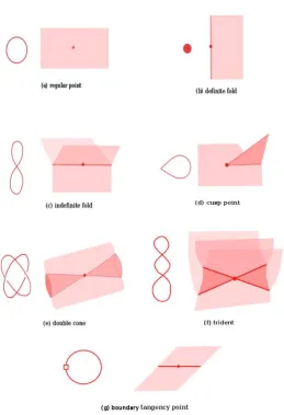
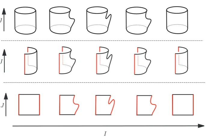
Figure 2: Regular and singular fiber-components and corresponding local configurations in the Reeb space. The Jacobi structures are in red lines in the Reeb space [48].
Note that according to our definition the Jacobi setJfconsists of both the interior and the bound-ary Jacobi set, i.e.,Jf=J◦f∪J∂f. Thus each point of the Jacobi structure corresponds to a singular fiber-component in the domainXof f, and vice-versa.
For a generic map f :X→R2,Wf is a two-dimensional polyhedron and Jacobi structure embedded in the Reeb space consists of 1-dimensional components which are at the boundary of the two-dimensional sheets inWf. Now a 1-manifold component of the Jacobi structure can be classified into three types based on the transition of number of regular fiber-components if one passes across the component [46]:
1. Birth-DeathorBoundary component- where a fiber-component is born or dies (Figure2 (b)),
2. Merge-Split componentorBifurcation locus- where two (or more) fiber-components merge together or one component splits into two (or more) (Figure2(c)) and
3. Neutral component- where there is no change in the number of fiber-components if one passes through such components (Figure2(g)), but here, the topology of the regular fiber-component changes from a circle to an arc (or vice versa).
A connected component of the Jacobi structure may also consist of a composition of these three types, e.g. in Figure2(d) the Jacobi structure component consists of a boundary and a merge-split component connected at a discretecusp point. In Figure2(e) four merge-split components are connected at adouble pointon the Jacobi structure.
Figures1band1erespectively show an example of 8 1-manifold components of the boundary Jacobi set (red lines in the boundary of the domain) and their corresponding projection in the Reeb space as 5 1-manifold parts of the Jacobi structure. From this example, it is clear that a boundary Jacobi set component may not be the boundary component of the Jacobi structure in the Reeb space or vice-versa. In Section6we propose an algorithm for computing the Jacobi structure by constructing a Multi-Dimensional Reeb Graph corresponding to a multi-field.
4.3. Regular and Singular Components
As the number of dimensions increases, the projections of the singular fibers develop more internal structure in the Reeb space. Consider the Reeb graph of a scalar function: in this, the projection images of the critical points are single points (0-manifolds) separating edges (1-manifolds). Similarly, for the bivariate fields shown in Figures1d,1eand1f, the projections of the singular fibers are arranged in a Reeb space along 1-manifold curves which separate 2-manifold sheets. This induces a natural stratification or partition of the Reeb space into disjoint subspaces (or strata).
To describe a stratification of the Reeb space and the corresponding domain of the multi-field we first classify the fiber-components of the generic map f :X⊆R3→R2according to their complexity or codimension of the subspace where they lie [46]. Given the Stein factorization
f= f¯◦qf, fiber-components of f can be classified into three classes.
1. C0={q−1
f (s):s∈Wf andq−f1(s)does not contain any singular point of f}. Fiber-components of this class are the regular fiber-components and theirqf-images form codimension 0 sub-spaces inWf, denoted asW0
f.
2. C1={q−1
f (s):s∈Wf andq− 1
f (s)contains exactly one de- finite or indefinite fold point}. Singular fiber-components of this class are moderately complex and theirqf-images form codimension 1 subspaces inWf, denoted asW1f.
3. C2={q−f1(s):s∈Wf andq−f1(s)contains a cusp point or two indefinite fold points}. Sin-gular fiber-components of this class are the most complex and theirqf-images form codi-mension 2 subspaces inWf, denoted asW2f.
Complexity of a fiber-component increases as the codimension of the corresponding subspace in the Reeb space increases. Note thatqf-images of the fiber-components inC1andC2form the Jacobi structureJf of the Reeb space, i.e., Jf =W1f∪W2f. Topologically, regular fiber-components are either a circle or an arc [48]. For stable maps f :X⊆R3→R2, topologically there are 7 different types of singular fibers inC1and 21 different types of singular fibers inC2 [48].
Two regular pointsa,b∈W0
f aretopologically equivalentin the Reeb spaceWf ora∼ρb
if there exists a path betweena andb without intersecting the Jacobi structureJf. It is not difficult to check that ‘∼ρ’ is an equivalence relation. Therefore, the equivalence relation ‘∼ρ’
partitions the regular points ofWf into a set of equivalence classes. Now we prove that each such equivalence class is a 2-dimensional sheet.
Lemma 4.2(Partition). The Jacobi structureJf of a Reeb spaceWfcorresponding to a smooth stable map f:X⊆R3→R2separates the Reeb space into a set of2-manifold components.
Proof. LetDbe a small disk in the range consisting of regular values (i.e.,Ddoes not intersect f(Jf)). Then, by Ehresmann’s fibration theorem, f restricted to f−1(D)is equivalent to the projectionD×F →D, where F is a 1-dimensional compact manifold. So, this means that qf(f−1(D))can be identified with a disjoint union of some copies ofD, where the number of copies is the same as the number of connected components ofF. Even whenDintersects with f(Jf), if we restrict f to the components of the inverse image f−1(D)that do not intersectJf,
then the same consequence holds. So, the regular sheets ofWf are locally homeomorphic toD,
and hence is a 2-manifold.
Thus we have the following definition of regular components.
Definition 4.2. A path-connected component ofWf\Jf orW0f is called a regular component.
Generically, the 0-dimensional strata are in the boundary of the 1-dimensional strata in theJf. Therefore, an equivalence relation on the set of points inW1f can be defined, similarly, where two points ofW1f are equivalent if there exists a continuous path between them without crossing the 0-dimensional strata inJf and each such equivalence class will be considered as a 1-singular component.
Definition 4.3. A path-connected component ofJf\W2forW1fis called a 1-singular component.
Note that a 1-singular component inWf may be an arc or a circle. An arc 1-singular component will also be called as anedge.
Definition 4.4. Each component ofW2
f is called a 0-singular component.
To extract a skeleton graph from the Reeb space we need adjacency of these regular and 1-singular components which are defined as follows.
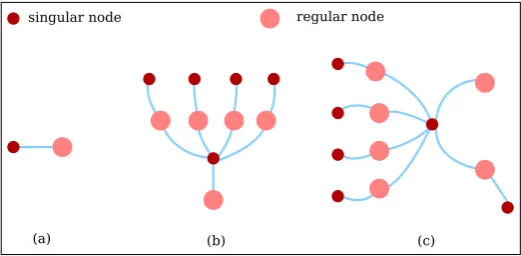
singular node regular node
[image:14.595.167.428.140.268.2](a) (b) (c)
Figure 3: Reeb skeletons: (a) corresponding to the Reeb space in Figure1d, (b) corresponding to the Reeb space in Figure1e, (c) corresponding to the Reeb space in Figure1f.
2. If two end points of an arc 1-singular component coincide, then the 1-singular component is self-adjacent.
3. Two distinct 1-singular components S1,S2are adjacent if ∃a 0-singular component α0 such that S1 ∪ S2 ∪α0form a connected space.
Definition 4.6. A 1-singular component Siis adjacent to a regular component Rjif Si∪Rjforms a connected space.
Next we define a connectivity graph of regular and singular components based on their adja-cency.
4.4. Reeb Skeleton
Once the Reeb spaceWfis split into 2-manifold regular components and 1-or-lower manifold singular components, it is possible to perform a further reduction from the Reeb space. To do so, we represent both these regular and 1-singular components as points (or nodes), and add edges representing their adjacency: in short, we can build the dual graph of these components of the Reeb space. This has the merit of further reducing the Reeb space from a 2-dimensional structure to a fundamentally 1-dimensional structure which is easier to represent, to reason about and to visualise. We refer to this as theReeb skeletonand formally define as follows.
Definition 4.7. Let R1,R2, . . . ,Rmbe the regular components and S1,S2, . . . ,Snbe the 1-singular components ofWf. Then the Reeb skeleton of f , denoted byKf, is the adjacency graph which consists of (i) nodes nRi and nSj (i=1,2, . . . ,m and j=1,2, . . . ,n) corresponding to each of
the regular and 1-singular components, and (ii) edges e(Sj,Sj′)and e(Ri,Sj)that are defined as follows:
1. If Sjis self-adjacent, then e(Sj,Sj) =1. In other words, nSj has a self-loop.
2. If Sjis self-adjacent and Sjis adjacent with a regular component Ri, then e(Ri,Sj) =2. In other words, nSj is connected with nRiby two edges.
3. If Sjand Sj′ are two distinctnon-boundary1-singular components, then
e(Sj,Sj′) =
1, if Sj,Sj′ are adjacent
Figure 4: (a) Reeb space with self-adjacent 1-singular component (b) Corresponding Reeb skeleton. The size of each node of the Reeb skeleton corresponds to the size of the corresponding Reeb space component.
4. For any regular component Riand any 1-singular component Sj
e(Ri,Sj) =
1, if Ri,Sjare adjacent 0, otherwise.
The regular and 1-singular components of the Reeb space are represented as theregularand sin-gular nodes, respectively, in the Reeb skeleton. Figure3shows some examples of Reeb skeletons corresponding to the Reeb spaces in Figure1. Figure4illustrates an example of the Reeb skele-ton with a self-adjacent singular node. Note that although the Reeb skeleskele-ton gives a simple abstraction of 0-connectivity in the Reeb space, it loses information of higher-dimensional con-nectivities, like higher dimensional holes (tunnels, voids) in the Reeb space. But on the other hand, the Reeb skeleton is extremely useful for extracting any “fork”-like structure (correspond-ing to a merge-split feature) in the Reeb space. And we will see later by a little simplification we can extract the most prominent merge-split feature in the Reeb skeleton and so in the Reeb space. Therefore, next we study properties of the Reeb skeleton to simplify it further.
4.5. Simple Domains
We know from scalar fields that topologically simple domains have a useful property: the Reeb graph is guaranteed to be a tree - i.e. the contour tree. This not only enables more efficient computation, but also provides straightforward mechanisms for feature extraction, simplification and visualisation. Ideally, in multi-fields, the Reeb space would also be contractible to a point. But we show this is not true, in general.
[image:15.595.184.410.140.231.2]Figure 5: Example of Reeb space with a tunnel.
Proposition 4.1(Simply-Connected). The Reeb space of a generic continuous map f :X⊆ R3→R2, on a simply-connected domainX, is simply-connected.
Proof. We consider any loop in the Reeb spaceWf. Then, it lifts to an arc inX. But, every fiber ofqf is connected, and therefore, it lifts to a loop. AsXis simply-connected, this lifted loop is null-homotopic. Therefore, itsqf-image is also null-homotopic from the continuity ofqf. This
means thatWf is simply-connected.
Therefore, if f is good enough (for example, triangulable or piecewise linear), then the Reeb space is simply-connected. This implies that the 1st homology of the Reeb space also vanishes (or is the trivial group), and therefore the Reeb space does not have a tunnel or 1-dimensional hole (i.e., a hole inside a circleS1, e.g. Figure5). Thus we have the following corollary.
Corollary 4.1. The Reeb space of a generic map f :X⊆R3→R2, on a simply-connected domainX, does not contain any tunnel or1-dimensional hole.
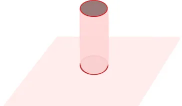
On the other hand, for void or 2-dimensional hole (i.e., hole inside a sphereS2), this is no longer true. We can construct a (piecewise linear) mapf :X→R2whose Reeb space does have a 2-dimensional hole. For example, consider the Hopf fibrationS3 → S2and its composition with a standard projectionS2 → R2. The resulting mapS3 → R2is not generic, but perturbing it slightly along its Jacobi set, we can obtain a generic mapS3 → R2, whose Reeb space is the union of a 2-sphere and an annulus attached along the equator (and one boundary component of the annulus). Then, by extracting a 3-ball in the preimage of a two disk in the interior of the annulus part, we get the desired mapX → R2. The Reeb space is the same space; the union of
S2and an annulus (Figure6). Over each blue point lies a point (definite fold) and it corresponds to a birth-death. Over each red point lies a fiber as in Figure2(c) (with an indefinite fold) and the splitting of a circle fiber occurs. Over each green point lies a circle touching the boundary of the domain cubeX. Thus, over each point in the shaded disk bounded by the green circle lies an
interval. Note this disk is a subset of the annulus part. Therefore, a Reeb space of a multi-field on a contractible domain may not be contractible and simplification of such space may not be simple as in the scalar case.
According to Theorem4.1, we can conclude that each regular component ofWf is planar; i.e., each regular component is a disk possibly with holes. For example, torus with holes (or a 1-dimensional hole as in Figure5) never appears! This is essential in applying our simplification rules for the Reeb skeleton as will be discussed in Section6.7 (Figure 12). Next we focus
xxxxxxxxxxxxxxxxxxxxxxx xxxxxxxxxxxxxxxxxxxxxxx xxxxxxxxxxxxxxxxxxxxxxx xxxxxxxxxxxxxxxxxxxxxxx xxxxxxxxxxxxxxxxxxxxxxx xxxxxxxxxxxxxxxxxxxxxxx xxxxxxxxxxxxxxxxxxxxxxx xxxxxxxxxxxxxxxxxxxxxxx xxxxxxxxxxxxxxxxxxxxxxx
Figure 6: Reeb space with a void.
on finding a criterion for detachability of such regular components from the Reeb space for simplifying the corresponding the multi-field.
4.6. Detachability
In the case of scalar field in a simply-connected domain, the Reeb space (graph) is a contour tree and there always exists a leaf edge that can be detached in a mathematically correct way, unless the contour tree consists only of one edge. We find similar criteria for definingdetachable regular components in the Reeb space.
We say that it is possible to detach a regular component from a Reeb space to obtain a sim-plified Reeb space if the multi-field corresponding to the initial Reeb space could be simsim-plified to the multi-field corresponding to the modified one, and then the regular component is said to be detachable from the Reeb space. Mathematically, any map could be simplified to a simpler map in the following sense. SinceR2is contractible, any two stable maps f
0andf1:X→R2are homotopic. So, using singularity theory, we can show that f0and f1are connected by a generic 1-parameter family of maps. So, if we take an arbitrary stable map as f0and a very simple map as f1, then f0is simplified to f1after the generic 1-parameter family. Such a 1-parameter family passes through finitely many bifurcation parameters, and such bifurcations can be classified [54]. Such transitions of the Reeb spaces for generic smooth maps on a closed 3-dimensional manifold intoR2have been studied in [54], although for maps on a 3-dimensional manifold with boundary these results need further extension. In the current paper, we consider only a simple type of singularities and show that corresponding regular component is detachable from the Reeb space. These components are known aslipsand are defined as follows.
Definition 4.8. A lip is a regular component that is attached to the other sheets of the Reeb space exactly along one edge or an arc 1-singular component, and it does not contain any vertex on the boundary, except for the two cuspidal points (Figure7(a)).
Next we prove the following lemma to show that the underlying map corresponding to a lip can be simplified.
(a) (b)
Figure 7: Lip simplification: (a) Reeb space with a lip, (b) Simplified Reeb space.
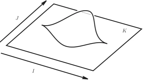
Proof. LetK be the portion of the Reeb space containing the lip in question as depicted in Figure8. We take two coordinates for describingK: one isI= [−1,1]“parallel” to the lip and the other isJ= [0,1]in the transverse direction. LetπI:K→IandπJ:K→Jdenote the natural projections, and fort∈I, setKt=πI−1(t). SinceπI◦qf :q−f1(K)→Iis a submersion, we see thatq−f1(Kt)are all diffeomorphic to a compact surface with boundary, sayS0.
Fort∈I, let ft:S0→Jbe the composition
S0=q−f1(Kt) qf
−→Kt
πJ
−→J.
In this way, we can regard the map f onq−f1(K)as a 1-parameter family of functions onS0. ForS0and ft, we have three possibilities as depicted in Figure9, whereS0 is a cylinder or a square and ft:S0→J,t∈I, is depicted as a 1-parameter family of height functions. Then, the original mapf is equivalent to the mapS0×I→J×Idefined by(x,t)7→(ft(x),t),x∈S0,t∈I, onq−f1(K)S0×I. As we can see easily, the lip corresponding to the part between the pair of critical points can be eliminated continuously, by just shrinking the “time interval” inIfor which
a pair of critical points is present.
I J
[image:18.595.184.416.492.624.2]K
Figure 8: NeighborhoodKof a lip in the Reeb space. We take two coordinates:Icorresponds to a horizontal direction “parallel” to the lip, andJcorresponds to a transverse direction.
Mathematically, “safely” here means several properties. First, the lip is eliminated by a homotopy of the original map. Furthermore, the homotopy is supported only in theqf-preimage of a small neighborhood of the lip. This means that this elimination does not change the fiber components
I J
[image:19.595.129.472.139.370.2]J J
Figure 9: The behavior of the mapqfon the pre-image of a neighborhoodKof the lip. It can be regarded as a 1-parameter
family of functionsft:S0→J,t∈I. The red lines indicate the boundary of the domain surfaceS0. For the initial time
t=−1, there are no critical points. Then astincreases, a pair of critical points appears, then their height difference increases. Att=0, the height difference starts to decrease and then the pair of critical points disappears. At the terminal timet=1, we return to the initial function.
corresponding to the rest of the Reeb space. Moreover, the modified Reeb space is homotopy equivalent to the original one. Thus, we see that lips are detachable and they can be simplified as in Figure7. Therefore, we get our simplification rule for detaching the lip components as follows.
Simplification Rule: Let Ri be a lip component of the Reeb spaceWf. Then we simplify the Reeb space by (i) deleting Riwith its adjacent boundary 1-singular component and (ii) convert-ing the attached arc 1-sconvert-ingular component (merge-split) and two 0-sconvert-ingular components (cusp vertices) as regular.
Next we discuss the Reeb space (skeleton) simplification based on the rule developed in this section.
5. Reeb Space Simplification and Measures
In any Reeb space where Lemma4.3applies, we can use the same strategy, building a simpli-fication hierarchy in the process. To do so, we simply choose a detachable component and remove it from the Reeb space as described in the simplification rule of Section4.6. We illustrate this process in Figure13, where we progressively remove detachable regular components from the Reeb space, reducing the Jacobi structure accordingly as much as desired. As in leaf-pruning of contour trees, lip-simplification reduces the number of regular components in the Reeb space by one each time, and also remove components of the Jacobi structure, guaranteeing that the number of steps required is linear in the number of regular components of the Reeb space. Moreover, the editing operations to update the Reeb space, Jacobi structure and Reeb skeleton are constant at every step, making the simplification effectively linear (in the number of regular components) once the order of reduction is known. Therefore, we study different measures to associate with the regular components (nodes) of the Reeb space (skeleton).
5.1. Range Measure
In simplifying the contour tree, Reeb graph and Morse-Smale complex, simplification can be defined by cancelling pairs of critical points according to an ordering given by afiltration- i.e. a sequence by which simplices are added to a complex. For any given filtration, a unique ordering exists, and the persistence of a feature is defined by the distance in the filtration between the critical points defining the feature.
For scalar data, however, the order in the filtration is dictated by the isovalues associated with each vertex of the simplex, with the result that persistence can also be formalised as the isovalue difference between the critical points that cancel each other. In multi-fields, the persistence of a feature gives rise to tuples rather than a single value [31], which does not naturally give rise to a total ordering of the features.
This is however, not the only way to define a simplification ordering. Carr et al. [55] showed that pruning leaves individually could be ordered by geometric properties such as area, volume etc. of the features defined by the contour tree. In this model, persistence is the vertical height of a feature corresponding to a branch of the contour tree, and removing leaves can be done with simple queue-based processing. Recently, Duffy et al. [57] demonstrated that many properties of isosurfaces in scalar and multi-fields relate to geometric measure theory. In this model, statistical and geometric properties of a function are measured by integration over the range. Following a similar approach we introduce arange measurefor computing area of the regular components using the induced measure from the range to the Reeb space. Note that, in general a regular component of a Reeb space is projected to the range with multiplicities: i.e., this map is an immersion, but may not be injective.
Consider for example the Reeb spaces shown in Figure 1 for bivariate volumetric maps. Mathematically, range measure of a regular component in the Reeb spaceWf is defined as the area of the 2-dimensional sheets with respect to the measure induced from the usual area measure of the range Euclidean space. The range measure of each regular component in the Reeb space is a fixed scalar value. Thus, there is a unique induced ordering for simplification. If two com-ponents have identical range measure, some form of perturbation will be required to guarantee a strict ordering.
5.2. Geometric Measures
Similarly, it is also possible to compute geometric properties of the regular components, either in the domain, in the range, or in some combination of the two, using geometric measure
theory. As with the contour tree [55], obvious properties of interest include the measure of the region’s boundary in the domain (contour length in 2D, isosurface surface area in 3D), the measure of the region in the domain (area in 2D, volume in 3D), the measure of the function over the region (a generalisation of the volume in 2D, hypervolume in 3D), and so forth. However, as in that work, rules will be needed in each case for combination of measure with parents in the simplification hierarchy based on the theory in Section4.6.
5.3. Summary of Theoretical Contributions
We have now completed the theoretical groundwork for practical simplification algorithm of Reeb spaces. In particular our theoretical results could be summarised as follows.
1. The Reeb space consists of regular components corresponding to regions in the domain of the function, and singular components describing their relationships.
2. The Jacobi set in the domain does not capture all of the structure of the singular compo-nents in the Reeb space, and the Jacobi structure is needed to do so.
3. The Jacobi structure of the Reeb space can be used to further collapse the Reeb space into the Reeb skeleton.
4. Multi-fields with topologically simple domains can be simplified using a variation on the leaf-pruning used for contour trees.
5. A Reeb space measure and other geometric measures are introduced to guide the Reeb space simplification process.
We now turn to the practical and algorithmic part of this paper: how to simplify the Joint Contour Net, an approximation of the Reeb space.
6. Algorithm: Simplifying the Joint Contour Net
In this section, first we introduce the Joint Contour Net, a graph data-structure that approxi-mates the Reeb space. As described in [6], the Joint Contour Net is a quantized approximation of the Reeb space. Therefore, to avoid having duplicate terminology we will use the same termi-nology for JCN as what we have developed for the Reeb space, namely, Jacobi structure, regular component, singular components, Reeb skeleton etc.
6.1. Joint Contour Net
The Joint Contour Net (JCN) [6,58] approximates the Reeb spaceWf of a multi-field f = (f1, f2, . . . ,fr):X⊂Rd→Rrin ad-dimensional intervalX. Let ef= (fe1, ef2, . . . ,efr):M→Rr be a PL (=piecewise linear) approximation of f corresponding to a meshMofX. The idea of
computing the JCN is based on quantization of the fiber-components of ef. The JCN of ef w.r.t. meshMand a quantization level (or level of resolution)mQis denoted asJCN(ef;M,mQ), where mQrefers to how fine the rectangular mesh for the range is.
Aquantized level setof efiat an isovalueh∈m1QZis denoted byQefi−1(h)and is defined as:
Qefi−1(h):=x∈M:(m1
Q)round(mQefi(x)) =h}. A connected component of the quantized level
(0,0) (3,2) (5,0) (5,0) (a) k i l l i f d e c b a 0,0 1,0 1,1 2,1 2,2 3,2 2,0 3,0 3,1 4,1 4,0 2,0 3,0 3,1 4,0 4,1 5,0 1,0 1,1 2,1 2,2 2,0 2,0 4,0 5,0 4,1 4,0 4,1 3,0 3,0 3,1 3,1 3,2 (b)
a b c d e f
g g h h i i j j k l
0,0 1,0 1,1 2,1 2,2 3,2
2,0 3,0 3,1 4,1 4,0 5,0 2,0 3,0 3,1 4,0 4,1 5,0 (c)
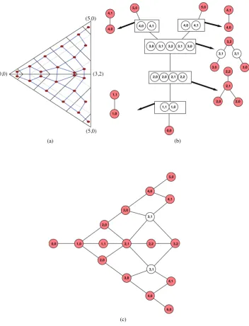
Figure 10: (a) The joint contour fragments and their adjacency graph for a PL-bivariate field defined by the values
{(5,0),(0,0),(5,0),(3,2)}at the vertices of a mesh of two triangles. (b) The Multi-Dimensional Reeb Graph constructed from the JCN. The critical nodes of the MDRG are the ‘red’ nodes which form the Jacobi structure. (c) Corresponding Joint Contour Net, with critical nodes from the MDRG marked in colour.
[image:22.595.123.476.170.632.2]Now the first step of the JCN algorithm constructs all the contour fragments corresponding to a quantization of each component field. In the second step, thejoint contour fragmentsare computed by computing the intersections of these contour fragments for the component fields in a cell. The third step is to construct an adjacency graph of these joint contour fragments where a node in the graph corresponds to a joint contour fragment and there is an edge between two nodes if the corresponding joint contour fragments are adjacent. Finally, the JCN is obtained by collapsing the neighbouring redundant nodes with identical isovalues. Thus, each node in the JCN corresponds to ajoint contour slab(orquantized fiber-component) and an edge represents the adjacency between two quantized fiber-components (with quantization levelmQ) of ef.
Note that one can build a multi-resolution JCN by increasing or decreasing the quantization level using a scaling factor for the ranges of the component fields. An example of a small JCN is given in Figure10, but we refer the interested reader to [6] for details. Next we show a convergence result of the JCN to the corresponding Reeb space in the limiting case when the quantization level increases and the domain-mesh becomes more refined.
6.2. Convergence
In the following, we consider the usual metrics for the Euclidean spaces and their subspaces. LetXbe a compactd-dimensional PL submanifold ofRd: in other words,Xis a closed bounded domain inRdwith piecewise linear boundary. Furthermore, let f:X→Rrbe a continuous map. LetMn,n≥1, be a sequence of meshes (i.e. triangulations) forXsuch thatMn+1is a subdi-vision ofMn,n≥1, and that
lim
n→∞diamMn=0,
where diamMnis the supremum of the diameters of all simplices ofMn.
Let f(n):X→Rr,n≥1, be the PL map defined as follows: on the vertices ofMn, f(n)
coincides with f, and on each simplex ofMn, f(n)is linear. We warn the reader thatf(n)may not
coincide with f even iff is PL andnis large, sinceMnmay contain small simplices that are not contained in a simplex of a simplicial decomposition ofXwith respect to which f is piecewise linear.
Letmk,k≥1, be an increasing sequence of quantization levels for f such thatmk+1is an ‘odd’ multiple ofmk,k≥1, and
lim
k→∞mk=∞.
Theorem 6.1. In the above situation, we have the following.
(1) For each n∈N(set of natural numbers or positive integers), the JCN of f(n)with respect
to Mnand mk, denoted by JCNn,k, canonically determines an r-dimensional cube complex g
JCNn,k in such a way that JCNn,kis its dual graph. Then,JCNgn,k converges to the Reeb spaceW
f(n) of f(n)(in the sense of “inverse limit”) when k→∞.
(2) The Reeb spaceW
f(n) converges toWf in a sense that{f(n)}n∈Nconverges uniformly to
f .
Remark. In many practical situations, we have a finite set of sample data of an unknown multi-field. In such situations, we can only analysef as a linear interpolation of the given sample data set. Thus, there exists a positive integerN0such that for alln≥N0, we have f = f(n). In such situations, our Theorem6.1gives a satisfactory answer.
Next we see that the simplification will have four stages: (i) extraction of the Jacobi structure from the JCN, (ii) computing regular and singular components for construction of the Reeb skeleton, (iii) computation of measures for each regular node in the Reeb skeleton, and (iv) simplification by pruning nodes corresponding to the “lip” components. In practice, the first stage is the most difficult - identifying the regular components, and this requires an intermediate data-structure, which we introduce now.
6.3. Multi-Dimensional Reeb Graphs
The first step in detecting and analysing the Jacobi structure is to identify the nodes in the JCN that capture changes in the topology - i.e. the quantized representatives of the Jacobi structure. To do so, we exploit a simple property of the JCN - that the slabs can be arranged hierarchically, with the levels of the hierarchy corresponding to the individual fields. At the highest level of the hierarchy, the slabs are only defined by field f1, and are therefore equivalent to interval volumes: as such, we can compute the Reeb graph for fieldf1(see Figure10(b)).
Algorithm 1CREATEREEBGRAPH(G,fi)
Input:A subgraphGofJCNand a chosen field fi
Output:The Reeb graphRGwith respect to field fi 1: Create Union-Find structureU F for fieldfi.
2: For each adjacentg1,g2∈Gwith fi(g1) =fi(g2), UFAdd(g1,g2) 3: for each componentClin UFdo
4: Create a nodenCl inRG
5: Map graph node-id(s) and field-values fromGtonCl
6: end for
7: Order nodesnC1, . . . ,nCn according to fifield values.
8: foredgee1e2inGdo
9: ife1,e2∈componentsCj,Ckand fi(e1),fi(e2)then 10: Add edgee(nCj,nCk)inRGif not already present
11: end if
12: end for
13: returnRG
Each slab (i.e. interval volume) of f1 can be broken up into smaller slabs with respect to field f2in a similar way (which form a subgraphGin the JCN), and the Reeb graph for these slabs computed similarly, as shown in Algorithm1. Proceeding recursively, we then compute a hierarchy of Reeb graphs, each of which represents the internal topology of a slab of the parent Reeb graph with respect to the child’s field. We call this hierarchy theMulti-Dimensional Reeb Graphor MDRG and denote this asMf.
Computing the MDRG is straightforward once the full JCN has been extracted: we start with the JCN and compute the Reeb graph for property f1by performing union-find processing over the nodes of the JCN. This breaks the JCN into subgraphs corresponding to slabs in the Reeb
graph of property f1. The MDRG for each subgraph is then computed recursively, and stored in the node of the parent Reeb graph to which its slab corresponds. In the process, the slabs get separated out into smaller and smaller components.
Algorithm 2MULTIDIMENSIONALREEBGRAPH(G,fi, . . . ,fr)
Input:GraphG, fields fi, . . . ,fr
Output:MDRGM
1: ifi≤rthen
2: LetR=CreateReebGraph(G,fi) 3: StoreRas root node ofM 4: forEach slabsofRdo
5: Extract subgraphGsof nodes ofGbelonging tosinR 6: ComputeMs=MultiDimensionalReebGraph(Gs,fi+1, . . . ,fr)
7: StoreMsat nodesofR
8: end for
9: returnM
10: else
11: returnM=/0 12: end if
We state this as an algorithm in Algorithm2and illustrate with a bivariate field in Figure10. This algorithm is stated recursively for simplicity, but can also be implemented with queue pro-cessing for speed. Moreover, the division of subgraphs at each level into slabs can be performed more efficiently by exploiting the connectivity already encoded in the JCN.
The principal value of the MDRG is that every node of the JCN in the Jacobi structure is guaranteed to be a critical node of the finest-resolution Reeb graphs (denoted as the critical nodes of the MDRG). This immediately gives a method of computing the Jacobi structure once the MDRG is known [39].
6.4. Jacobi Structure Extraction
Since every node belonging to the Jacobi structure is guaranteed to appear as a critical node of the lowest level of an MDRG, the initial stage in Jacobi structure extraction is simply to mark these nodes. Unmarked nodes are then guaranteed to be regular, and can be collected into regular components. Once this has been done, any remaining nodes that are adjacent to each other and to the same set of regular components are identified, as these form a 1-singular component between the regular components.
The first stage of this can be seen in Figure10, where the critical nodes of the lowest level of the MDRG together mark all of the Jacobi structure nodes in the JCN (in colour).
6.5. Reeb Skeleton Construction
(a) (b)
(c)
1
2 3
4
5 6
7 8
9
10
(d)
Figure 11: (a) Bivariate Field:(x2+y2−z,x2+y2+z2)in a box[−5,5]3, the ‘red’ components are the Jacobi set, (b)
the Joint Contour Net with the Jacobi structure (in red), (c) Regular Components, (d) the Reeb skeleton.
Now in the simplification algorithm, the order in which detachable Reeb skeleton nodes are removed is determined by the metrics associated with those nodes. Computation of such metrics are described next.
6.6. Computing Simplification Metrics
Our simplification algorithm can use any desired measure of importance for components of the Reeb space, including but not limited to:
• Range measure. As described in Subsection5.1, we can measure the size of the regular components by the induced measure of the range. This is easy to approximate - in this case, by the number of unique JCN slabs (i.e. pixels in the range) that map to a given regular component.
• Surface area. A regular component of the Reeb space is separated from other regular components by one or more singular components in the Jacobi structure. Since the regular components correspond to features and the singular components to boundaries between features, we can associate the area of the bounding surface with the regular component for the purpose of simplification. For the JCN, we can approximate this with the surface area of the fragments adjacent to the bounding region.
[image:26.595.151.445.138.420.2]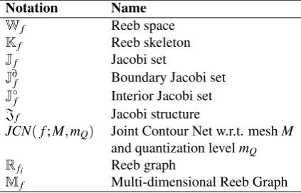
![Figure 1: (a) A stable bivariate field (f1, f2) ≡ (x2 + y2 + z2, z) from R3 to R2 that is visualized using the transparentisosurfaces of the first component field; black curves are the fiber-components of the bivariate field; the red line representsthe Jacobi set; (d) The Reeb space corresponding to (a) that is comprising one sheet (in pink) and the Jacobi structure (redparabolic curve); (b) The Jacobi set (consists of the red lines, top face and bottom face of the box) of the bivariate field(f1, f2) ≡ (x2 + y2, z) in the box [−1, 1] × [−1, 1] × [0, 1]; singular fibers passing through the boundary tangent pointsform a cylindrical surface that separates the domain into five components, denoted as A, B, C, D and E; (e) The Reebspace of the multi-field corresponding to (b) that is comprising five sheets (in grey) and the Jacobi structure (red lines);the regular components of the Reeb space are marked to match the corresponding components in the domain; componentsof the Jacobi set in the domain and their corresponding projections in the Reeb space are denoted by numbers; (c) Anunstable bivariate field (f1, f2) ≡ (x4 + y4 + z4 − 5(x2 + y2 + z2) + 10, z) from R3 to R2 that is visualized using thetransparent isosurfaces of the first component field; black curves are the fiber-components of the bivariate field; theJacobi set consists of 9 red lines; (f) The Reeb space corresponding to (c) that is comprising six sheets and the Jacobistructure (6 red lines).](https://thumb-us.123doks.com/thumbv2/123dok_us/7821849.173614/7.595.113.488.151.485/transparentisosurfaces-representsthe-corresponding-corresponding-corresponding-thetransparent-corresponding-jacobistructure.webp)