www.clim-past.net/12/663/2016/ doi:10.5194/cp-12-663-2016
© Author(s) 2016. CC Attribution 3.0 License.
The Pliocene Model Intercomparison Project (PlioMIP) Phase 2:
scientific objectives and experimental design
Alan M. Haywood1, Harry J. Dowsett2, Aisling M. Dolan1, David Rowley3, Ayako Abe-Ouchi4, Bette Otto-Bliesner5, Mark A. Chandler6, Stephen J. Hunter1, Daniel J. Lunt7, Matthew Pound8, and Ulrich Salzmann8
1School of Earth and Environment, University of Leeds, Woodhouse Lane, Leeds, LS2 9JT, UK
2Eastern Geology & Paleoclimate Science Center, US Geological Survey, MS 926A, 12201 Sunrise Valley Drive,
Reston, VA 20192, USA
3Department of Geophysical Sciences, University of Chicago, 5734 S. Ellis Avenue, Chicago, IL 60637, USA 4Center for Climate System Research (CCSR), University of Tokyo, Tokyo, Japan
5CCR, CGD/NCAR, PO Box 3000, Boulder, CO 80307-3000, USA
6NASA Goddard Institute for Space Studies, 2880 Broadway, New York, NY 10025, USA 7School of Geographical Sciences, University of Bristol, University Road, Bristol, BS8 1SS, UK
8Department of Geography, Faculty of Engineering and Environment, Northumbria University, Ellison Building,
Newcastle upon Tyne, NE1 8ST, UK
Correspondence to: Aisling M. Dolan ([email protected])
Received: 5 August 2015 – Published in Clim. Past Discuss.: 27 August 2015
Revised: 15 February 2016 – Accepted: 21 February 2016 – Published: 16 March 2016
Abstract. The Pliocene Model Intercomparison Project (PlioMIP) is a co-ordinated international climate modelling initiative to study and understand climate and environments of the Late Pliocene, as well as their potential relevance in the context of future climate change. PlioMIP examines the consistency of model predictions in simulating Pliocene cli-mate and their ability to reproduce clicli-mate signals preserved by geological climate archives. Here we provide a descrip-tion of the aim and objectives of the next phase of the model intercomparison project (PlioMIP Phase 2), and we present the experimental design and boundary conditions that will be utilized for climate model experiments in Phase 2.
Following on from PlioMIP Phase 1, Phase 2 will con-tinue to be a mechanism for sampling structural uncer-tainty within climate models. However, Phase 1 demon-strated the requirement to better understand boundary condi-tion uncertainties as well as uncertainty in the methodologies used for data–model comparison. Therefore, our strategy for Phase 2 is to utilize state-of-the-art boundary conditions that have emerged over the last 5 years. These include a new palaeogeographic reconstruction, detailing ocean bathymetry and land–ice surface topography. The ice surface topog-raphy is built upon the lessons learned from offline ice
sheet modelling studies. Land surface cover has been en-hanced by recent additions of Pliocene soils and lakes. Atmo-spheric reconstructions of palaeo-CO2 are emerging on
or-bital timescales, and these are also incorporated into PlioMIP Phase 2. New records of surface and sea surface temperature change are being produced that will be more temporally con-sistent with the boundary conditions and forcings used within models.
Finally we have designed a suite of prioritized experiments that tackle issues surrounding the basic understanding of the Pliocene and its relevance in the context of future climate change in a discrete way.
1 Introduction
1.1 PlioMIP Phase 1: design and objectives
production of boundary condition data sets suitable for use with numerical climate models.
Phase 1 of the PlioMIP project commenced in 2008 and was concluded in 2015. In Phase 1 two mid-Pliocene experi-ments were performed. Experiment 1 used atmosphere-only general circulation models (GCMs) with prescribed surface boundary conditions (sea surface temperatures, sea ice and vegetation) derived from the PRISM3D data set (Dowsett et al., 2010). Land–sea distribution and topography were also prescribed from PRISM3D. Experiment 2 used cou-pled ocean–atmosphere GCMs where sea surface tempera-tures and sea ice were predicted dynamically by the models; vegetation, land–sea distribution, and topography remained fixed to PRISM3D estimates.
The scientific objectives in Phase 1 were the following:
– examine large-scale features of mid-Pliocene climate that are consistent across models
– determine the dominant components of mid-Pliocene warming derived from the imposed boundary conditions
– examine first-order changes in ocean circulation be-tween the mid-Pliocene and present day
– examine the behaviour of the monsoons (e.g. their in-tensity)
– compare model results with proxy data to determine the performance of models simulating a warm climate state
– use the mid-Pliocene as a tool to evaluate the long-term sensitivity of the climate system to near-modern con-centrations of atmospheric CO2.
1.2 PlioMIP Phase 1 accomplishments
In the context of co-ordinated international model intercom-parison projects, PlioMIP achieved a number of firsts. For ex-ample, it was the first palaeoclimate modelling intercompar-ison project to require altered vegetation distributions to be modified in climate models, facilitating vegetation–climate feedbacks to be incorporated into the model intercompari-son. It was also the first intercomparison project that required individual groups to fully document the implementation of palaeo-boundary conditions within their models, along with the basic climatological responses. This was designed to fa-cilitate the intercomparison itself by enabling artefacts of in-dividual methodologies of boundary condition implementa-tion to be separated from robust model responses to imposed Pliocene boundary conditions. Through PlioMIP, a spin-off project known as PLISMIP (Pliocene Ice Sheet Model In-tercomparison Project; Dolan et al., 2012) was initiated and has focused on (1) assessing ice sheet model dependency of Greenland Ice Sheet reconstructions during the Pliocene us-ing shallow ice approximation ice sheet models (Dolan et al.,
2012; Koenig et al., 2015), (2) examining the effect of differ-ent GCM climatological forcing on predicted ice sheet con-figurations (Dolan et al., 2015) and (3) using shallow shelf ice sheet models for Antarctica to test both ice sheet model and climate model dependency on predicted ice sheet recon-structions (de Boer et al., 2015).
Outputs from PlioMIP Phase 1 include the following: – It identified consistency in surface temperature change
across models in the tropics and a lack of consistency in the simulated temperature response at high latitudes (Haywood et al., 2013a).
– Model predictions are inconsistent in terms of total pre-cipitation rate in the tropics (Haywood et al., 2013a). – Global annual mean surface temperatures increased by
1.8 to 3.6◦C and show a greater range for Experiment 2 using coupled ocean–atmosphere models than Exper-iment 1 using fixed sea surface temperatures (Haywood et al., 2013a).
– There was no clear indication in the model ensemble to support either enhanced or weaker Atlantic Meridional Overturning Circulation and ocean heat transport to the high latitudes (Z.-S. Zhang et al., 2013).
– Model predictions of enhanced Atlantic Meridional Overturning Circulation and ocean heat transport to high latitudes are inconsistent, in sign as well as strength (Z.-S. Zhang et al., 2013).
– Clear-sky albedo and greenhouse gas emissivity domi-nate polar amplification of surface temperature warm-ing durwarm-ing the Pliocene. This demonstrated the impor-tance of specified ice sheet and high-latitude vegeta-tion boundary condivegeta-tions and simulated sea ice and snow albedo feedbacks. Furthermore, the dominance of greenhouse gas emissivity in driving surface tempera-ture changes in the tropics was identified (Hill et al., 2014).
– The simulated weakened mid-Pliocene East Asian win-ter winds in north monsoon China and intensified East Asian summer winds in monsoon China agreed well with geological reconstructions (R. Zhang et al., 2013). – Data–model comparison using both sea surface and sur-face temperature proxies indicate that climate models potentially underestimate the magnitude of polar ampli-fication. However, current limitations in age control and correlation make interpreting data–model discrepancies challenging (Dowsett et al., 2012, 2013a; Salzmann et al., 2013).
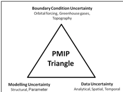
Figure 1.The PMIP triangle which illustrates three possible con-tributions to data–model discrepancy, and it has at its vertex model physics (structural and parameter uncertainty), model boundary conditions and proxy data uncertainty (Haywood et al., 2013a).
1.3 PlioMIP – emerging challenges/opportunities One of the key findings in PlioMIP Phase 1 was the poten-tial underestimation of model-predicted surface temperature warming in the high latitudes. Understanding data–model discord is non-trivial and can rarely be attributed to a single factor. The complexity of understanding data–model discord is highlighted by the PMIP triangle (Fig. 1), which illustrates three possible contributions to data–model discrepancy, and it has at its vertex model physics (structural and parameter uncertainty), model boundary conditions and proxy data un-certainty.
Following on from PlioMIP Phase 1, Phase 2 will continue to be a mechanism for sampling structural uncertainty within climate models as a suite of different models will take part in PlioMIP. However, Phase 1 demonstrated the requirement to better understand boundary condition uncertainties as well as weaknesses in the methodologies used for data–model com-parison, which largely stemmed from the time-averaged na-ture of proxy data used in previous data–model comparisons (Dowsett et al., 2013a; Salzmann et al., 2013). Therefore, our strategy for Phase 2 is to utilize state-of-the-art boundary conditions that have emerged over the last 5 years. These in-clude a new palaeogeography reconstruction detailing ocean bathymetry and land–ice surface topography and new data sets describing the distribution of Pliocene soils and lakes. The ice surface topography is built upon the lessons learned during the PLISMIP project (Dolan et al., 2015). Land sur-face cover will be enhanced by recent additions of Pliocene soils and lakes (Pound et al., 2014). Atmospheric reconstruc-tions of palaeo-CO2are emerging on orbital timescales (e.g.
Bartoli et al., 2011; Badger et al., 2013); these are also incor-porated into PlioMIP Phase 2.
It was recognized during Phase 1 that a key influence on data–model discord stems from uncertainties associated with the derivation of the proxy data sets used to assess the climate
models. Although certainty surrounding any proxy data set is limited by analytical, spatial and temporal uncertainty, Phase 1 highlighted temporal uncertainty as an important constraint on more robust methodologies for data–model comparison (DMC: Dowsett et al., 2013a; Haywood et al., 2013b; Salz-mann et al., 2013). The concept of climate stability during the Pliocene is overly simplistic both in geological climate archives and climate modelling approaches.
Due to the increasing recognition of climate variability in the Pliocene, time-averaged approaches to palaeoenviron-mental reconstruction have reached their ultimate potential to evaluate climate models. Therefore, enhancing the temporal resolution of data collection in order to more adequately un-derstand climate variation in the Pliocene is required, along with developing a more strategic approach to the choice of relevant Pliocene event(s) to reconstruct and model. One of PlioMIP’s guiding principles is to utilize palaeoenviron-ments to better inform us of likely scenarios for future global change. To this end, the event chosen for PlioMIP Phase 2 fo-cuses on the identification of a “time slice” centred on an in-terglacial peak (MIS KM5c; 3.205 Ma) that has near-modern orbital forcing, and yet it retains many of the characteristics of Pliocene warmth on which we have focused in the past (Dowsett et al., 2013b; Haywood et al., 2013b; Salzmann et al., 2013; Prescott et al., 2014). Discussions surround-ing potential modification of the LR04 benthic isotope stack (Lisiecki and Raymo, 2005) are currently ongoing, which may lead to a modification of the Marine Isotope Stage as-signed to the astrochronological age of 3.205.
PRISM and the wider Pliocene data community are ris-ing to the challenge to obtain higher-resolution proxy data that will inform the models about the chosen time slice (e.g. Dowsett et al., 2013b; see also Haywood et al., 2013b). The key differences between the PRISM data that underpinned PlioMIP Phase 1 and the new direction for data collection include the following:
– Expanding to a community-wide effort, new data gen-eration will focus on key locations and specific regions that have been identified by PlioMIP Phase 1 as impor-tant for understanding Pliocene climate variability and model performance.
– In order to increase our understanding of temporal changes in Pliocene climate, time series data are be-ing produced as standard, which will in essence increase previous temporal resolution by 2 orders of magnitude and lead to enhanced methods of data–model compari-son (Dowsett et al., 2013b).
Tier 1 Tier 2
PlioMIP Phase 2
Model evaluation
Tier 1
Tier 2
Understanding
CORE Pliocene timeslice
400
(Eoi ) Pre-industrial
280
(E ) Pliocene4Future
Pliocene4Pliocene
400
280 Pre-ind+plio
CO (E
)/ Pre-ind+plio
orog (Eo
)/ 2
280 Pre-ind+plio
ice (Ei
) Forcing factorisation
Forcing factorisation
280
400
Plio+pre-ind CO
(Eoi )/ Plio+pre-ind
orog (Ei
)/
2 400
Plio+pre-ind ice
(Eo )
400
Pre-industrial
CO 400
(E )
2
Pliocene CO 280
2
560
Pre-industrial CO 560 (E )2
450
Pliocene CO 450 (Eoi )2
350
Pliocene CO 350 (Eoi )2 450
Pliocene CO 450 (Eoi )2 280
(Eoi )
CMIP6 350
[image:4.612.128.469.65.283.2]Pliocene CO 350 (Eoi )2
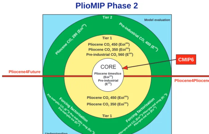
Figure 2.Experimental design strategy adopted for PlioMIP Phase 2. Core experiments will be completed by all model groups. Tier 1 and Tier 2 in either “Pliocene4Future” or “Pliocene4Pliocene” describe a series of sensitivity tests (Tier 1 being a higher priority for completion than Tier 2). Please note that Pliocene4Future Tier 1 experiment Pre-Industrial CO2400 also appears as a Tier 2 Pliocene4Pliocene exper-iment (Pre-Ind+PlioCO2). See Table 3 for the naming convention and further details of all PlioMIP Phase 2 experiments, as well as the
Supplement.
1.4 Pliocene4Future and Pliocene4Pliocene
The utilization of the mid-Pliocene as a means to understand future global change (“Pliocene4Future”) remains a prior-ity in Phase 2. It is our intention to forge stronger links be-tween PlioMIP, PMIP, CMIP and the next IPCC assessment. However, we recognize that many researchers are primar-ily interested in the Pliocene because it represents a con-siderable challenge to our understanding of the operation of the Earth system (“Pliocene4Pliocene”). Furthermore, a number of scientific requirements and priorities do not fit exclusively within a Pliocene4Future mandate. For exam-ple, palaeographic reconstructions are indicating more re-gional variations in palaeogeography than were appreciated in the past (Hill, 2015). Due to the differing requirements identified, in PlioMIP Phase 2 we have designed a portfo-lio of model experiments that effectively address both the “Pliocene4Future” and “Pliocene4Pliocene” agendas. This is illustrated in the following CMIP-style diagram (e.g. Tay-lor et al., 2012), where priorities for both agendas are high-lighted, with both agendas sharing a common core exper-iment that will serve as the PlioMIP Phase 2 experexper-iment within CMIP.
2 Strategy and methodology
2.1 Naming convention and summary of the experimental design for PlioMIP Phase 2
The experiments in PlioMIP Phase 2 have been grouped into halves “Pliocene4Pliocene” and “Pliocene4Future” and would ideally be completed by all participating groups. How-ever, only the core experiments must be completed by all groups. Each half of the project is divided into two “tiers” (Fig. 2). After the core experiments, Tier 1 experiments are identified as a higher priority for completion than Tier 2.
We describe several model simulations, which essentially consist of various combinations of boundary conditions as-sociated with prescribed CO2, orography, soils, lakes and ice
sheets. To simplify the experimental descriptions, we use the following nomenclature: Exc, where c is the concentration of CO2in ppmv, andx are any boundary conditions which are
Pliocene as opposed to pre-industrial, wherexcan be any or none of o, i, where o is orography and i is ice sheets. For example, a pre-industrial simulation with 280 ppmv CO2we
denoteE280. A Pliocene simulation with 400 ppmv is Eoi400, and a simulation with Pliocene ice sheets, but preindustrial orography, and at 560 ppmv, is Ei560. Note that in all our simulations, orography, lakes and soils are modified in uni-son, and so “o” denotes changes to orography, bathymetry, land–sea mask, lakes and soils combined.
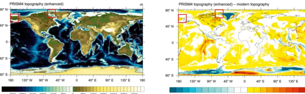
Figure 3.PRISM4 palaeogeography (enhanced) including topography/bathymetry (m) over the ice sheets (left). PRISM4 topographic and bathymetric anomaly (m) from modern (ETOPO1: right). Red boxes highlight the Canadian archipelago and Bering Strait as closed in both the standard and enhanced boundary condition data sets.
we have proposed simulations using 350 and 450 ppmv CO2
(Eoi350, Eoi450). Both these experiments will facilitate model evaluation using proxy data. Eoi450 enables the experimen-tal design to accommodate other Earth system processes that may have an effect on radiative forcing, besides greenhouse gas concentrations. For example, Unger and Yue (2014) have demonstrated that chemistry–climate feedbacks, in terms of their radiative forcing, may play as important, or even more important, role as CO2during the Pliocene. With a 450 ppmv
experiment we also aim to address how uncertainty in radia-tive forcing can account for high-latitude data–model mis-matches that were revealed in PlioMIP Phase 1 (Haywood et al., 2013a; Dowsett et al., 2012, 2013a; Salzmann et al., 2013). We have also specified a pre-industrial experiment with 560 ppmv CO2as a Tier 1 experiment (E560) to
facili-tate an investigation into climate (Charney) and Earth system sensitivity.
Within Tier 2 we have proposed two experiments that are designed to assess the dependence of climate sensitivity on the background climate and boundary condition states. Here we wish to compare the response of the system to CO2
forc-ing, between the Pliocene and the modern, by specifying a Pliocene experiment with 280 ppmv CO2(Eoi280), as well as
a pre-industrial experiment using 400 ppmv CO2(E400).
For our Pliocene4Pliocene agenda we have within Tier 1 focused on the atmospheric CO2 uncertainty by specifying
a higher- and lower-CO2 experiment at 450 and 350 ppmv
(Eoi450and Eoi350), which provides a 100 ppmv uncertainty bracket around our KM5c core experiment (using 400 ppmv CO2). Within Tier 2 we have specified a series of experiments
designed to identify the individual contribution of boundary condition changes to the overall modelled Pliocene climate response (E400,E280, Eo400, Eoi400). To assess non-linearity in the factorization of the forcings, we have specified an en-hanced factorization methodology (E400,E280, Eo400, Eo280, Ei400, Ei280, Eoi400, Eoi280: see Sect. 3.2).
2.2 Standard and enhanced boundary conditions All required boundary conditions can be accessed from the United States Geological Survey PlioMIP2 website (see http: //geology.er.usgs.gov/egpsc/prism/7_pliomip2.html). For the Pliocene experiment two versions of the palaeogeography (including land–sea mask (LSM), topography, bathymetry and ice distribution) are provided. The standard boundary condition data package does not require a modelling group to have the ability to alter the LSM or bathymetry (apart for selected regions of the Bering Strait, Canadian Archipelago and Hudson Bay). The enhanced boundary condition re-quires the ability to change the model’s LSM and ocean bathymetry more generally. The standard boundary condi-tion data set is provided in order to maximize the potential number of participating modelling groups. If groups are un-able to make any changes to their model’s LSM, then they may use their own LSM from their pre-industrial simulation. A PRISM4/PlioMIP Phase 2 modern land–sea mask is pro-vided to help guide the implementation of Pliocene topogra-phy into different climate models. Groups are asked to make every effort to implement as many of the boundary condi-tions in the enhanced data packages as possible; however, we recognize that this will not be possible for all groups.
2.3 Core experimental design and boundary conditions 2.3.1 Integration, atmospheric gases–aerosols, solar
constant–orbital configuration
400 ppmv. In the absence of proxy data, all other trace gases and aerosols are specified to be identical to the individual group’s pre-industrial control experiment.
While Pliocene CO2reconstruction is difficult, it is an
im-portant ongoing area of research with new records and syn-theses due to emerge over the next few years. Current evi-dence for Pliocene CO2comes from a number of sources:
(1) the stomatal density of fossil leaves (Kürschner et al., 1996), (2) carbon isotope analyses (e.g. Raymo et al., 1996), (3) alkenone-based estimates (Pagani et al., 2010; Seki et al., 2010; Badger et al., 2013) and (4) boron isotope anal-yses (e.g. Seki et al., 2010). For the warm intervals of the Pliocene values of CO2 from each of these proxies vary,
but within error they may overlap (Bartoli et al., 2011). The stomatal density records support a CO2concentration of 350
to 380 ppmv. The average of the Raymo et al. (1996) carbon isotope analyses is similar to the stomatal-based estimates, but peaks above that value (beyond 425 ppmv) occur. The Pagani et al. (2010) study reconstructed CO2 from a
num-ber of different marine records, and in three of the six ma-rine records a CO2value of 400 is reasonable and within the
range of 365 to 415 ppmv. In the Seki et al. (2010) study the alkenone-based CO2record is consistent with a value around
400 ppmv. Badger et al. (2013) have demonstrated that while absolute alkenone-based CO2reconstructions are influenced
by a number of factors, assessments of the degree of variabil-ity in CO2(rather than absolute concentration) are likely to
be more robust, and indicate less than 55 ppmv of variation between 3.3 and 2.8 million years ago. Atmospheric CO2
is an obvious choice for sensitivity tests as part of PlioMIP Phase 2 and is addressed within the experimental design for PlioMIP Phase 2. Information on the concentration of other greenhouse gasses such as methane and nitrogen dioxide is absent for the Pliocene and must therefore be prescribed at a pre-industrial level. The CO2concentrations specified within
PlioMIP Phase 2 are therefore designed to account for the total greenhouse gas forcing derived from all sources.
The solar constant is to be specified as the same as in each participating group’s pre-industrial control run. In previous versions, the PRISM boundary conditions (Dowsett et al., 2010) represented an average of the warm intervals during the time slab (∼3.3 to 3 million years), rather than condi-tions occurring during a discrete time slice. This made it im-possible to prescribe an orbital configuration that would be representative of the entire 300 000-year interval. However, due to the new focus within PRISM4 and PlioMIP Phase 2 to increase the temporal resolution of proxy records, and to concentrate on a smaller interval of time approaching a time slice reconstruction for MIS KM5c, it is now possible to pro-vide climate models with more certain values for astronom-ical and orbital forcing. The KM5c time slice was selected partly on the basis of a strong similarity in orbital forcing to present day. Therefore, in the interests of simplicity of the ex-perimental design, astronomical–orbital forcing in Pliocene experiments (eccentricity, obliquity, and precession) is to
re-main unchanged from each model’s pre-industrial control simulation.
2.3.2 Palaeogeography (land–sea mask, topography, bathymetry, ocean gateway land ice)
The PRISM4 palaeogeography provides a consistent recon-struction of topography, bathymetry, ice sheets and the land– sea mask that can be implemented in PlioMIP Phase 2 models. The PRISM4 Pliocene palaeogeography data set is provided in NetCDF format at a 1◦×1◦ resolution. The PRISM4 palaeogeography includes components such as the contribution of dynamic topography caused by changes in the mantle flow (e.g. Rowley et al., 2013) and the glacial iso-static response of loading specific Pliocene ice sheets (e.g. Raymo et al., 2011), which were not previously consid-ered in the PRISM3D reconstruction of Sohl et al. (2009). In the standard boundary condition data set all ocean gate-ways remain the same as the modern except for the Bering Strait, which should be closed, and the Canadian Arctic Archipelago, which should also be closed (isolating Baffin Bay and the Labrador Sea from the Arctic Ocean). In the enhanced boundary condition data set the Bering Strait and Canadian Arctic Archipelago are closed, but there are other required changes in the Torres Strait, Java Sea, South China Sea, Kara Strait, as well as a West Antarctic seaway.
The approach taken to derive PRISM4 ice sheets in the palaeogeography reconstruction is different to PRISM3D (Dowsett et al., 2010). The results of PLISMIP have shown that ice sheet model dependency over Greenland is low. How-ever, the initial climatological forcing has a large impact on the predicted Greenland Ice Sheet configuration (Dolan et al., 2015; Koenig et al., 2015). Using a compilation of the re-sults presented in Koenig et al. (2015), we have implemented an ice sheet configuration over Greenland in PRISM4 where we have the highest confidence in the possibility of ice sheet location during the warmest parts of the Late Pliocene (see Fig. 6b in Koenig et al., 2015). The reconstruction of Keonig et al. (2015) was modified by removing ice from southern Greenland. The presence of ice in that region is inconsistent with palynological studies that suggest that southern Green-land was vegetated during warm intervals of the Pliocene (e.g. de Vernal and Mudie, 1989). The PRISM4 Greenland Ice Sheet configuration is smaller than in PRISM3D, and ice is limited to high elevations in the East Greenland Mountains (Fig. 4).
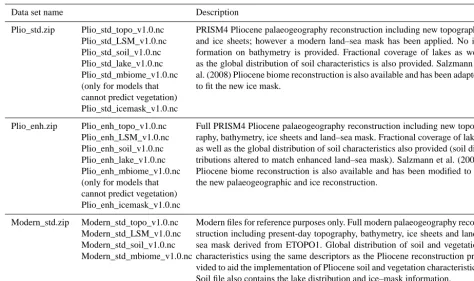
Table 1.Details of NetCDF data packages provided to facilitate PlioMIP Phase 2 experiments.
Data set name Description
Plio_std.zip Plio_std_topo_v1.0.nc Plio_std_LSM_v1.0.nc Plio_std_soil_v1.0.nc Plio_std_lake_v1.0.nc Plio_std_mbiome_v1.0.nc (only for models that cannot predict vegetation) Plio_std_icemask_v1.0.nc
PRISM4 Pliocene palaeogeography reconstruction including new topography and ice sheets; however a modern land–sea mask has been applied. No in-formation on bathymetry is provided. Fractional coverage of lakes as well as the global distribution of soil characteristics is also provided. Salzmann et al. (2008) Pliocene biome reconstruction is also available and has been adapted to fit the new ice mask.
Plio_enh.zip Plio_enh_topo_v1.0.nc Plio_enh_LSM_v1.0.nc Plio_enh_soil_v1.0.nc Plio_enh_lake_v1.0.nc Plio_enh_mbiome_v1.0.nc (only for models that cannot predict vegetation) Plio_enh_icemask_v1.0.nc
Full PRISM4 Pliocene palaeogeography reconstruction including new topog-raphy, bathymetry, ice sheets and land–sea mask. Fractional coverage of lakes as well as the global distribution of soil characteristics also provided (soil dis-tributions altered to match enhanced land–sea mask). Salzmann et al. (2008) Pliocene biome reconstruction is also available and has been modified to fit the new palaeogeographic and ice reconstruction.
Modern_std.zip Modern_std_topo_v1.0.nc Modern_std_LSM_v1.0.nc Modern_std_soil_v1.0.nc Modern_std_mbiome_v1.0.nc
Modern files for reference purposes only. Full modern palaeogeography recon-struction including present-day topography, bathymetry, ice sheets and land– sea mask derived from ETOPO1. Global distribution of soil and vegetation characteristics using the same descriptors as the Pliocene reconstruction pro-vided to aid the implementation of Pliocene soil and vegetation characteristics. Soil file also contains the lake distribution and ice–mask information.
that the Wilkes subglacial basin may have been highly dy-namic during the warmest parts of the Late Pliocene, and they infer significant potential for ice sheet retreat in this re-gion. Additionally, Young et al. (2011) highlight the Aurora subglacial basin as an area which may have been subject to marine ice sheet instabilities in the past (potentially in the Pliocene). Therefore, over East Antarctica PlioMIP Phase 2 uses the PRISM3D ice sheet reconstruction (Hill et al., 2007; Hill, 2009; Dowsett et al., 2010), as this remains consis-tent with more recently available data. In this reconstruction (Fig. 4) large portions of the East Antarctic ice sheet show little change or a small increase in surface altitude with re-spect to modern, and significant ice sheet retreat is limited to the low-lying Wilkes and Aurora subglacial basins.
For the Pliocene experiments, two versions of the palaeo-geography will be provided to climate modelling groups:
– Standard: For the models where altering the LSM and bathymetry is problematic, we provide a palaeo-geography with a modern land–sea configuration and bathymetry (apart from in the Hudson Bay, Bering Strait and Canadian Archipelago). In this instance the Late Pliocene topographic elevations were extended to the modern coastline, and the bathymetry remained at mod-ern values. Groups that are unable to change their land– sea mask or bathymetry at all are asked to use their lo-cal modern boundary conditions; however guidance on the implementation of Pliocene topography in this case
Figure 4. PRISM4 land–sea mask (enhanced version) show-ing Greenland and Antarctic ice sheet distribution. Canadian archipelago and Bering Strait closed (red boxes) in both the stan-dard and enhanced boundary condition data sets.
should be taken from the standard palaeogeography data set.
– Enhanced: This presents the full palaeogeographic reconstruction including all changes to topography, bathymetry, ice sheets and the LSM.
[image:7.612.310.548.385.534.2]differ-ences in the models themselves rather than the differdiffer-ences of modern boundary conditions, it has been decided to implement Pliocene topography (and bathymetry) as an anomaly to whatever modern topographic data set is used by each modelling group in their own model. To create the Pliocene topography (and bathymetry) the difference be-tween the PRISM4 Pliocene and PRISM4 Modern topog-raphy (bathymetry) should be calculated and added to the modern topographic (bathymetric) data sets each participat-ing modellparticipat-ing group employs within their own pre-industrial control simulations, such that
PlioTOPO=PRISM4PlioTOPO−PRISM4ModernTOPO
+ModernTOPO Local and
PlioBATH=PRISM4PlioBATH−PRISM4ModernBATH
+ModernBATH Local.
With this formulation it is possible that on occasion grid cells may become land where the intention is for an ocean cell to be specified and vice versa. In this case the specified Pliocene LSM takes precedence. In other words this ensure that the integrity of Pliocene LSM boundary condition data is always preserved. Data sets to be provided at a 1◦×1◦resolution for the core experiments can be found in Table 1.
2.3.3 Vegetation, lakes, soils and rivers
A global data set of vegetation for the KM5c time slice is not available. A number of climate models now have the abil-ity to simulate the type and distribution of vegetation us-ing dynamic vegetation models. In PlioMIP Phase 2 vege-tation models should be initialized with pre-industrial veg-etation cover and spun up until an equilibrium condition is reached. If Pliocene vegetation cannot be predicted dy-namically, modelling groups can prescribe vegetation using the Salzmann et al. (2008) PRISM3 vegetation reconstruc-tion used within PlioMIP Phase 1 (Haywood et al., 2010, 2011) and provided as a mega biome reconstruction in the PlioMIP Phase 2 boundary condition files. An equivalent po-tential natural vegetation data set is also provided to guide how groups implement prescribed Pliocene vegetation. Fur-ther details on correctly approaching the implementation of prescribed Pliocene vegetation for PlioMIP Phase 2 can be found in Haywood et al. (2010: Sect. 3.5).
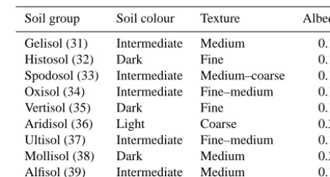
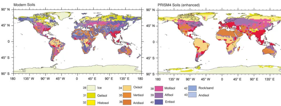
[image:8.612.312.543.104.228.2]Due to lack of information covering the distribution of lakes and soils during PlioMIP Phase 1, lakes were absent from the land cover boundary conditions. Since PlioMIP Phase 1, the global distribution of Late Pliocene soils and lakes has been reconstructed through a synthesis of geolog-ical data (Pound et al., 2014). Initial experiments using the Hadley Centre Coupled Climate Model Version 3 (HadCM3) indicate regionally confined changes of local climate and
Table 2.The colour (for albedo) and texture translations for the soil orders used in the modelling of Late Pliocene soils, based upon HadCM3 classification.
Soil group Soil colour Texture Albedo
Gelisol (31) Intermediate Medium 0.17
Histosol (32) Dark Fine 0.11
Spodosol (33) Intermediate Medium–coarse 0.17 Oxisol (34) Intermediate Fine–medium 0.17
Vertisol (35) Dark Fine 0.11
Aridisol (36) Light Coarse 0.35
Ultisol (37) Intermediate Fine–medium 0.17
Mollisol (38) Dark Medium 0.35
Alfisol (39) Intermediate Medium 0.17
vegetation in response to the new lake and soil boundary conditions (Pound et al., 2014). When combined (lakes plus soils), the feedbacks on climate from Late Pliocene lakes and soils improve the proxy data–model fit in western North America as well as the southern part of northern Africa (Pound et al., 2014).
In PlioMIP Phase 2 all modelling groups should imple-ment the Pound et al. (2014) data sets for global lake (Fig. 5) and soil distribution (Fig. 6). If lake distribution is a dynam-ically predicted variable within a model (i.e. lake distribu-tions can change as a result of predicted changes in climate), prescribing the Pound et al. (2014) lake data set is not nec-essary. The lake data set provides information on both lake size as well as the fractional coverage of lakes within model grid boxes. Figure 5 also shows how the lake distribution and sizes differ from modern, most notably the absence of post-glacial lakes in North America and the presence of large lakes in central Africa (Pound et al., 2014).
The colour (for albedo) and texture translations for the nine soil orders used in the modelling of Late Pliocene soils and lakes are provided to guide the implementation of soil type and distribution in models. This translation is based upon the definition of soils with the HadCM3 (Table 2).
Figure 5. Modern and Pliocene (PRISM4) fractional lake coverage data set (Pound et al., 2014). Modern data are based upon the FAO/UNESCO modern soil map (Version 3.6).
Figure 6.Pound et al. (2014) data set of global modern and Pliocene soil types (shown on the enhanced PlioMIP2 land–sea mask). Modern data are based upon the FAO/UNESCO modern soil map (Version 3.6).
With regard to river routing the required solution is to fol-low modern river routes except where this would be inap-propriate due to the appearance of new land grid cells in the Pliocene land–sea mask, in which case rivers should be routed to the nearest ocean grid box or most appropriate river outflow point.
3 Sensitivity experiments and forcing factorization
3.1 Sensitivity experiments 3.1.1 Pliocene4Future Tier 1 and 2
Within the Pliocene4Future agenda a pre-industrial exper-iment with 560 ppmv CO2 has been selected as a Tier
1 experiment (E560). This is to facilitate an investigation into climate (Charney) and Earth system sensitivity. Also given the uncertainty in total greenhouse gas forcing for
the KM5c time slice, we have proposed a simulation using 450 and 350 ppmv CO2 (Eoi450, Eoi350). Within Tier 2 we
have proposed two experiments that are designed to assess the similarity of Pliocene and future climate feedbacks to higher CO2levels by specifying a Pliocene experiment using
280 ppmv CO2(Eoi280) as well as pre-industrial experiment
using 400 ppmv (E400).
3.1.2 Pliocene4Pliocene Tier 1
For the Pliocene4Pliocene agenda we have within Tier 1 fo-cused on the atmospheric CO2 uncertainty by specifying a
high- and low-CO2experiment at 450 and 350 ppmv (Eoi450
[image:9.612.54.548.270.457.2]Table 3.Details of all experiments proposed in PlioMIP Phase 2.
ID Description LSM3,4 Topo. Soils Lakes Ice Vegetation5 CO7
2 Status: Tier 1 or 2
(T) & P4F/P4P6
E280 Pre-industrial experiment as per Modern Modern Modern Modern Modern Dynamic 280 CORE control simulation in PlioMIP2 experiment.
E400 Pre-industrial experiment as per control simulation Modern Modern Modern Modern Modern Dynamic 400 T2: P4F – T2: P4P
in core PlioMIP2 experiment – CO2400 ppmv.
E560 Pre-industrial experiment as per control Modern Modern Modern Modern Modern Dynamic 560 T1: P4F
simulation in core PlioMIP2 experiment – CO2560 ppmv.
Eo280 Pre-industrial experiment as per control simulation in core PlioMIP2 experiment; Modern Pliocene Pliocene Pliocene Modern Dynamic 280 T2: P4P
however topography (including soils and lakes) is set to Pliocene values outside of ice sheet regions. The land masses of Greenland and Antarctica should have pre-industrial boundary conditions (see Fig. S1a).
Ei280 Pre-industrial experiment as per control Modern Modern Modern Modern Pliocene Dynamic 280 T2: P4P
simulation in core PlioMIP2 experiment; however the ice configurations
on Greenland and Antarctica are set to be Pliocene.6
Eo400 Pliocene experiment as per control simulation Modern Pliocene Pliocene Pliocene Modern Dynamic 400 T2: P4P
in core PlioMIP2 experiment; however ice sheets on Greenland and Antarctica set to modern.
Ei400 Pliocene experiment as per control simulation in Modern Modern Modern Modern Pliocene Dynamic 400 T2: P4P
Core PlioMIP2 experiment. Topography outside of the ice sheet regions set to modern. Soils and lakes are also modern in this experiment.
Eoi280 Pliocene experiment as per control simulation Modern Pliocene Pliocene Pliocene Pliocene Dynamic 280 T2: P4P – T2: P4F
in Core PlioMIP2 experiment – CO2280 ppmv
Eoi400 Pliocene experiment as per control Pliocene–Modern Pliocene Pliocene Pliocene Pliocene Dynamic 400 CORE
simulation in Core PlioMIP2 experiment.
Eoi450 Pliocene experiment as per control simulation Pliocene–Modern Pliocene Pliocene Pliocene Pliocene Dynamic 450 T1: P4F – T1: P4P
in Core PlioMIP2 experiment – CO2450 ppmv
Eoi350 Pliocene experiment as per control simulation in Pliocene–Modern Pliocene Pliocene Pliocene Pliocene Dynamic 350 T1: P4F – T1: P4P
Core PlioMIP2 experiment, but with CO2set to 350 ppmv
1By ice sheet regions we mean the land masses of Greenland and Antarctica (not the areas of ice specified within the ice masks).2Where ice retreat (i.e. the change from pre-industrial ice to Pliocene ice) leaves information gaps in soils, please extrapolate modern soil
values from nearest grid square.3For experiments Eoi400, Eoi350and Eoi450this may be using the standard or enhanced Pliocene LSM.4For simplicity of approach we assume that all forcing factorization experiments will only use the standard rather than enhanced data sets.5Prescribed static vegetation is also an option. Bold text indicates core experiments (compulsory), all other experiments are optional.6P4F indicates Pliocene4Future; P4P indicates Pliocene for Pliocene. See also the Supplement.7CMIP6 groups should set the
atmospheric CO2levels in their PlioMIP2 pre-industrial experiments to the same as in their CMIP6 DECK pre-industrial simulation. Note that the CMIP6 1850 CO2is slightly higher than 280 ppm, so the radiative forcing difference with the PlioMIP2 higher CO2
experiments will not be exactly the same as those of non-CMIP6 groups that specify pre-industrial CO2at 280 ppm.
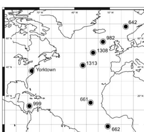
Figure 7.Initial PRISM4 sites being investigated to generate time slice proxy data for model evaluation in PlioMIP Phase 2.
3.2 Pliocene4Pliocene Tier 2: forcing factorization experiments
The primary aim of the Pliocene4Pliocene Tier 2 forcing fac-torization experiments is to assess the relative importance of various boundary condition changes which contribute to Pliocene warmth. Following a similar methodology adopted in Lunt et al. (2012) we intend to partition the total Pliocene
warming (or temperature change; 1T) into three compo-nents, each due to the change in one of the following bound-ary conditions: CO2, topography or ice sheets. Our
factor-ization, which is that proposed by Lunt et al. (2012), can be written as follows:
1T =dTCO2+dTtopo+dTice
dTCO2=1/4(E400−E280)+(Eo400−Eo280)
+(Ei400−Ei280)+(Eoi400−Eoi280) dTorog=1/4(Eo280−E280)+(Eo400−E400)
+(Eoi280−Ei280)+(Eoi400−Ei400) dTice=1/4(Ei280−E280)+(Ei400−E400)
+(Eoi280−Eo280)+(Eoi400−Eo400).
This gives a total of eight simulations required (2N, whereN
is the number of processes factorized,=3 in this case), al-though only five of them (Eo400, Eo280, Ei400, Ei280, Eoi280)
[image:10.612.49.285.356.571.2]are in addition to simulations already in Tier 1 or the core. This method, although more computationally demanding than the linear approach (e.g. Broccoli and Manabe, 1987; von Deimling et al., 2006), has the advantage that it takes into account non-linear interactions, is symmetric and is unique (Table 3).
If groups do not have the computational resource to carry out the full factorization, they may carry out a linear factor-ization, as follows:
dTCO2=E400−E280
dTice=Eoi400−Eo400.
This is a total of four simulations, but only one of them (Eo400) is in addition to simulations already in Tier 1 or the core. Further guidance on boundary condition implementa-tion for the forcing factorizaimplementa-tion experiment can be found in Fig. S1 in the Supplement.
4 Proxy data for the evaluation of model outputs
Short, high-resolution time series extending from MIS M2 through KM3 will be necessary to meet the evaluation re-quirements of PlioMIP Phase 2. Marine sequences will de-pend upon chronology from the Lisiecki and Raymo 2005 (LR04) timescale and should have multiple palaeoenviron-mental proxies (Dowsett et al., 2013a). Previous work from the palaeoclimate data community suggests a number of sites potentially suitable for evaluation of PlioMIP Phase 2 model outputs (e.g. Dowsett et al., 2013a, b; Fedorov et al., 2013; Salzmann et al., 2013, Brigham-Grette et al., 2013). Well-dated, high-resolution records from the con-tinental interior are scarce, and terrestrial reconstructions will be mostly based on marine and marginal marine se-quences. The primary areas of discord between simulated and estimated Pliocene palaeoclimate conditions identified in PlioMIP Phase 1 include the mid-to-high-latitude North Atlantic, tropics and upwelling regions (Dowsett et al., 2012). The PRISM4 marine and terrestrial contribution to the PlioMIP Phase 2 community evaluation data set has been ini-tially concentrated in the North Atlantic region (Fig. 7).
5 Variables, output format, data processing and storage
If the PlioMIP Phase 2 core experiment is adopted as a CMIP6 simulation, model data for this experiment must use the Climate Model Output Rewriter (CMOR) format and be stored on an ESGF node (The Earth System Grid Federation). The CMOR library has been specially devel-oped to help meet the requirements of the model inter-comparison. Further details of CMIP6 experiments and re-quired outputs/CMOR file formats will be made available on the CMIP6 website (http://www.wcrp-climate.org/index. php/wgcm-cmip/wgcm-cmip6).
If the PlioMIP Phase 2 core experiment is specified as a PMIP core experiment, the same guidelines for output format and storage of data detailed for CMIP6 apply. For PlioMIP Phase 2 experiments listed within Tier 1 and Tier 2, more flexibility in terms of data storage and file formats is avail-able. PlioMIP Phase 2 has modified the established variable list outlined by the third phase of the PMIP project. The list of required variables can be found on the PlioMIP Phase 2 website (http://geology.er.usgs.gov/egpsc/prism/7_pliomip2. html). All model outputs will be submitted initially to a data repository at the University of Leeds (including the PlioMIP
Phase 2 core experiment, which may have data replicated in CMOR format on an ESGF node). Requests for access should be sent to A. Haywood. In general (CMIP6 guidelines aside) PlioMIP project requires participants to prepare their data files so that they meet the following constraints (regard-less of the way their models produce and store their results). – The data files have to be in the (now widely used) NetCDF binary file format and conform to the CF (Cli-mate and Forecast) metadata convention (outlined on the website http://cf-pcmdi.llnl.gov/).
– There must be only one output variable per file.
– For the data that are a function of longitude and lati-tude, only regular grids (grids representable as a Carte-sian product of longitude and latitude axes) are allowed. – The file names have to follow the PMIP2 file name
con-vention and be unique (see the PMIP2 website).
The Supplement related to this article is available online at doi:10.5194/cp-12-663-2016-supplement.
Acknowledgements. A. M. Haywood, A. M. Dolan and S. J. Hunter acknowledge that the research leading to these results has received funding from the European Research Council under the European Union’s Seventh Framework Programme (FP7/2007-2013)/ERC grant agreement no. 278636, as well as the EPSRC-supported Past Earth Network. U. Salzmann, A. M. Haywood and M. J. Pound acknowledge funding received from the Natural Environment Research Council (NERC Grant NE/I016287/1). A .M. Haywood and D. J. Lunt acknowledge funding received from the Natural Environment Research Council (NERC Grant NE/G009112/1). D. J. Lunt acknowledges NERC grant NE/H006273/1. H. J. Dowsett recognizes the continued sup-port of the United States Geological Survey Climate and Land Use Change Research and Development Program. B. L. Otto-Bliesner recognizes the continued support of the National Center for Atmo-spheric Research, which is sponsored by the US National Science Foundation. M. A. Chandler is supported by the NASA Modeling, Analysis, and Prediction program (NASA Grant NNX14AB99A) and the NASA High-End Computing (HEC) Program through the NASA Center for Climate Simulation (NCCS) at Goddard Space Flight Center.
Edited by: W.-L. Chan
References
Bartoli, G., Honisch, B. R., and Zeebe, R. E.: Atmospheric CO2 decline during the Pliocene intensification of
North-ern Hemisphere glaciations, Paleoceanography 26, PA4213, doi:10.1029/2010PA002055, 2011.
Brigham-Grette, J., Melles, M., Minyuk, P., Andreev, A., Tarasov, P., DeConto, R., Koenig, S, Nowaczyk, N., Wennrich, V., Rosen, P., Haltia-Hovi, E., Cook, T., Gebhardt, T., Meyer-Jacob, C., Sny-der, J., and Herzschuh, U.: Pliocene Warmth, Polar Amplifica-tion, and Stepped Pleistocene Cooling Recorded in NE Arctic Russia, Science, 340, 1421–1427, 2013.
Broccoli, A. J. and Manabe, S.: The influence of continental ice, at-mospheric CO2, and land albedo on the climate of the last glacial
maximum, Clim. Dynam., 1, 87–99, 1987.
Cook C. P., Hill, D. J., Van De Flierdt, T., Williams, T., Hemming, S. R., Dolan, A. M., Pierce, E. L., Escutia, C., Harwood, D., Cortese, G., and Gonzales, J. J.: Sea surface temperature control on the distribution of far-travelled Southern Ocean ice-rafted de-tritus during the Pliocene, Paleoceanography, 29, 533–548, 2014. de Boer, B., Dolan, A. M., Bernales, J., Gasson, E., Goelzer, H., Golledge, N. R., Sutter, J., Huybrechts, P., Lohmann, G., Rogozhina, I., Abe-Ouchi, A., Saito, F., and van de Wal, R. S. W.: Simulating the Antarctic ice sheet in the late-Pliocene warm period: PLISMIP-ANT, an ice-sheet model intercompar-ison project, The Cryosphere, 9, 881–903, doi:10.5194/tc-9-881-2015, 2015.
De Vernal, A. and Mudie, P. J.: Pliocene and Pleistocene palynos-tratigraphy of at ODP Sites 646 and 647, eastern and southern Labrador Sea, in: Proceedings of the Ocean Drilling Program, edited by: Srivastava, S. P., Arthur, M., Clement, B., et al., Sci-entific Results, 10, 401–422, 1989.
Dolan, A. M., Koenig, S. J., Hill, D. J., Haywood, A. M., and DeConto, R. M.: Pliocene Ice Sheet Modelling Intercomparison Project (PLISMIP) – experimental design, Geosci. Model Dev., 5, 963–974, doi:10.5194/gmd-5-963-2012, 2012.
Dolan, A. M., Hunter, S. J., Hill, D. J., Haywood, A. M., Koenig, S. J., Otto-Bliesner, B. L., Abe-Ouchi, A., Bragg, F., Chan, W.-L., Chandler, M. A., Contoux, C., Jost, A., Kamae, Y., Lohmann, G., Lunt, D. J., Ramstein, G., Rosenbloom, N. A., Sohl, L., Stepanek, C., Ueda, H., Yan, Q., and Zhang, Z.: Using results from the PlioMIP ensemble to investigate the Greenland Ice Sheet dur-ing the mid-Pliocene Warm Period, Clim. Past, 11, 403–424, doi:10.5194/cp-11-403-2015, 2015.
Dowsett, H., Robinson, M., Haywood, A., Salzmann, U., Hill, D., Sohl, L., Chandler, M., Williams, M., Foley, K., and Stoll, D.: The PRISM3D paleoenvironmental reconstruction, Stratigraphy, 7, 123–139, 2010.
Dowsett, H. J., Robinson, M. M., Haywood, A. M., Hill, D. J., Dolan, A. M., Stoll, D. K., Chan, W.-L., Abe-Ouchi, A., Chan-dler, M. A., and Rosenbloom, N. A.: Assessing confidence in Pliocene sea surface temperatures to evaluate predictive models, Nature Climate Change, 2, 365–371, 2012.
Dowsett, H. J., Foley, K. M., Stoll, D. K., Chandler, M. A., Sohl, L. E., Bentsen, M., Otto-Bliesner, B. L., Bragg, F. J., Chan, W.-L., Contoux, C., Dolan, A. M., Haywood, A. M., Jonas, J. A., Jost, A., Kamae, Y., Lohmann, G., Lunt, D. J., Nisancioglu, K. H., Abe-Ouchi, A., Ramstein, G., Riesselman, C. R., Robinson, M. M., Rosenbloom, N. A., Salzmann, U., Stepanek, C., Strother, S. L., Ueda, H., Yan, Q., and Zhang, Z.: Sea Surface Temperature
of the mid-Piacenzian Ocean: A Data-Model Comparison, Sci. Rep. Res. Tohoku A, 3, 1–8, 2013a.
Dowsett, H. J., Robinson, M. M., Stoll, D. K., Foley, K. M., John-son, A. L. A., Williams, M., and Riesselman, C. R.: The PRISM (Pliocene Palaeoclimate) reconstruction: Time for a paradigm shift, Philos. T. R. Soc. A, 371, 1–24, 2013b.
Fedorov, A., Brierley, C., Lawrence, K., Liu, Z., Dekens, P., and Ravelo, A.: Patterns and mechanisms of early Pliocene warmth, Nature, 496, 43–49, 2013.
Haywood, A. M., Dowsett, H. J., Otto-Bliesner, B., Chandler, M. A., Dolan, A. M., Hill, D. J., Lunt, D. J., Robinson, M. M., Rosen-bloom, N., Salzmann, U., and Sohl, L. E.: Pliocene Model Inter-comparison Project (PlioMIP): experimental design and bound-ary conditions (Experiment 1), Geosci. Model Dev., 3, 227–242, doi:10.5194/gmd-3-227-2010, 2010.
Haywood, A. M., Dowsett, H. J., Robinson, M. M., Stoll, D. K., Dolan, A. M., Lunt, D. J., Otto-Bliesner, B., and Chandler, M. A.: Pliocene Model Intercomparison Project (PlioMIP): experi-mental design and boundary conditions (Experiment 2), Geosci. Model Dev., 4, 571–577, doi:10.5194/gmd-4-571-2011, 2011. Haywood, A. M., Hill, D. J., Dolan, A. M., Otto-Bliesner, B. L.,
Bragg, F., Chan, W.-L., Chandler, M. A., Contoux, C., Dowsett, H. J., Jost, A., Kamae, Y., Lohmann, G., Lunt, D. J., Abe-Ouchi, A., Pickering, S. J., Ramstein, G., Rosenbloom, N. A., Salz-mann, U., Sohl, L., Stepanek, C., Ueda, H., Yan, Q., and Zhang, Z.: Large-scale features of Pliocene climate: results from the Pliocene Model Intercomparison Project, Clim. Past, 9, 191–209, doi:10.5194/cp-9-191-2013, 2013a.
Haywood, A. M., Dolan, A. M., Pickering, S. J., Dowsett, H. J., Mc-Clymont, E. L., Prescott, C. L., Salzmann, U., Hill, D. J., Hunter, S. J., and Lunt, D. J.: On the identification of a Pliocene time slice for data–model comparison, Philos. T. R. Soc. A, 371, 2001, doi:10.1098/rsta.2012.0515, 2013b.
Hill, D. J.: Modelling Earth’s Cryosphere during Pliocene Warm Peak, PhD thesis, University of Bristol, 2009.
Hill, D. J.: The non-analogue nature of Pliocene temperature gradi-ents, Earth Planet. Sc. Lett., 425, 232–241, 2015.
Hill, D. J., Haywood, A. M., Hindmarsh, R. C. A., and Valdes, P. J.: Characterizing ice sheets during the Pliocene: evidence from data and models Deep time perspectives on climate change: marrying the signals from computer models and biological proxies, edited by: Williams, M., Haywood, A. M., Gregory, D., and Schmidt, D. N., London, UK, Micropalaeontological Society, Special Publi-cation, Geological Society of London, 517–538, 2007.
Hill, D. J., Haywood, A. M., Lunt, D. J., Hunter, S. J., Bragg, F. J., Contoux, C., Stepanek, C., Sohl, L., Rosenbloom, N. A., Chan, W.-L., Kamae, Y., Zhang, Z., Abe-Ouchi, A., Chan-dler, M. A., Jost, A., Lohmann, G., Otto-Bliesner, B. L., Ram-stein, G., and Ueda, H.: Evaluating the dominant components of warming in Pliocene climate simulations, Clim. Past, 10, 79–90, doi:10.5194/cp-10-79-2014, 2014.
Koenig, S. J., Dolan, A. M., de Boer, B., Stone, E. J., Hill, D. J., De-Conto, R. M., Abe-Ouchi, A., Lunt, D. J., Pollard, D., Quiquet, A., Saito, F., Savage, J., and van de Wal, R.: Ice sheet model dependency of the simulated Greenland Ice Sheet in the mid-Pliocene, Clim. Past, 11, 369–381, doi:10.5194/cp-11-369-2015, 2015.
Pleis-tocene paleoatmospheric CO2concentrations, Mar. Micropale-ontol., 27, 299–312, 1996.
Lisiecki, L. E. and Raymo, M. E.: A Pliocene-Pleistocene stack of 57 globally distributed benthic d18O records, Paleoceanography, 20, PA1003, doi:10.1029/2004PA001071, 2005.
Lunt, D. J., Haywood, A. M., Schmidt, G. A., Salzmann, U., Valdes, P. J., Dowsett, H. J., and Loptson C. A.:On the causes of mid-Pliocene warmth and polar amplification, Earth Planet. Sci. Lett., 321–322, 128–138, 2012.
Naish, T., Powell, R., Levy, R., Wilson, G., Scherer, R., Talarico, F., Krissek, L., Niessen, F., Pompilio, M., and Wilson, T.: Obliquity-paced Pliocene West Antarctic ice sheet oscillations, Nature, 458, 322–328, 2009.
Pagani, M., Liu, Z., LaRiviere, J., and Ravelo, A. C.: High Earth-system climate sensitivity determined from Pliocene carbon dioxide concentrations, Nat. Geosci., 3, 27–30, 2010.
Pollard, D. and DeConto, R. M.: Modelling West Antarctic ice sheet growth and collapse through the past five million years, Nature, 458, 329–332, 2009.
Pound, M. J., Tindall, J., Pickering, S. J., Haywood, A. M., Dowsett, H. J., and Salzmann, U.: Late Pliocene lakes and soils: a global data set for the analysis of climate feedbacks in a warmer world, Clim. Past, 10, 167–180, doi:10.5194/cp-10-167-2014, 2014. Prescott C. L., Haywood, A. M., Dolan, A. M., Hunter, S. J., Pope,
J. O., and Pickering, S. J.: Assessing orbitally-forced interglacial climate variability during the mid-Pliocene Warm Period, Earth Planet. Sci. Lett., 400, 261–271, 2014.
Raymo, M., Grant, B., Horowitz, M., and Rau, G.: Mid-Pliocene warmth: stronger greenhouse and stronger conveyor, Mar. Mi-cropaleontol., 27, 313–326, 1996.
Rowley, D. B., Forte, A. M., Moucha, R., Mitrovica, J. X., Sim-mons, N. A., and Grand, S. P.: Dynamic Topography Change of the Eastern United States since 3 Million Years Ago, Science, 340, 1560–1563, 2013.
Salzmann, U., Haywood, A. M., Lunt, D., Valdes, P., and Hill, D.: A new global biome reconstruction and data-model comparison for the middle Pliocene, Global Ecol. Biogeogr., 17, 432–447, 2008. Salzmann, U., Dolan, A. M., Haywood, A. M., Chan, W.-L., Voss, J., Hill, D. J., Abe-Ouchi, A., Otto-Bliesner, B., Bragg, F. J., Chandler, M. A., Contoux, C., Dowsett, H. J., Jost, A., Kamae, Y., Lohmann, G., Lunt, D. J., Pickering, S. J., Pound, M. J., Ramstein, G., Rosenbloom, N. A., Sohl, L., Stepanek, C., Ueda, H., and Zhang, Z.: Challenges in quantifying Pliocene terres-trial warming revealed by data-model discord, Nature Climate Change, 3, 969–974, 2013.
Seki, O., Foster, G. L., Schmidt, D. N., Mackensen, A., Kawamura, K., and Pancost, R. D.: Alkenone and boron-based Pliocene pCO2records, Earth Planet. Sci. Lett., 292, 201–211, 2010. Sohl, L. E., Chandler, M. A., Schmunk, R. B., Mankoff, K., Jonas, J.
A., Foley, K. M., and Dowsett, H. J.: PRISM3/GISS topographic reconstruction: U. S. Geological Survey Data, Series 419, 6 pp., 2009.
Taylor, K. E., Stouffer, R. J., and Meehl, G. A.: An Overview of CMIP5 and the experiment design, B. Am. Meteorol. Soc., 93, 485–498, 2012.
Unger, N. and Yue, X.: Strong chemistry-climate feedback in the Pliocene, Geophys. Res. Lett., 41, 527–533, 2014.
von Deimling, T. S., Held, H., Ganopolski, A., and Rahmstorf, S.: Climate sensitivity estimated from ensemble simulations of glacial climate, Clim. Dynam., 27, 149–163, 2006.
Young, D. A., Wright, A. P., Roberts, J. L., Warner, R. C., Young, N. W., Greenbaum, J. S., Schroeder, D. M., Holt, J. W., Sugden, D. E., Blankenship, D. D., van Ommen, T. D., and Siegert, M. J.: A dynamic early East Antarctic Ice Sheet suggested by ice-covered fjord landscapes, Nature, 474, 72–75, 2011.
Zhang, R., Yan, Q., Zhang, Z. S., Jiang, D., Otto-Bliesner, B. L., Haywood, A. M., Hill, D. J., Dolan, A. M., Stepanek, C., Lohmann, G., Contoux, C., Bragg, F., Chan, W.-L., Chandler, M. A., Jost, A., Kamae, Y., Abe-Ouchi, A., Ramstein, G., Rosen-bloom, N. A., Sohl, L., and Ueda, H.: Mid-Pliocene East Asian monsoon climate simulated in the PlioMIP, Clim. Past, 9, 2085– 2099, doi:10.5194/cp-9-2085-2013, 2013.