Performance Analysis of Dense Small Cell
Networks with Practical Antenna Heights under
Rician Fading
Amir H. Jafari1, David L´opez-P´erez2, Ming Ding3, Jie Zhang1,4 1University of Sheffield, UK
2Nokia Bell Labs, Ireland 3Data61, CSIRO, Australia 4Ranplan Wireless Network Design, UK
Abstract—In this paper, we examine the combined impacts of distance-dependent Rician fading channel model and the absolute difference between the heights of base station (BS) and user equipment (UE) antennas on the coverage probability and the area spectral efficiency in an interference-limited ultra-dense (UD) small cell network (SCN). Exploiting distance dependent models for both path loss and multi-path fading, we show that in interference-limited UD-SCNs, Rician fading with variant Rician K factor aggravates the performance loss caused by the difference between the heights of the BS and UE antennas in comparison to Rayleigh fading. In particular, we demonstrate that due to presence of the specular LOS component in the Rician fading, both the coverage probability and the area spectral efficiency experience a more steep decline towards zero as the BS density increases. Our performance analysis has a prominent impact on the deployment of UD-SCNs in the 5th-generation of mobile networks, as it indicates that the right modelling of multi-path fading makes a significant difference when assessing the performance of UD-SCNs with non-identical UE-BS antenna heights.
Keywords: stochastic geometry, homogeneous Poisson point process (HPPP), Line-of-sight (LOS), Non-line-of-sight (NLOS), dense small cell networks (SCNs), coverage proba-bility, area spectral efficiency (ASE), Rician Fading.
I. INTRODUCTION
According to recent reports [1], the global mobile traffic is expected to grow eight-fold from 2015 to 2020 with the data emanating from smart phones, tablets, and other technologies, reaching 30.6 billion gigabytes per month by 2020. Therefore, new disruptive approaches are essential to support the anticipated skyrocket in global mobile data traffic. Based on Prof. Web study [2], the wireless network capacity has increased around 1 million fold from 1950 to 2000, in which an astounding 2700× gain was achieved through network densification using reduced cell sizes. Consequently, further network densification and in particular ultra-dense small cell networks is regarded as one of the main approaches to drive the 5th-generation (5G) of mobile communications, while continuing to fuel the 4th-generation (4G) Long Term Evolution (LTE) networks [3], [4], [5]. According to [6], [7], an ultra-dense small cell network refers to a cellular network with traffic volume per area greater than 700 Gbps/km2 or
user equipment (UE) density greater than 0.2UEs/m2 which
implies that base station (BS) density is larger that UE density [8], [9]. Featuring dense orthogonal deployment of small cell BSs with the macrocell tier, an ultra-dense small cell network exploits an extensive spatial reuse of the spectrum to boost the coverage of cellular networks and provide more capacity through offloading from macrocells in public places with a large number of UEs such as airports and shopping malls as well as indoor environments, where there is a degradation in link margin and throughput due to absorption loss by walls[10], [11], [12].
A. Background
Previously, the common understanding on small cell net-works (SCNs) was that the coverage probability performance is independent of the small cell BS density in interference-limited fully-loaded wireless networks, and thus the area spectral efficiency (ASE) performance in bps/Hz/km2 would linearly increase with the small cell BS density [13], [14], [15]. The intuition behind the conclusion that the small cell BS density does NOT matter, was that the increase in the interference power caused by the deployment of more small cell BSs is exactly counterbalanced by the increase in the signal power due to the closer proximity between transmitters and receivers [16], [17]. However, it is important to note that such conclusion was based on considerable simplifications on the propagation environment, which should be re-examined when evaluating dense and ultra-dense (UD)-SCNs, as they are fundamentally different from sparse ones in various aspects.
faster than the signal power. This indicates that the small cell BS density has a prominent impact on the signal to interference relationship [20], [21], [22] and demonstrates that the small cell BS density actually DOES matter. Moving towards an UD-SCN, the ASE restarts to grow linearly with the small cell BS density, as both the signal and interference signals become LOS dominated.
B. Contributions
The authors in [24] have exploited our piecewise path loss model with probabilistic LOS and NLOS transmissions, and have examined how the heights of the small cell BS and UE antennas impact the performance of UD-SCNs based on the assumption that multi-path fading for both LOS and NLOS transmissions is Rayleigh fading.
However, it is well understood that the multi-path fading in LOS transmissions does not follow Rayleigh distribution and so their assumption that the multi-path fading for both the LOS and NLOS transmissions is Rayleigh distributed is not entirely accurate. Therefore, it is vital to investigate how a more accurate multi-path fading model for UD-SCNs can impact the performance of UD-SCNs that consist of BSs that are deployed at heights different to that of average UE. To answer this question, we analyse the performance of an interference-limited UD-SCN with different BS and UE antenna heights under distance-dependent Rician fading with a variant Rician
K factor - as a more realistic multi-path facing model that is able to capture the impact of LOS path strength as network densifies - to understand the combined impacts of LOS/NLOS transmission, multi-path fading, and antenna height difference on the performance of the system in terms of both coverage probability and ASE. Using stochastic geometry, our theoret-ical analysis as well as simulation results show that Rician fading exacerbates the performance degradation caused by the difference in heights of UE and BS antennas in comparison to Rayleigh fading, thus posing a serious question on the prevalent conviction of lampposts as candidate locations for UD-SCNs deployment. To the best of our knowledge, this is the first paper that offers a simultaneous analysis of the per-formance of UD-SCNs i) with non-identical UE-BS antenna heights, ii) incorporating a piecewise distance-based path loss model that considers both LOS and NLOS transmissions, iii) assuming a distance-dependent Rician multi-path fading model that exploits a variant Rician K factor based on the UE-BS distance.
The contributions of this paper are:
• We present the full derivations for the analytical results on both the coverage probability and the ASE, considering the absolute difference between the heights of small cell BS and UE antennas assuming a Rician fading channel with a distance dependant RicianKfactor. We also derive numerically tractable integral-form expressions for the coverage probability and the ASE for a general 3GPP path loss model with a linear LOS probability function that incorporates both LOS and NLOS transmissions.
• We present the full proof of our theoretical finding,
which highlights the impact of multi-path fading on the performance of UD-SCNs. Our finding demonstrates that when there is a difference between the absolute heights of the small cell BS and UE antennas, the Rician multi-path fading with variant Rician K factor causes a more steep decline towards zero than a Rayleigh one in both coverage probability and the ASE.
The remainder of this paper is structured as follows. In SectionII, the system model is presented. In Section III, the main analytical results on the coverage probability and the ASE taking into account the distance-dependent Rician fading channel are discussed. In SectionIV, the numerical results are presented. Finally, in SectionV, the conclusions are drawn.
II. SYSTEMMODEL
Stochastic geometry is a useful tool to study the perfor-mance of cellular systems [25], [26]. In this paper, our focus is on the downlink (DL) of cellular networks.
BS Distribution: We assume that small cell BSs form a Homogeneous Poisson point process (HPPP)Φof intensityλ
BSs/km2.
User Distribution: We assume that UEs form another stationary HPPP with an intensity of λUE UEs/km2
, which is independent from the small cell BSs distribution. Note that
λUEis considered to be sufficiently larger thanλ, so that each
BS has at least one associated UE in its coverage. We also assume that a typical UE is located at the origin based on Slivnyak’s theorem, which is a common assumption in the analysis using stochastic geometry.
Antenna Radiation Pattern: Each BS and the typical UE are equipped with an isotropic antenna, and the difference between the heights of UE and BS antennas is denoted byL.
Path Loss: We denote the two dimensional (2D) distance between an arbitrary BS and the typical UE located at the origin byrin km. Then, we present a three dimensional (3D) distance between the BS and the typical UE located at the origin byw, which is expressed as
w=pr2+L2 (1)
and considering the practical LOS/NLOS transmissions, we propose a piecewise path loss model with respect to distance
win the following.
The path loss functionζ(w)is divided intoN pieces where each piece is represented byζn(w)as shown in (2). Moreover,
ζL
n(w) and ζnNL(w) represent the n-th piece of path loss function for the LOS transmission and the n-th piece of path loss function for the NLOS transmission, respectively, and are modelled as
ζn(w) =
( ζL
n(w) =ALnw−α
L
n, for LOS
ζNL
n (w) =ANLn w−α
NL
n , for NLOS
(2)
wheren ∈ {1,2, . . . , N} and AL
the path loss exponents for the LOS and the NLOS cases in
ζn(r), respectively. Typical values of reference path losses and path loss exponents, which are obtained from field tests, can be found in [27], [28].
Similar to the path loss, the LOS probability function
PrL(w)can also be expressed as a piecewise function where
PrLn(w), n ∈ {1,2, . . . , N} denotes the n-th piece of LOS
probability function corresponding to a BS and a UE that are separated by distancew from each other.
User Association Strategy (UAS): The UE is associated with the BS with the smallest path loss, regardless whether it is LOS or NLOS. Note that when the link between UE and BS is NLOS, we say that it is blocked. Otherwise, the communication is regarded as LOS.
Multi-path Fading: The multi-path fading between an ar-bitrary BS and the typical UE is modelled as a practical distance dependant Rician fading channel [30] which considers a smooth transition from Rician fading to Rayleigh fading as the UE-to-BS distance increases. More specifically, the variant Rician K factor is defined as the ratio of the power in the specular LOS component to the power in all scattered NLOS components and varies according to the distance between UE and BS and hence it is able to capture the impact of the strength of the LOS path on multi-path fading. For the LOS case, we use a variant distance dependant Rician K factor whereK(w) = 13−0.03w(dB), withwbeing the 3D distance between the BS and UE in meter [31]. For the NLOS case, the Rician K factor is set to −∞ dB. Note that we denote
K(w)byK hereafter, but it is critical not to interpretKas a constant value.
III. ANALYSISBASED ON THEPROPOSEDPATHLOSS
MODEL
In this section, we present our main results on the coverage probability and the ASE.
A. The Coverage Probability
One metric that is used to evaluate the system’s performance is the signal-to-interference-plus-noise-ratio (SINR) coverage probability. If the UE’s received SINR is larger than a pre-defined threshold γ, the UE is considered in coverage or receiving its required service, which is defined as
Pcov(λ, γ) =Pr[SINR> γ], (3)
and the SINR is computed as
SINR =Ptζ(w)h
Ir+N0
, (4)
wherePtis the transmission power of each BS,his the Rician distributed channel gain between the typical UE and its serving BS denoted byboandN0is the additive white Gaussian noise
(AWGN) power at the typical UE. The aggregated interference from all non-serving BSs is denoted by Ir, and is defined as
Ir=
X
i:bi∈Φ\bo
Ptβigi, (5)
wherebi,βi andgi refer to the i-th interfering BS, the cor-responding path loss and Rician fading channel gain between the UE and thei-th interfering BS, respectively.
To compute the area spectral efficiency (ASE), we need to derive the probability density function (PDF) of the SINR at the UE, which for a specific value ofλis defined as
fΓ(λ, γ) =
∂(1−Pcov(λ, γ))
∂γ , (6)
and thus the ASE can be expressed as
AASE(λ, γ0) =λ
ˆ ∞
γ0
log2(1 +γ)fΓ(λ, γ)dγ, (7)
whereγ0denotes the minimum working SINR for the
consid-ered SCN.
To obtain Pcov(λ, γ), we present Theorem1 in the
follow-ing. Note that for the tractability of analysis in this paper, we consider an interference-limited scenario and hence in coverage probability derivations, we concentrate on signal-to-interference-ratio (SIR) rather than SINR.
Theorem 1. Considering the path loss model in (2),
Pcov(λ, γ)can be computed as
Pcov(λ, γ) =
N X
n=1
TnL+TnNL
, (8)
whereTnL= ´√d2
n−L2
√ d2
n−1−L2
Pr
Ptζn(L
√
r2+L2)h
Ir > γ
fR,nL (r) dr,
TNL
n =
´√d2
n−L2
√ d2
n−1−L2
Pr
PtζNLn (
√
r2+L2)h
Ir > γ
fNL
R,n(r) dr,
d0 = 0, dN =∞, and fR,npath(r)with path ∈ {L,NL} refers
to the piecewise PDF of the distance to the serving BS. Proof: See Appendix A.
B. Rician Crash Theorem
In the following, we present Theorem 2 to theoretically discuss how Rician fading affects the performance loss due to the difference between the absolute heights of the BS and UE antennas.
Theorem 2. In an UD-SCN, if L > 0 and γ, γ0 < ∞, for
λmax < λ, AASERician(λ, γ0) < AASERayleigh(λ, γ0) where λmax refers to the BS density that achieves maximum coverage probability.
Proof:
As the density of small cell BSsλincreases, the 2D distance between the typical user and its serving BS diminishes. Moreover, in practical SCNs L < d1 - where d1 determines
the decreasing slope of the linear LOS probability function
PrL(r) - and thus the first piece of either the LOS path loss function or the NLOS path loss function will be sufficient to characterise the 2D distance. This is backed up by the fact that the small cell radiusrcis related to small cell BS density throughrc= √1πλ. Therefore, based on the limits Theory, we can show that limλ→∞Pcov(λ, γ) = limλ→∞T1L+T1NL ,
where the termsTL
Fig. 1. Illustration of antenna height impact in a small cell network with two small cell BSs.
components based on the signal coming from either the first piece LOS path or the first piece NLOS path, respectively.
In the computation of limλ→∞Pcov(λ, γ), it is realized
that limλ→∞fR,NL1 = 0, and thus limλ→∞T1NL = 0. To
elaborate this, we note that PrL(w) is a monotonically decreasing function of w, and assuming a non-zero difference between the heights of the BS and UE antennas (L 6= 0), then limr→0r2 = arg{ζL
p
r2 2+L2
ζNL
1 (L)} ∆
= rmin
2 , and thus it can be stated that exp −
´r2
0 Pr L
√
u2+L2
2πλudu
in (23) is upper bounded by
exp
−PrL
q
rmin
2
2
+L2
πλ rmin
2
2
. This affirms that as λ→ ∞, the first piece LOS path loss function, i.e.,
ζL
1(w) = AL1
√
r2+L2−αL1
, is sufficient to characterise both the signal and interference links, and so is the main contributor to the coverage probability. As a result,
limλ→∞Pcov(λ, γ) = limλ→∞T1L.
In order to compute limλ→∞T1L, we use Fig. 1, which
illustrates a SCN consisting of two small cell BSs and can be expanded to an UD-SCN whereλ→ ∞. As can be seen in the figure, the distance between UE and its serving and interfering BSs are represented by r and τ r, respectively, where (1 <
τ <∞). Considering the first piece LOS path loss function,
we can show that as r → 0, Pr
P ζL
1(
√
r2+L2)h
Ir > γ
<
exp−PrL(L1+)(τ12−1)
γ
,z, and sinceτcan take a large value, then z will be very small. Thus, based on T1L definition,
limλ→∞Pcov(λ, γ) = limλ→∞T1L = 0. Moreover, we show
that whenλ→ ∞, the limit of the signal-to-interference ratio (SIR), defined by ζ=(
√
τ2r2+L2)αL1
(√r2+L2)αL1
is
¯
ζ= lim
λ→∞ζ= limr→0ζ=
(
1, (L >0)
ταL
1, (L= 0).
(9)
It is realized from (9) that asr→0, the signal-link distance √
r2+L2in the denominator of SIR formula is lower bounded
byL, and thus whenL6= 0, there will be a substantial decline inζ¯which cannot be overcome by densification. This occurs because the non-zero difference between the heights of the BS and the UE antennas (L6= 0) poses a cap on the signal-link distance, which restrains the signal power while the power of the aggregated interference signal grows as the network densifies. Under these circumstances, network densification
-15 -10 -5 0 5 10 15
AveragelSINRl[dB] 0
0.1 0.2 0.3 0.4 0.5 0.6 0.7 0.8 0.9 1
Probabilitylofloppotunisticallylbeating
l
0
RicianlKlfactorl=l13ldB RicianlKlfactorl=l10ldB RicianlKlfactorl=l7ldB RicianlKlfactorl=l5ldB RayleighlFading
Fig. 2. Probability of beating the SINR threshold ofγ= 0 dBfor different RicianKfactor.
enhances the aggregated interference while the signal power remains constant. This leads to the Rician Crash, which ac-celerates the UE’s service outage experience in comparison to Rayleigh-based one.
To better understand the reasoning of the Rician Crash theorem, we present Lemma 1 to investigate the probability that the coverage probability opportunistically beats the SINR threshold.
Lemma 1. In an UD-SCN, for a given SINR threshold γ0, when the BS density λ is large enough, the Rayleigh fading offers a better coverage probability than the Rician one.
Proof:We denote the average SINR byµ. Therefore, we can express the coverage probability in (3) as
Pr [hµ > γ] = Pr
h > γ
µ
= FH(h) =FH(
γ
µ), (10)
whereFH(h) represents the CCDF ofh. Based on (27), and depending on the distribution of hbeing Rayleigh or Rician, (10) can be reformulated as
Pr [hµ > γ] =
exp−γµ
∞ P
k=0
k P
m=0
exp(−K)Kkm!(k m) (k!)2
γ
µ k−m
Rician fading
exp−γµ Rayleigh fading
Moreover, we use ζ and δ to represent the ratio and the difference between the coverage probability under Rayleigh and Rician fading as
ζ= exp(−K)
∞ X
k=0
k X
m=0
Kk
k!(k−m)!
γ µ
k−m
[image:4.612.320.545.56.238.2]δ = exp
−γ
µ
1−exp(−K)
∞ X
k=0
k X
m=0
Kk
k!(k−m)!
γ
µ
k−m!
(12)
For a given SINR threshold γ0, it can be seen from (11) that
as the BS density increases and the network moves towards an UD-SCN, the specular LOS fading dominates and in turn the Rician K factor increases. Therefore, in an UD-SCN, the term exp(−K) in (11) exponentially decays and converges to zero under Rician fading, so that the network performance is drastically degraded in comparison to that with Rayleigh fading. From another perspective, we can also observe that, based on the Stirling’s approximation and as k → ∞, k!
grows faster thanKk, and thus Kk
k!(k−m)! <1. Therefore, when
the SINRs are low, i.e., when the BS density is high and the coverage probability is low (δ >0), the Rician fading offers a worse network performance than the Rayleigh one.
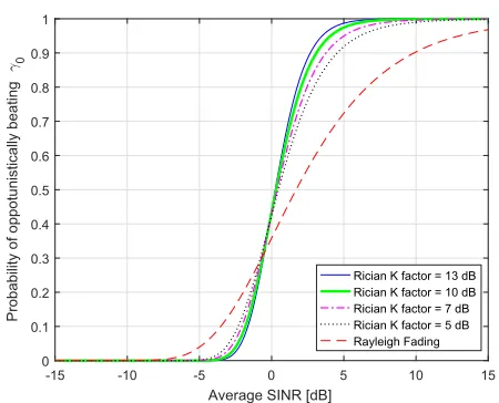
To corroborate the above result, Fig.2compares the proba-bility that the coverage probaproba-bility opportunistically beats the SINR threshold of γ0 = 0dB for both Rician fading with
different Rician K factors as well as Rayleigh fading. Note that the Rician K factors of 13, 10, 7, and 5 dB correspond to 3D distances of 0 m, 100 m, 200 m, and 266.6 m between UE and BS, respectively. This has to be emphasized that as discussed in Section II, the distance-dependent Rician fading model with a variant RicianKfactor adjusts the dominance of the LOS path based on distance between UE and BS. It can be seen that when the BS density is low, which corresponds to the high SINR regime (3 dB ∼ 10 dB), Rician fading has a better chance to satisfy the SINR threshold requirement in comparison to Rayleigh fading, which leads to a better coverage probability performance. However, in the low SINR regime (-10 dB ∼ -3 dB), which corresponds to a high BS density, and thus UD-SCN, the RicianKfactor is larger (LOS fading dominates) and hence the Rician fading has a lower chance to reach the SINR threshold requirement in comparison to Rayleigh fading. As a result, it can be expected that Rician fading more sharply drags down both the coverage probability and ASE performance to zero than Rayleigh fading.
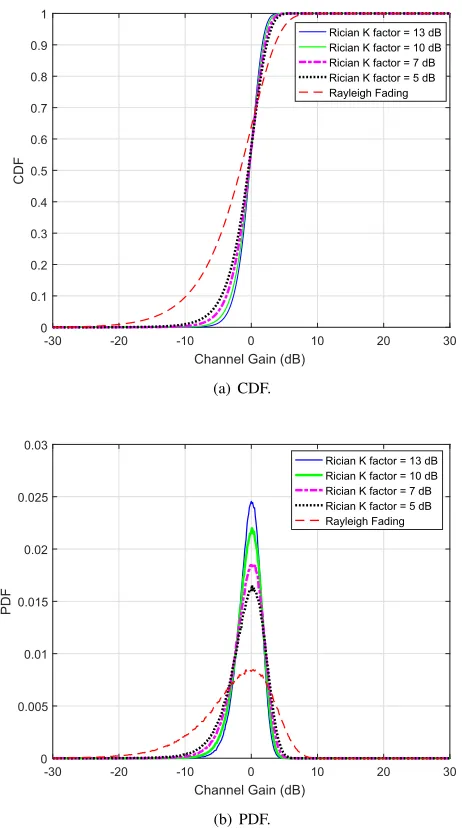
To support the above discussion, Fig. 3compares the CDF and PDF of Rician fading with different Rician K factors to that of Rayleigh fading. It is seen that while Rayleigh fading has a larger variance around the mean, Rician fading has a more deterministic behaviour due to dominant LOS component with a smaller variance around its mean. The higher the density of BSs in the network, the larger the Rician K factor, the stronger the LOS component, and the smaller the variance.
C. Study of a 3GPP Special Case
We consider the following 3GPP path loss function used in [27]
ζ(w) =
(
ALw−αL,
ANLw−αNL,
with probability PrL(w)
with probability 1−PrL(w) ,
(13)
-30 -20 -10 0 10 20 30
ChanneltGaint(dB) 0
0.1 0.2 0.3 0.4 0.5 0.6 0.7 0.8 0.9 1
CDF
RiciantKtfactort=t13tdB RiciantKtfactort=t10tdB RiciantKtfactort=t7tdB RiciantKtfactort=t5tdB RayleightFading
(a) CDF.
-30 -20 -10 0 10 20 30
Channel7Gain7(dB) 0
0.005 0.01 0.015 0.02 0.025 0.03
Rician7K7factor7=7137dB Rician7K7factor7=7107dB Rician7K7factor7=777dB Rician7K7factor7=757dB Rayleigh7Fading
[image:5.612.319.550.58.472.2](b) PDF.
Fig. 3. Comparison of CDF and PDF of Rician and Rayleigh fadings.
which for sake of simplicity and without any loss of generality uses a linear LOS probability [28] function, PrL(w), defined as
PrL(w) =
(
1− w d1,
0,
0< w≤d1
w > d1
, (14)
where the steepness of PrL(r)is defined by the parameterd1.
According to Theorem 1 and considering the mentioned 3GPP case, Pcov(λ, γ) can be computed as Pcov(λ, γ) =
2
P
n=1
TL
n+TnNL
, where ζL
1(w) = ζ2L(w) = ALw−α
L
,
ζ1NL(w) = ζ2NL(w) = ANLw−αNL, PrL1(w) = 1− w d1, and
PrL2(w) = 0. In the following, we computeTL
1, which can then
be easily extended to{TP ath
we derive the lower bound of was
wLB=
w≥L tight when r is very small, i.e.,0≤r≤v1
w≥ r√+L
2 tight when r is relatively small, i.e.,
v1≤r≤v2
w≥r tight when r is relatively large, i.e.,r > v2.
(15) wherev1=
p
(2)−1Landv2=
p
(2) + 1L. Having computed the lower bound, we approximate was L, r√+L
2and
r for the ranges ofrdiscussed in (15), respectively.
According to Theorem 1 and based on the above approx-imation, TL
1 for the range of 0 < r ≤
p d2
1−L2 can be
computed as
T1L =
ˆ √d2 1−L2
0
∞ X
k=0
k X
m=0
J(m, k)γk−m(−1)k−m
∂k−mLL
Ir(
γ Ptζn(L
√
r2+L2))
∂γk−m f
L
R,1(r)dr (16)
where ζL
1(w) = ALw−α
L
and LL
Ir refers to the Laplace
transform ofIratsfor the LOS transmission. Moreover, from Theorem 1, fL
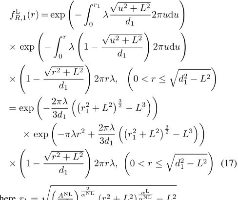
R,1(r)can be obtained as
fR,L1(r) = exp −
ˆ r1
0
λ
√
u2+L2
d1
2πudu !
×exp −
ˆ r
0
λ 1−
√
u2+L2
d1
!
2πudu !
× 1− √
r2+L2
d1
!
2πrλ,
0< r≤qd2
1−L2
= exp
−2πλ
3d1
r21+L232−L3
×exp
−πλr2+2πλ 3d1
r21+L232 −L3
× 1− √
r2+L2
d1
!
2πrλ,
0< r≤qd2
1−L2
(17)
wherer1=
r
ANL
AL
αNL2
(r2+L2)ααNLL −L2.
Breaking the integration interval into different segments, we calculate the definite integrals Q1 =
´b
a(1 −∆1)udu
and Q2 =
´b
a(1 − ∆2)u √
u2+L2du where ∆1 = (eKsPtApath)−1(
√
u2+L2)αpath
1+(sPtApath)−1(
√
u2+L2)αpath−K(sP
tApath)−1(
√
u2+L2)αpath and
∆2=
(eKsPtApath)−1(
√
u2+L2)αpath
1+(sPtApath)−1(
√
u2+L2)αpath−K(sP
tApath)−1(
√
u2+L2)αpath
for different segments of [0≤ a;b ≤v1], [v1 ≤ a;b ≤v2],
[v2≤a;b <∞], and [v2 ≤a;b= +∞] which are presented
in Appendix B.
IV. SIMULATION ANDDISCUSSION
In this section, we use numerical results to study the performance of dense SCNs with non-identical antenna heights
10-2 100 102 104
BSadensitya [1/km2]
0 0.1 0.2 0.3 0.4 0.5 0.6 0.7 0.8 0.9 1
CoverageaProbability
[image:6.612.324.571.56.246.2] [image:6.612.63.300.216.279.2]RicianaRicianaAAnalytical) RicianaRayleighaAAnalytical) RayleighaRicianaAAnalytical) RayleighaRayleighaAAnalytical) RicianaRicianaASimulation) RicianaRayleighaASimulation) RayleighaRicianaASimulation) RayleighaRayleighaASimulation)
Fig. 4. The coverage probability versus BS density with antenna height difference of L = 10m.
under Rician fading channel and validate the accuracy of our analysis. To analyse in detail the impact of the Rician Crash theorem in UD-SCNs, we consider four different cases:
• Case 1: Both serving and interfering BSs are subject to Rician fading,
• Case 2: Serving BS is subject to Rician fading, while
interfering BSs are subject to Rayleigh fading,
• Case 3: Serving BS is subject to Rayleigh fading, while
interfering BSs are subject to Rician fading,
• Case 4: Both serving and interfering BSs are subject to Rayleigh fading.
Note that case 1 is more realistic and that the other cases are presented here in order to aid the discussion. Also note that in the legend of Figs.4and5, the first and second terms refer to the channel model between the UE and its serving and interfering BSs, respectively.
We adopt the following parameters in our numerical analysis based on [27], [29]. We assume the LOS and NLOS path loss exponents of αL = 2.09 and αNL = 3.75. Moreover, AL,
ANL, and d
1 are assumed to be 10−10.38, 10−14.54, and 0.3
km, respectively. The transmit and noise power are also equal to Pt = 24 dBm and N0 = −95 dBm. Unless mentioned
otherwise, we also assume antenna height differences ofL= 0
(identical UE and BS antenna heights) andL= 8.5m.
A. The Coverage Probability Performance
Fig.4shows the coverage probability versus the BS density for the four cases discussed above, where the UE and BS antennas are not at the same height (L= 8.5m). First of all and before proceeding with the analysis of numerical results, it is important to note that the theoretical analysis results match the simulation results, and thus we only discuss theoretical results hereafter.
[image:6.612.57.301.338.543.2]probability initially increases with the BS density, as the network is light up with coverage. However, once the BS density exceeds a certain threshold, in this case λ0= 20kmBss2
, the difference between the heights of UE and BS antennas causes a cap on the signal power, which prompts the coverage probability to decline and eventually converge to zero, as was explained in Rician Crash Theorem. Comparing the coverage probability of the four different cases presented above, it can be seen that the multi-path fading model (as discussed in Lemma 1) does have an impact on the coverage probability, when there is a difference in the heights of the UE and the BS antennas.
When the coverage probability achieves its maximum at
λ1, meaning that the UE SINRs are large, the case with
Rician fading for the serving links and Rayleigh fading for the interference links achieves the best performance. This is in line with Lemma 1, which showed that Rician fading has a better chance to satisfy the SINR threshold requirement in comparison to Rayleigh fading in the high SINR regime between 3 dB and 10 dB. To further support this claim note that, as it was shown in Fig.3, Rician fading results in a more deterministic multi-path fading due to its specular dominant LOS component with a lower variance around the mean, while Rayleigh fading has a larger variance around the mean with a large tail towards the negative values, resulting in fadings of up to -20dB, The first phenomena helps to maintain a good carrier signal for most UEs, while the second one helps to opportunistically mitigate the interference.
When the coverage probability is low, which refers to low SINR regime, it is important to note that there is a cross over at around λ1= 700kmBss2
between the coverage probabilities of the cases that have Rician and Rayleigh fading to model the serving links. This is also in line with Lemma1, which showed that Rician fading has a lower chance to reach the SINR threshold requirement in comparison to Rayleigh fading in the low SINR regime between−3 dB and−10dB. The cases with Rayleigh fading offer a better performance here because Rayleigh fading benefits from more channel fluctuations than Rician fading, and thus achieves an opportunistic carrier signal power gain, which is only visible at low UE SINRs. In such regime, the case with Rayleigh fading for both the serving and the interference links achieves the best performance, since as explained before the Rayleigh interference is in average smaller than the Rician one.
B. The ASE Performance
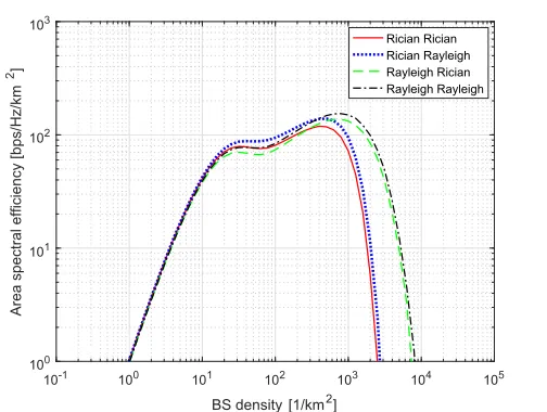
Fig.5shows the ASE performance for the above four differ-ent cases. It is important to mdiffer-ention that we only focus on the theoretical results and so the ASE results are obtained from the coverage probability presented in (7). The ASE performance also follows a similar trend as the coverage probability. For all the four cases, we can see that as far as the BS density is lower than λ1, the ASE linearly increases with the BS
density because the coverage holes are mitigated. Densifying the network beyondλ1causes the ASE to experience a slower
growth pace or even a decrease. This occurs due to coverage
10-1 100 101 102 103 104 105
BSzdensityz [1/km2]
100 101 102 103
Areazspectralzefficiencyz[bps/Hz/km
2]
RicianzRician RicianzRayleigh RayleighzRician RayleighzRayleigh
Fig. 5. The area spectral efficiency versus BS density with antenna height difference of L = 10m.
probability degradation triggered by the transition of a large number of interfering signals from NLOS to LOS [18], [23]. Then, when the BS density is large, as in an UD-SCN, we observe a severe degradation in ASE performance due the UE and BS antenna height difference, and that such degradation greatly depends on the multi-path fading model.
Comparing the ASE results that correspond to the discussed four cases, we can also realise the same behaviour as for the coverage probability. When the BS density isλ1 and the
coverage probability achieves its maximum, the cases with Rician fading at the serving links provide the best performance because Rician fading has a better chance to meet the SINR threshold. However, when the UE SINR starts to degrade due to the difference between UE and BS antenna heights, the cases with Rayleigh fading are more robust and provide a better performance since Rayleigh fading benefits from a higher chance to meet the SINR threshold, as was derived in Lemma 1 and shown in Fig. 2. Accordingly, when the multi-path channel between the UE and its associated BS is Rician fading, the ASE declines more rapidly towards zero. As network becomes denser and the LOS component becomes more dominant, the RicianK factor is reinforced causing the Rician fading to face a more severe exponential decay. To further explain this, we must note that due to the large Rician
K factor in UD-SCN (where the channel is even prone to single LOS tap), Rician fading causes less fluctuations in the channel in comparison to Rayleigh fading, which prevents to benefit from the opportunistic channel gains. Rayleigh fading instead provides such opportunistic SINR gains at the cell-edge, which leads to an enhanced ASE. As a result, the Rician fading causes a more severe performance degradation as discussed by Rician Crash theorem.
[image:7.612.320.572.55.245.2]10-1 100 101 102 103 104 105 BSHdensityH[1/km2]
10-1
100 101 102 103
104 105 106
AreaHspectralHefficiencyH[bps/Hz/km
2]
[image:8.612.60.290.59.244.2]RicianHFadingH)LH=H0) RicianHFadingH)LH 0)
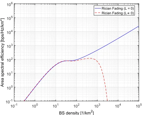
Fig. 6. Comparison of the area spectral efficiency with different antenna heights under Rician fading.
and BS have same antenna heights (L= 0), the ASE linearly increases as the network moves towards an UD-SCN [23]. In contrary, based on the Rician Crash theorem, when (L6= 0), Rician fading causes the ASE to severely drop to zero. This suggests that operators should lower the small cell BS height close to the average UE antenna height when deploying UD-SCNs.
C. Discussion on the Value of Theoretical Analysis
While theoretical derivations do not have straightforward and compact expressions, this has to be pointed out that computer based simulations are nearly infeasible when looking at a practical ultra-dense network with a tremendous number of BSs, millions of them. The complexity of computer based simulations quickly become prohibitive, with running times of around a month for the discussed scenario in this paper. In more details, the required time to perform the computer based simulations for BS densities ofλ≥103BSs/km2is very long,
and it becomes almost infeasible for BS densities of λ≥105
BSs/km2. For instance, for BS density ofλ= 106BSs/km2, it
takes a minimum of twenty seven days to plot smooth curves using computer based simulations in comparison to five days using the theoretical derivations. In contrast, the complexity of the theoretical analysis remains independent of the BS density, thanks to the numerical integration derived in this paper, i.e., the complexity is not a function of the BS density and so the results can be obtained much faster.
V. CONCLUSION
In this paper, we analysed the impact of Rician fading on the coverage probability and ASE performance in UD-SCNs where the BS and UE antennas are not of the same height. Using a piecewise path loss model, we showed through analytical expressions as well as simulation results that due to less channel fluctuations of Rician fading, it causes the ASE to more rapidly slope down to zero in comparison to Rayleigh fading. This indicates that multi-path fading plays a key role
in UD-SCNs with non-identical UE-BS antenna heights and to avert its ruinous effect, the operators should deploy small cell BSs close to the height of the average UE antenna.
ACKNOWLEDGEMENT
The work is partially sponsored by H2020 ”is3DMIMO” project.
REFERENCES
[1] CISCO, “Cisco visual networking index: Global mobile data traffic forecast update (2013-2018),” Feb. 2014.
[2] ArrayComm and William Webb, Ofcom, London, U.K., 2007. [3] D. L´opez-P´erez, M. Ding, H. Claussen, and A. H. Jafari, “Towards
1 Gbps/UE in cellular systems: understanding ultra-dense small cell deployments,” IEEE Commun. Surveys and Tutorials, vol. 17, no. 4, pp. 2078-2101, Fourthquarter 2015.
[4] J. Ling, D. Chizhik, “Capacity scaling of indoor pico-cellular networks via reuse”, IEEE Commun. Letters, vol. 16, no. 2, pp. 231-233, Feb. 2012.
[5] H. Holma and A. Toskala,LTE for UMTS – OFDMA and SC-FDMA
Based Radio Access, John Wiley & Sons Ltd., 2009.
[6] A. H. Jafari, D. L´opez-P´erez, H. Song, H. Claussen, L. Ho, and J. Zhang, “Small Cell Backhaul: Challenges and Prospective Solutions,”EURASIP
J. on Wireless Commun. and Netw., vol. 2015, no. 1, pp. 1-18, 2015.
[7] H. Zhang, Y. Dong, J. Cheng, M. J. Hossain and V. C. M. Leung, “Fronthauling for 5G LTE-U Ultra Dense Cloud Small Cell Networks,”
IEEE Wireless Commun. Mag., vol. 23, no. 6, pp. 48-53, Dec. 2016.
[8] A. H. Jafari, V. Venkateswaran, D. L´opez-P´erez, and J. Zhang,“Diversity Pulse Shaped Transmission in Ultra-Dense Small Cell Networks,”IEEE
Trans. Veh. Technol., vol. 66, no. 7, pp. 5866-5878, Jul. 2017.
[9] A. H. Jafari, V. Venkateswaran, D. L´opez-P´erez, and J. Zhang,“Pulse shaping diversity to enhance throughput in ultra-dense small cell net-works,”Proc. of IEEE SPAWC, Jul. 2016.
[10] H. Zhang, S. Huang, C. Jiang, K. Long, V. C. M. Leung and H. V. Poor,“Energy Efficient User Association and Power Allocation in Millimeter-Wave-Based Ultra Dense Networks With Energy Harvesting Base Stations,”IEEE J. Sel. Areas Commun., vol. 35, no. 9, pp. 1936-1947, Sep. 2017.
[11] Z. Zhang, H. Zhang, Z. Zhao, H. Liu, X. Wen and W. Jing,“Low com-plexity energy-efficient resource allocation in down-link dense femtocell networks,”Proc. of IEEE PIMRC, Sep. 2013.
[12] Nokia, ”Ultra Dense Network (UDN),” 2016.
[13] Z. Zhang, H. Zhang, Z. Lu, Z. Zhao and X. Wen,“Energy-efficient resource optimization in OFDMA-based dense femtocell networks,”
Proc. of IEEE ICT, Apr. 2013.
[14] W. Ma, H. Zhang, W. Zheng and X. Wen,“Differentiated-pricing based power allocation in dense femtocell networks,”Proc. of IEEE WPMC, Sep. 2012.
[15] J. G. Andrews, F. Baccelli, and R. K. Ganti, “A tractable approach to coverage and rate in cellular networks,”IEEE Trans. on Commun., vol. 59, no. 11, pp. 3122-3134, Nov. 2011.
[16] H. S. Dhillon, R. Ganti, F. Baccelli, and J. G. Andrews, “Modeling and analysis of K-tier downlink heterogeneous cellular networks,”IEEE J.
Sel. Areas Commun., vol. 30, no. 3, pp. 550-560, Apr. 2012.
[17] S. Singh, H. S. Dhillon, and J. G. Andrews, “Offloading in heterogeneous networks: modeling, analysis, and design insights,” IEEE Trans. on
Wireless Commun., vol. 12, no. 5, pp. 2484-2497, May 2013.
[18] M. Ding, P. Wang, D. L´opez-P´erez, M. Ding, G. Mao and Z. Lin, “Performance Impact of LoS and NLoS Transmissions in Dense Cellular Networks,”IEEE Trans. on Commun., vol. 15, no. 3, pp. 2365-2380, Mar. 2016.
[19] M. Ding, D. L´opez-P´erez, G. Mao, P. Wang and Z. Lin, “Will the area spectral efficiency monotonically grow as small cells go dense?,”Proc.
of IEEE Globecom, Dec. 2015.
[20] X. Zhang, J. G. Andrews, “Downlink cellular network analysis with multi-slope path loss models,”IEEE Trans. on Commun., vol. 63, no. 5, pp. 1881-1894, Mar. 2015.
[22] T. Bai, R. W. Heath Jr., “Coverage and rate analysis for millimeter wave cellular networks,”IEEE Trans. on Wireless Commun., vol. 14, no. 2, pp. 1100-1114, Oct. 2014.
[23] A. H. Jafari, M. Ding, L´opez-P´erez, and J. Zhang “On the Performance Impact of Rician Fading on Dense Networks with LOS/NLOS Trans-missions,”submitted to IEEE Wireless Commun. Lett., Mar. 2017. [24] M. Ding, D. L´opez-P´erez, “Performance Impact of Antenna Heights
in Dense Cellular Networks,” submitted to IEEE Trans. on Wireless
Commun., 2016.
[25] M. Haenggi, Stochastic Geometry for Wireless Networks. Cambridge University Press, 2012.
[26] C. Galiotto, N. K. Pratas, N. Marchetti, L. Doyle, “A stochastic geometry framework for LOS/NLOS propagation in dense small cell networks”, [Online]. Available: http://arxiv.org/abs/1412.5065
[27] 3GPP, “TR 36.828 (V11.0.0): Further enhancements to LTE Time Division Duplex (TDD) for Downlink-Uplink (DL-UL) interference management and traffic adaptation,” Jun. 2012.
[28] Spatial Channel Model AHG, “Subsection 3.5.3, Spatial Channel Model Text Description V6.0,” Apr. 2003. ([Online]: ftp://www.3gpp.org/tsg ran/WG1 RL1/3GPP 3GPP2 SCM/ConfCall-16-20030417)
[29] 3GPP, “TR 36.872, Small cell enhancements for UTRA and E-UTRAN - Physical layer aspects,” Dec. 2013.
[30] A. H. Jafari, D. L´opez-P´erez, M. Ding, and J. Zhang, “Study on Scheduling Techniques for Ultra Dense Small Cell Networks, ”Proc.
of IEEE VTC, Sep. 2015.
[31] 3GPP, “TR 25.996, Spatial channel model for Multiple Input Multiple Output (MIMO) simulations,” Sep. 2012.
[32] Y. Li and J. Li and J. Jiang and M. Peng, “Performance analysis of device-to-device underlay communication in Rician fading chan-nels,”Proc. of IEEE Globecom, Dec. 2013.
[33] M. Peng and Y. Li and T. Q. S. Quek and C. Wang, “Device-to-Device Underlaid Cellular Networks under Rician Fading Channels,”
IEEE Trans. on Wireless Commun., vol. 13, no. 8, pp. 4247-4259, Aug.
2014.
[34] I.S. Gradshteyn and I.M. Ryzhik,Table of Integrals, Series, and Products
(7th Ed.), Academic Press, 2007.
[35] R. L. Burden and J. D. Faires, Numerical Analysis (3rd Ed.), PWS Publishers, 1985.
APPENDIXA
To compute Pcov(λ, γ), we need to calculate two
parame-ters: i) the joint distance PDFs for the corresponding events of the typical UE being associated with a BS with either a LOS or NLOS path represented by Events BL
n andBnNL, respectively, and ii) the coverage probability that is conditioned on r, BL
n
and r, BNL
n
. Note that the joint distance PDF ofrand Event
Bpath
n with string variable pathtaking the values of{L,NL} to represent LOS and NLOS paths is denoted by fR,npath(r), wherefR,npath(r) is subject to the following condition:
N X
n=1
ˆ √d2
n−L2
√ d2
n−1−L2
fR,nL (r)dr+
N X
n=1
ˆ √d2
n−L2
√ d2
n−1−L2
fR,nNL(r)dr= 1.
(18) Also note that the coverage probability is the sum of the probabilities associated with the Events BL
n andBnNL, owing to the fact that these two events are disjoint.
To computefR,nL (r), we refer to its definition asfR,nL (r) =
fR,n|BL
n r|B L
n
Pr[BL
n], where Pr[BnL] = Pr
L
n( √
r2+L2)
andfR,n|BL
n r|B L
n
represents the joint event that corresponds to the following independent sub-events.
• The serving BS b0 should be located at a 2D distancer
from the typical UE with the corresponding unconditional distance PDF of 2πrλ.
• There should not be any other LOS BS than the serving
BSb0 in eventBnL that offers a better link to the UE. Its probability is given as
pLn(r) = exp
−
ˆ r
0
PrLpu2+L22πuλdu
.
(19)
• There should not be any other NLOS BS than the serving
BSb0 in eventBnL that offers a better link to the UE. Its probability is given as
pNLn (r) = exp
−
ˆ r1
0
1−PrLpu2+L22πuλdu
,
(20)
where r1 = arg
r1
n
ζNLp
r2 1+L2
=ζL
n √
r2+L2o
to derive the 2D distance at which the NLOS BS andb0
offer the same signal level.
Assuming a 3D distance, we can show that
fR,n|BL
n r|B L
n
=pNLn (r)pLn(r)2πrλ. (21)
Therefore, the piecewise PDF of the distance to the LOS and NLOS serving BS can be derived as
fR,nL (r) = exp
−
ˆ r1
0
1−PrLpu2+L22πuλdu
×exp
−
ˆ r
0
PrLpu2+L22πuλdu
PrLnpr2+L2
×2πuλ,
q
d2n−1−L2< r≤p d2
n−L2
, (22)
and
fR,nNL (r) = exp
−
ˆ r2
0
PrLpu2+L22πuλdu
×exp
−
ˆ r
0
1−PrLpu2+L22πuλdu
×1−PrLnpr2+L2×2πuλ,
q
d2
n−1−L2< r≤
p d2
n−L2
, (23)
where r1 = arg
r1
n
ζNLp
r2 1+L2
=ζL
n √
r2+L2o
and
r2= arg
r2
ζLpr22+L2=ζNL
n √
r2+L2 .
We can now move on to evaluate PrSINR> γ| r, BL
n
and Pr
SINR> γ| r, BNL
n
, which can be presented as Pr
Ptζn(L
√
r2+L2)h
Ir > γ
and Pr
PtζnNL(
√
r2+L2)h
Ir > γ
, respectively. In the following, we only consider
Pr[Ptζ
L
n(√r2+L2)h
Ir > γ], as Pr[
PtζnNL(
√
r2+L2)h
can be computed in the same manner.
Pr[Ptζ L
n √
r2+L2
h Ir
> γ]
=E[Ir]
(
Pr
"
h > γIr
PtζnL √
r2+L2
# )
=E[Ir]
(
¯
FH
γIr
PtζnL √
r2+L2
! )
(24)
where E[Ir]{.} is the expectation operation over the random
variableIrandF¯H(h)refers to the complementary cumulative distribution function (CCDF) of random variable h. Note that for the tractability of analysis, we have considered an interference-limited scenario in our derivations. Moreover, the interference is normalized with respect to PtζnL
√
r2+L2
, where the normalized interference is defined as Irn =
Ir
Ptζn(L
√
r2+L2). Therefore, (24) can be expressed asPr[
h Irn >
γ] = 1 −Pr[Ih
rn < γ] where Pr[
h
Irn < γ] denotes the
cumulative distribution function (CDF) of the normalized SINR, and thusPr[Ih
rn < γ]can be written as
Pr[ h
Irn
> γ] = 1−
ˆ ˆ
h y<γ
fH(h)fIrn(y) dhdy
= 1−
ˆ ∞
0
FH(γy)fIrn(y) dy (25)
where fH(h) and FH(h) are the PDF and CDF of random variable h, respectively [32], [33]. Since the random variable
his Rician distributed, its PDF is given by
fH(h) =
(K+ 1) ¯
h exp
−
K+(K+ 1)¯ h
h
× I0(
r
4K(K+ 1)h
¯
h ) (26)
where K is the Rician K factor, I0 is the zero-th order
first kind modified Bessel function and ¯h is expectation of
h. Applying the series expansion from [34], [35],fH(h)can be expressed as fH(h) = exp(−K−h)
∞ P
k=0 (Kh)k
(k!)2 and using
the PDF ofh, its CDF can be derived as
Fh(h) = exp(−K)
∞ X
k=0
Kk
(k!)2 exp(−h)
k X
m=0
(−1)2m+1 m!
k
m
hk−m+k!
!
=−
∞ X
k=0
k X
m=0
exp(−h)J(m, k)hk−m +
∞ X
k=0
Kk
k! exp(−K)
=−
∞ X
k=0
k X
m=0
exp(−h)J(m, k)hk−m+ 1 (27)
where J(m, k) = exp(−K)K km!(k
m) (k!)2 and
∞ P
k=0
Kk
k! = exp(K)
based on the Taylor series combination. By replacing (27) in
(25), we derive
Pr[ h
Irn
> γ] =
∞ X
k=0
k X
m=0
J(m, k)
ˆ ∞
0
(yγ)k−me−yγfIrn(y) dy
=
∞ X
k=0
k X
m=0
J(m, k)γk−mQ(γ, k−m) (28)
where Q(τ, n) = ´0∞yne−yτfIrn(y)dy = (−1)
n ∂nLIrn(τ)
∂τn
for n= 0,1, ..,∞[32], [33]. Therefore,
Pr[ h
Irn
> γ] =
∞ X
k=0
k X
m=0
J(m, k)γk−m(−1)k−m
∂k−mLILrn(γ)
∂γk−m (29)
PluggingIr=Irn PtζnL √
r2+L2
into (29), we can derive
Pr[Ptζ L
n √
r2+L2
h Ir
> γ] =
∞ X
k=0
k X
m=0
J(m, k)γk−m
(−1)k−m
∂k−mLL
Ir(
γ Ptζn(L
√
r2+L2))
∂γk−m (30)
whereLL
Ir(s)is the Laplace transform of RV Irevaluated at
s subject to the condition corresponding to Event BL which
states that the UE is associated with a BS with LOS trans-mission. Similarly, for the NLOS transmission, it is derived as
Pr
" PtζnNL
√
r2+L2
h Ir
> γ #
=
∞ X
k=0
k X
m=0
J(m, k)γk−m
(−1)k−m
∂k−mLNL
Ir (
γ PtζnNL(
√
r2+L2))
∂γk−m (31)
whereLNL
Ir (s) is the Laplace transform of RVIr evaluated
atssubject to the condition corresponding to EventBNL that
the UE is associated with a BS with NLOS transmission. In the following, we deriveLL
Ir(s)as
LL
Ir(s) =E[Ir]
exp (−sIr)|BL
=E[Φ,{βi},{gi}]
exp
−s
X
i∈Φ/bo
Ptβi(w)gi
BL
(32)
and based on the path loss model, the user is subject to interference from both LOS and NLOS paths. Therefore,
Therefore,LL
Ir(s)can be expressed as
LL
Ir(s) = exp −2πλ
ˆ ∞
r
1− √
u2+L2
d1
!
1−E[g]exp
−sPtAL p
u2+L2−α
L
g
udu !
×exp −2πλ
ˆ ∞
r1
√
u2+L2
d1
1−E[g]exp
−sPtANL
p
u2+L2−
αNL
g
udu !
(33)
For sake of presentation, the term sPtAL √
u2+L2−αL
is denoted by Λ, and thusE[g]{exp(−Λg)}can be computed as
E[g]exp(−Λg) =
ˆ ∞
0
exp(−Λg) exp(−K−g)
∞ X
k=0 (Kg)k
(k!)2 dg (34)
where exp(−K −g)
∞ P
k=0 (Kg)k
(k!)2 is the PDF of the random
variable g. According to Taylor series, it is realized that
∞ P
k=0
Kk
k! = exp(K), and thus (34) can be written as E[g]{exp(−Λg)}=
ˆ ∞
0
exp(−Λg)exp(−K−g)exp(Kg) dg
= exp(−K)
ˆ ∞
0
exp(−g(1 + Λ−K)) dg= exp(−K) 1 + Λ−K(35)
Plugging Λ = sPtAL √
u2+L2−αL
into (35), 1 −
E[g]exp(−sPtAL √
u2+L2−αL
g)can be written as
1−E[g]exp(−sPtAL p
u2+L2−α
L
g) =
1−(e KsP
tAL)−1 √
u2+L2αL
1 + Γ1 (36)
where Γ1 = (sPtAL)−1 √
u2+L2αL
− K(sPtAL)−1 √
u2+L2αL
. Similarly, 1−E[g]{exp(−sPtANLu−α
NL
g)}
can be computed, and thus (33) is written as
LL
Ir(s) = exp −2πλ
ˆ ∞
r
1− √
u2+L2
d1
!
1−
(eKsPtAL)−1 √
u2+L2αL
1 + Γ1
udu
!
×exp −2πλ
ˆ ∞
r1
√
u2+L2
d1
1−
(eKsP
tANL)−1 √
u2+L2αNL
1 + Γ2
udu
!
(37)
where Γ2 = (sPtANL)−1 √
u2+L2αNL
−K(sPtANL)−1 √
u2+L2αNL
and s= γ(
√
r2+L2)αL
PtAL . By plugging (37) in
(30), we compute Pr[PtζLn(
√
r2+L2)h
Ir > γ]. In a similar
man-ner, we can deriveLINL
r (s), and obtainPr[
PtζNLn (
√
r2+L2)h
Ir >
γ]and, therefore,
Pr[Ptζ L
n √
r2+L2
h Ir
> γ] =
∞ X
k=0
k X
m=0
J(m, k)γk−m
(−1)k−m
∂k−mLILr
γ PtζLn(
√
r2+L2)
∂γk−m (38)
and
Pr[Ptζ NL
n √
r2+L2
h Ir
> γ] =
∞ X
k=0
k X
m=0
J(m, k) γk−m
(−1)k−m
∂k−mLNL
Ir
γ PtζnNL(
√
r2+L2)
∂γk−m (39)
where LL
Ir(s) and L NL
Ir (s) refer to the Laplace transform
of RV Ir evaluated at s for LOS and NLOS transmissions, respectively, and are derived as
LL
Ir(s) = exp −2πλ
ˆ ∞
r
1− √
u2+L2
d1
!
1−(e KsP
tAL)−1 √
u2+L2αL
1 + Γ1
!
udu !
×exp −2πλ
ˆ ∞
r1
√
u2+L2
d1
1−(e KsP
tANL)−1 √
u2+L2αNL
1 + Γ2
!
udu !
and
LNL
Ir (s) = exp −2πλ
ˆ ∞
r2
1− √
u2+L2
d1
!
1−(e KsP
tAL)−1 √
u2+L2αL
1 + Γ1
!
udu !
×exp −2πλ
ˆ ∞
r √
u2+L2
d1
1−(e KsP
tANL)−1 √
u2+L2αNL
1 + Γ2
!
udu !
. (41)
APPENDIXB
In the following, we calculate the the definite integrals Q1
andQ2 for the different segments.
Case 1: Assuming 0 ≤ a andb ≤v1, we approximate
√
u2+L2≈L. Therefore, Q
1andQ2can be expressed
as
Q1 ≈
ˆ b
a
1−
(eKsP
tApath)−1Lα
path
1 + (sPtApath)−1Lα
path
−K(sPtApath)−1Lα
path
Ludu=1
2 b 2−a2
+a 2−b2
2 (eKsPtApath)−1Lα
path
1 + (sPtApath)−1Lαpath−K(sPtApath)−1Lαpath (42)
and
Q2 ≈
ˆ b
a
1−
(eKsPtApath)−1Lα
path
1 + (sPtApath)−1Lαpath−K(sPtApath)−1Lαpath
udu= L
2 b 2−a2
+L a 2−b2
2 (eKsP
tApath)−1Lα
path
1 + (sPtApath)−1Lα
path
−K(sPtApath)−1Lα
path (43)
Case 2: Assuming v1 ≤ a and b ≤ v2, we
approxi-mate √u2+L2 ≈ u√+L
2 . Therefore, Q1 andQ2 can be
expressed as
Q1 ≈
ˆ b
a
1−
(eKsP
tApath)−1
u√+L
2
αpath
1 + (sPtApath)−1
u√+L
2
αpath
−K(sPtApath)−1
u√+L
2
αpath
udu ˆ b+L
a+L
1−
(eKsP
tApath)−1
¯
u
√
2
αpath
1 + (sPtApath)−1
¯
u
√
2
αpath
−K(sPtApath)−1
¯
u
√
2
αpath
(¯u−L)d¯u
=ρ1
αpath,1,
(sP
tApath)−1 √
2 (1−K)
, b+L
−ρ1
αpath,1,
(sP
tApath)−1 √
2 (1−K)
, a+L
−L "
ρ1
αpath,0,
(sP
tApath)−1 √
2 (1−K)
, b+L
−ρ1
αpath,0,
(sPtApath)−1 √
2 (1−K)
, a+L
#
+(sPtApath)−1 (1−K−exp(−K))
1
√
2
αpath!
× "
ρ1
αpath, αpath+ 1,
(sPtApath)−1 √
2 (1−K)
, b+L
−ρ1
αpath, αpath+ 1,
(sP
tApath)−1 √
2 (1−K)
, a+L
#
+L(sPtApath)−1(1−K−exp(−K)) ×
"
ρ1
αpath, αpath,
(sP
tApath)−1 √
2 (1−K)
, b+L
−ρ1
αpath, αpath,
(sP
tApath)−1 √
2 (1−K)
, a+L
#
(44)
and
Q2 ≈
ˆ b
a
1−
(eKsP
tApath)−1
u√+L
2
αpath
1 + (sPtApath)−1
u√+L
2
αpath
−K(sPtApath)−1
u√+L
2
αpath
uu√+L
=
ˆ b+L
a+L
1−
(eKsPtApath)−1
¯
u
√
2
αpath
1 + (sPtApath)−1
¯
u
√
2
αpath
−K(sPtApath)−1
¯
u
√
2
αpath
(¯u−L)¯u
√
2 d¯u =√1
2
ρ1
αpath,2,
(sPtApath)−1 √
2 (1−K)
, b+L
−ρ1
αpath,2,
(sP
tApath)−1 √
2 (1−K)
, a+L
− √L
2
"
ρ1
αpath,1,
(sP
tApath)−1 √
2 (1−K)
, b+L
−ρ1
αpath,1,
(sP
tApath)−1 √
2 (1−K)
, a+L
#
+ (sPtApath)−1
(1−K−exp(−K))
√
2
1
√
2
αpath
× "
ρ1
αpath, αpath+ 2,
(sP
tApath)−1 √
2 (1−K)
, b+L
−ρ1
αpath, αpath+ 2,
(sP
tApath)−1 √
2 (1−K)
, a+L
#
+L(sPtA
path)−1(1−K−exp(−K))
√
2
× "
ρ1
αpath, αpath+ 1,
(sP
tApath)−1 √
2 (1−K)
,
b+L
− ρ1
αpath, αpath+ 1,
(sP
tApath)−1 √
2 (1−K)
,
a+L
#
(45)
where the variable change of u+L= ¯uis used to ease the integrations. Note thatρ2(α, β, t, d)is defined as
ρ1(α, β, t, d) =
ˆ d
0
uβ
1 +tuαdu
=
dβ+1
β+ 1
2F1
1,β+ 1 α ; 1 +
β+ 1
α ;−td
α
(46)
where2F1[., .;.;.]refers to the hyper-geometric function.
Case 3: Assumingv2≤aandb <∞, we approximate
√
u2+L2≈u. Therefore,Q
1andQ2 can be expressed
as
Q1 ≈
ˆ b
a
1−
(eKsPtApath)−1uα
path
1 + (sPtApath)−1uαpath−K(sPtApath)−1uαpath
udu
=ρ1 αpath,1,(sPtApath)−1(1−K), b −ρ1 αpath,1,(sPtApath)−1(1−K), a
+ (1−K−exp(−K))
ρ1 αpath,1,(sPtApath)−1
(1−K), b
−ρ1 αpath, αpath+ 1,(sPtApath)−1
(1−K), a
(47)
and
Q2 ≈
ˆ b
a
1−
(eKsP
tApath)−1uα
path
1 + (sPtApath)−1uαpath−K(sPtApath)−1uαpath
u2du
=ρ1 αpath,2,(sPtApath)−1(1−K), b
−ρ1 αpath,2,(sPtApath)−1(1−K), a
+ (1−K−exp(−K))
ρ1 αpath, αpath+ 2, (sPtApath)−1(1−K), b
−ρ1 αpath, αpath+ 2, (sPtApath)−1(1−K), a
(48)
Case 4:Assumingv2≤aandb= +∞, we approximate
Q1 andQ2 as
Q1 ≈
ˆ +∞
a
1−
(eKsPtApath)−1uα
path
1 + (sPtApath)−1uαpath−K(sPtApath)−1uαpath
udu
=ρ2 αpath,1,(sPtApath)−1(1−K), a
+ (sPtApath)−1(1−K−exp(−K))
×ρ2 αpath, αpath+ 1,(sPtApath)−1(1−K), a
(49)
and
Q2 ≈
ˆ +∞
a
1−
(eKsP
tApath)−1uα
path
1 + (sPtApath)−1uαpath−K(sPtApath)−1uαpath
u2du
=ρ2 αpath,2,(sPtApath)−1(1−K), a
+ (sPtApath)−1(1−K−exp(−K))
×ρ2 αpath, αpath+ 2,(sPtApath)−1(1−K), a
(50)
whereρ2(α, β, t, d)is defined as
ρ2(α, β, t, d) =
ˆ ∞
d
uβ
1 +tuαdu
=
d−(α−β−1)
t(α−β−1)
2F1
1,1−β+ 1
α ; 2−
β+ 1
α ;−
1
tdα
.
(51)