Automated shark detection using computer vision

(1)

University of Southern Queensland

Faculty of Health, Engineering & Sciences

Automated Shark Detection using Computer Vision

A dissertation submitted by

K. Byles

in fulfilment of the requirements of

ENG4112 Research Project

towards the degree of

(2)

Abstract

With the technological advancements of UAVs, researchers are finding more ways to

har-ness their capabilities to reduce expenses in everyday society. Machine vision is at the

forefront of this research and in particular image recognition. Training a machine to

iden-tify objects and di↵erentiate them from others plays an integral role in the advancement

of artificial intelligence. This project aims to design an algorithm capable of automatically

detecting sharks from a UAV. Testing is performed by post-processing aerial footage of

sharks taken from helicopters and drones, and analysing the reliability of the algorithm.

Initially this research project involved analysing aerial photography of sharks, dissecting

the images into the individual colour channels that made up the RGB and HSV colour

spaces and identifying methods to detect the shark blobs. Once an adaptive threshold

of the brightness channel was designed, filters were curated specific to the environments

presented in the obtained aerial footage to reject false positives. These methods were

considerably successful in both rejecting false positives and consistently detecting the

sharks in the video feed.

The methods produced in this dissertation leave room for future work in the shark

detec-tion field. By acquiring more reliable data, improvements such as using a kalman filter to

detect and track moving blobs could be implemented to produce a robust shark detection

(3)

University of Southern Queensland Faculty of Health, Engineering & Sciences

ENG4111/2 Research Project

Limitations of Use

The Council of the University of Southern Queensland, its Faculty of Health, Engineering

& Sciences, and the sta↵ of the University of Southern Queensland, do not accept any

responsibility for the truth, accuracy or completeness of material contained within or

associated with this dissertation.

Persons using all or any part of this material do so at their own risk, and not at the risk of

the Council of the University of Southern Queensland, its Faculty of Health, Engineering

& Sciences or the sta↵of the University of Southern Queensland.

This dissertation reports an educational exercise and has no purpose or validity beyond

this exercise. The sole purpose of the course pair entitled “Research Project” is to

con-tribute to the overall education within the student’s chosen degree program. This

doc-ument, the associated hardware, software, drawings, and other material set out in the

associated appendices should not be used for any other purpose: if they are so used, it is

entirely at the risk of the user.

Dean

(4)

Certification of Dissertation

I certify that the ideas, designs and experimental work, results, analyses and conclusions

set out in this dissertation are entirely my own e↵ort, except where otherwise indicated

and acknowledged.

I further certify that the work is original and has not been previously submitted for

assessment in any other course or institution, except where specifically stated.

K. Byles

(5)

Acknowledgments

I would like to thank my friends and family for providing positive criticism on my work

throughout the duration of this project. Dr Tobias Low was always able to o↵er

construc-tive feedback, and didn’t leave me feeling abandoned or lost in any way.

Most of all I’d like to acknowledge my loving girlfriend Katherine, for I would not be

where I am today without her undoubted support.

(6)

List of Figures

1.1 Diagram of shark net. . . 2

1.2 Diagram of shark drumline. . . 2

1.3 Shark seen o↵Boudlers beach near Ballina from a helicopter. . . 3

1.4 A great white shark tagged with both acoustic (front) and pop-up satellite (rear) tags. The acoustic tag is detected when the shark swims within 250m of a listening station, while the pop-up satellite tag records information about location, temperature and depth - and relays it to the laboratory when the tag releases itself from the shark. . . 3

1.5 Example of di↵erent colour channels compiled together. . . 5

1.6 An example of the RGB colour space. . . 6

1.7 An example of the HSV colour space. . . 7

1.8 An example of the LAB colour space. . . 7

1.9 An example of image processing being used to enhance the beauty of a model. . . 8

1.10 Illustration of finding the local maxima for an edge . . . 10

(11)

LIST OF FIGURES x

1.12 Illustration of detected edge points within the predetermined thresholds.

As shown, edges remain consistent within the low to high boundary if they

are connected to edge points that eventually go above the high threshold

level. The line below the low threshold represents noise in the data. . . . 11

1.13 Image of figurine imported into Matlab and converted to grayscale. . . 11

1.14 Canny edge detection applied to the figurine and edges dilated. . . 11

1.15 Original image of cell. . . 12

1.16 Edge detection applied to image. . . 12

1.17 Edges dilated with ’imdilate’ function in Matlab. . . 12

1.18 Images filled with ’imfill’ function. . . 12

1.19 Images connected to border are removed. . . 13

1.20 Blobs not connected to the main blob are ’eroded’. . . 13

1.21 The perimeter of the segmented image is overlayed on the original image. 13 2.1 Results of dugong detection study illustrating 7 out of 13 dugongs detected, no false positives. . . 19

2.2 Layers of CNN used to detect dugongs. . . 19

2.3 Blob analysis using a CNN filtering out blobs based on confidence scores. 20 2.4 Blobs detected after edge detection, coral blackening and blob filling. . . . 20

2.5 Success rate of vision system. . . 21

2.6 Frame divided into di↵erent areas and histogram bin thresholding applied. 21 2.7 E↵ects of GMM and background subtraction. . . 22

2.8 Frame showing snake detection. . . 22

2.9 Frame showing jellyfish detection. . . 22

(12)

LIST OF FIGURES xi

2.11 Sample frame of traffic. . . 24

2.12 Background subtraction and blob analysis performed to identify white cars. 24 3.1 Screenshot from drone footage of shark in coastal waters . . . 27

3.2 Screenshot from drone footage of shark in coastal waters . . . 27

3.3 Risk Assessment Matrix. . . 32

4.1 Test image. . . 34

4.2 RGB representation of current test image. The red, green and blue data arrays are saved to individual variables and displayed as a surface model. This will help identify methods for pixel thresholding. . . 35

4.3 HSV representation of current test image. The hue, saturation and value data arrays are saved to individual variables and displayed as a surface model. This will help identify methods for pixel thresholding. . . 36

4.4 Frames used to test the relationship of lower pixel values for identified sharks in the Red, Green and Value arrays. . . 37

4.5 3D surface model for Red, Green and Value arrays for test image 1 at side and aerial views. . . 38

(13)

LIST OF FIGURES xii

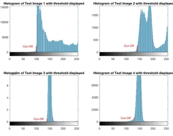
4.10 Histograms of Test Images displaying cut-o↵ threshold. Most populated

bins represent pixels related to the water. Everything to the right of the

cut-o↵is ignored. . . 45

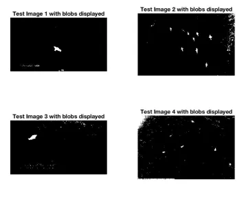
5.1 Binary maps of test images after thresholding. No morphology performed yet. . . 47

5.2 How a computer ’sees’ a shark. . . 47

5.3 Binary map of shark. . . 47

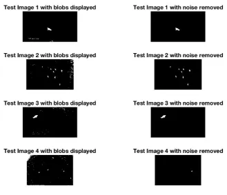
5.4 Binary maps of test images before and after morphology to remove noise. 48 5.5 Morphology applied to frame with a surfer in the field of view. . . 49

5.6 Morphology applied to frame with a surfer in the field of view. . . 50

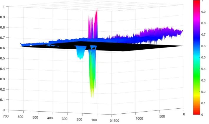
5.7 3D surface model depicting dark patches of water being falsely detected. . 51

5.8 Original Image and stages in filtering out unwanted regions of interest. . . 52

5.9 Histogram of Elliptic Ratios of Blob Database. . . 53

6.1 Frame 33: Shark detected in frame. . . 57

6.2 3D surface model of frame 33. . . 57

6.3 Frame 84: False negative. . . 57

6.5 Frame 369: Two sharks detected in frame. . . 58

6.7 Frame 498: Missed detection of two sharks. . . 59

6.9 Frame 595: One true positive, One false negative and One true negative. . 60

(14)

LIST OF FIGURES xiii

6.13 Frame 883 False negative. . . 61

6.15 Frame 1545: Shark successfully detected. . . 62

(15)

LIST OF FIGURES xiv

6.37 Frame 433: Whitewash rejects shark detection. . . 69

6.41 Frame 885: Area of shark too small for detection. . . 71

6.45 Frame 3663: False positive. . . 72

6.47 Frame 5000: Brightness ratio rejects shark. . . 73

(16)

List of Tables

3.1 Project Resource Requirements . . . 30

6.1 Frame 33: Values of blob elements . . . 57

(17)

LIST OF TABLES xvi

(18)

List of Algorithms

1 Display Surf Models of Pixel Densities . . . 34

2 Display Blob Outlines on Original Image . . . 42

3 Calculate Threshold for Regions of Interest . . . 44

4 Region of Interest Filtering . . . 50

5 Remove Dark Patches of Water . . . 52

(19)

Chapter 1

Introduction

1.1

Background

Shark attacks have haunted every swimmer at some point in their life. The ominous

shadows of the deep lurking below them, the object that brushed past their feet or the

cool chill of something not being right has often reminded people of the horror of being a

big fish’s lunch. In the last 100 years in Australia alone there have been 543 unprovoked

shark attacks, with 135 of those people losing their lives (Taronga 2016). Although for a

statistician those aren’t overwhelming odds, the long-term trend indicates an increasing

number of shark attacks which is most likely due to an increasing number of people

swimming at the beach. To try and reduce the frequency of shark attacks there have

been a few control methods put in place such as:

• Shark nets

– These are used to entangle sharks and prevent them from reaching swimmers

and surfers. The nets are typically placed 500 metres o↵shore and are 150m

wide and 6m tall (Sealifetrust 2015) and submerged in water of depths around

10m. Shark nets have been known to kill marine life such as dolphins and

(20)

1.1 Background 2

Figure 1.1: Diagram of shark net.

• Drumline

– Consists of baited hooks that are set in waters 6m to 12m deep and

approx-imately 600m o↵shore (Sumpton et al. 2011). The hooks are checked and

re-baited every 15-20 days by contracted fisherman, who thoroughly record

each catch.

Figure 1.2: Diagram of shark drumline.

• Aerial Patrol

– These have been used to monitor the beaches from small planes and helicopters.

A recent study in 2014 recorded the success rate of identifying artificial shark

analogues placed at an average 2.5m below the surface of the ocean was 12.5%

for fixed-wing and 17.1% for helicopters (Robbins, Peddemors, Kennelly &

Ives 2014). A typical aerial patrol can involve a sweep of nearly 300km of

coastline, where the plane or helicopter is only o↵ering a couple minutes of

(21)

1.1 Background 3

Figure 1.3: Shark seen o↵Boudlers beach near Ballina from a helicopter.

• Tagging

– Sharks are tagged and monitored over a certain time period, where the data

obtained is typically used to determine migration patterns. Other useful data

can be the depth at what the shark dives to for a given time period and

the temperature of the water (Holmes, Pepperell, Griffiths, Jaine, Tibbetts &

Bennett 2014). Tagged sharks can o↵er real-time tracking (News.com.au 2015)

but it is not feasible to track down every shark and install a tag on them.

Figure 1.4: A great white shark tagged with both acoustic (front) and pop-up satellite (rear) tags. The acoustic tag is detected when the shark swims within 250m of a listening station, while the popup satellite tag records information about location, temperature and depth -and relays it to the laboratory when the tag releases itself from the shark.

• Spotters

– Professional spotters that scan the water from a high point such as a cli↵ or

(22)

1.2 Computer Vision 4

In light of these expensive control methods in place, shark attacks are still occurring. To

combat this the author is proposing a shark detection system based on aerial photography,

which could greatly reduce funding needed for shark control methods and o↵er real-time

surveillance and alerts of sharks in dangerous or threatening positions.

1.2

Computer Vision

Computer vision is a broad topic that involves many areas and is apart of everyday life.

Medical professionals use computer vision for x-rays and MRI’s to better diagnose their

patients. Architects and engineers use computer vision for 3D modelling. Toll points

and parking lots use computer vision to recognise license plates on vehicles. Production

plants use computer vision for automatic inspection of goods on assembly lines to check

for imperfections, and the list goes on. As science and engineering progress, computer

vision is establishing a greater impact on society.

Computer vision can be a very complex area, and in the words of Richard Szeliski, ”despite

all advances in computer vision, the dream of having a computer interpret an image at the

same level as a two-year old (for example, counting all the animals in a picture) remains

elusive”. This is because vision is an inverse problem (Szeliski 2010), in which we seek

to recover some unknowns given insufficient information to fully specify the problem. We

must therefore resort to physics-based models and probabilistic models to disambiguate

between potential solutions.

Computers interpret images as arrays of numbers and cannot be taught to identify objects

by what shape they are. Instead di↵erent mathematical techniques are used to determine

how the relative pixel of varying densities are arranged to each other. An edge might be

detected by a sharp sudden change in pixel density, whilst a shape may be detected by

an arrangement of such edges in a circular, mathematical fashion.

Dr Adrian Rosebrock, author of Practical Python and OpenCV, defines a pixel as ”a

colour or the intensity of light that appears in a given place in an image”. Digital cameras

are quite often ranked for their resolution, or by how many pixels are in the photos that

the camera produces. The resolution is the product of the rows of pixels multiplied by the

columns, because images are digitally stored as arrays of pixel intensities that represent

(23)

1.3 Colour Spaces 5

ranked from 0 to 255 with 0 being no colour at all (black) and 255 being the maximum

(white). In RGB (colour) images there are three layers of arrays, each relating to the 3

di↵erent colour channels red, green and blue. Every pixel in the arrays are given a value

of intensity (or how much of that colour the pixel is trying to represent) out of 0 to 255.

For example, a bluish almost purple might have pixel values of 200 for blue, 100 for red

and 50 for green.

Figure 1.5: Example of di↵erent colour channels compiled together.

1.3

Colour Spaces

A colour space or model is a way to mathematically represent the formulation of colours

from the combination of primary colours. Additive colour models are primarily designed

for electronic systems such as televisions, computers and digital photography. There are

3 dominant models that are typically used in computer vision.

(24)

1.3 Colour Spaces 6

of 3 primary colours, red, green and blue. In order to create a colour with RGB, three

light coloured beams (red, green and blue) must be superimposed (Insights 2016). With

no intensity, each of the 3 colours is perceived as black, while full intensity is perceived

as white. Varying the intensities varies the output colour.

Figure 1.6: An example of the RGB colour space.

HSV (hue, saturation and value) colour space depicts 3D colour. HSV seeks to describe

relationships between colours, and improve on the RGB colour model. HSV can be

illustrated as a wheel where the centre axis goes from white at the top to black at the

bottom, with other neutral colours in between. The angle from the axis represents the

hue, the distance from the axis depicts the saturation, and the distance along the axis

(25)

1.3 Colour Spaces 7

Figure 1.7: An example of the HSV colour space.

LAB colourspace is designed to approximate human vision. Unlike RGB, LAB is not

device-dependant. In this 3D model, the ’L’ stands for the lightness of the colour, with 0

producing black and 100 producing a di↵used white. The ’A’ is the redness vs. greenness

and the ’B; is the yellowness vs. blueness (Insights 2016).

(26)

1.4 Image Processing 8

1.4

Image Processing

Image processing involves editing and manipulating digital images to enhance its visual

e↵ects or to make it more user-friendly for complex computer vision applications. A

common use of image processing is in advertising or media, where models can be digitally

enhanced to improve their attractiveness or for products to seem more appealing. Image

processing is typically the first step in a computer vision algorithm, where features can be

transformed, enhanced, blurred and more to make the image more user-friendly for the

algorithm to process. For example, a colour recognition algorithm might begin with an

image being blurred so that insufficient details are removed, making the probability of a

blob of a certain predetermined colour being detected higher. Filters used for smartphone

applications such as ’Snapchat’ and ’Instagram’ are good examples of image processing

as they enhance or warp images when applied.

Figure 1.9: An example of image processing being used to enhance the beauty of a model.

1.5

Edge Detection

Edge detection is a process which involves the computer automatically highlighting all

the edges in the image through a series of operations. These operations typically involve

filtering, di↵erentiation and detection. One of the most successful and commonly used

edge detectors is the Canny edge detector, developed by John F. Canny in 1986. Canny

had specified performance criteria for the detector to meet (Shah 1997) such as:

1. Good Detection. The optimal detector must minimise the probability of false

posi-tives as well as false negaposi-tives.

(27)

1.5 Edge Detection 9

edges

3. Single Response Constraint. The detector must return one point only for each edge

point.

The reason for this criteria was to help minimise unwanted noise that was apparent in

other detectors such as the Marr-Hildreth detector where the Laplacian of the Gaussian

was used to locate zero crossings which indicated an edge. The steps in the Canny edge

detector are:

1. Smooth image with Gaussian filter g(x, y)

g(x, y) = p1

2⇡ e

x2+y2

2 2 (1.1)

S=I⇤g(x, y) (1.2)

2. Compute derivative of filtered image

rS =_r(g_⇤I) = gx gy

⇤I (1.3)

3. Find magnitude and orientation of gradient

(Sx, Sy) Gradient Vector

magnitude =q(S2

x+Sy2)

direction = ✓= tan 1 Sy

Sx

4. Apply ”non-maximum suppression”

The pixels that are perpendicular to the identified edge must be suppressed so that

thick edges are minimised. This is done by locating a point (x, y) and determining

(28)

Figure 1.10: Illustration of finding the local maxima for an edge

M(x, y) = 8 > > > > > < > > > > > :

|rS_|(x, y) if _|_rS_|(x, y)>_|_rS_|(x0, y0)

& |rS|(x, y)>|rS|(x00, y00)

0 otherwise

(1.4)

5. Apply ”hysteresis threshold”

If the gradient at a pixel is

-above ’high’, declare it as an edge pixel

-below ’low’, declare it as a non-edge pixel

-between ’low’ and ’high’, consider its neighbours iteratively then declare it an edge

pixel if it is connected to an edge pixel directly or via pixels between ’low’ and

’high’.

(29)

Scan the image from left to right, top to bottom. If the gradient magnitude at the

pixel is above the high threshold, declare that as an edge point. Then recursively

look at its neighbours. If the gradient magnitude is above the low threshold, declare

that as an edge point.

Figure 1.12: Illustration of detected edge points within the predetermined thresholds. As shown, edges remain consistent within the low to high boundary if they are connected to edge points that eventually go above the high threshold level. The line below the low threshold represents noise in the data.

Edge detection is quite often used as the first step in blob detection, where the

outlines of objects are detected. Further image processing techniques involving

dilation, fill and erosion help to isolate the object. An example of edge detection

can be seen in Figure 1.14 where canny edge detection has been applied to a photo of

a figurine holding a computer. The edges were then dilated for illustration purposes.

Figure 1.13: Image of figurine imported into Matlab and converted to grayscale.

(30)

1.6 Image segmentation 12

1.6

Image segmentation

Image segmentation has been widely applied in image analysis for various areas such

as biomedical imaging, intelligent transportation systems and satellite imaging (Choong,

Kow, Chin, Angeline, Tze & Teo 2012). The main goal of image segmentation is to cluster

pixels into salient image regions, i.e. regions corresponding to individual surfaces, objects

or natural parts of objects (Bodhe 2013). After regions are successfully segmented into

individual regions they can then be identified automatically as seen in pest detection

systems for horticulture (Bodhe 2013).

Mathworks have o↵ered several examples that explain the basics of image segmentation.

Detecting a shark in the water, which in theory should be a controlled environment

depending on the amount of light available, could be formulated using edge detection and

basic morphology. The example as published by Mathworks (Mathworks 2016h) for cell

detection could prove to be a good starting point in developing a algorithm for identifying

sharks. The example works in six steps:

Figure 1.15: Original image of cell. Figure 1.16: Edge detection applied to im-age.

Figure 1.17: Edges dilated with ’imdilate’ function in Matlab.

(31)

1.7 Object Tracking 13

Figure 1.19: Images connected to border are removed.

Figure 1.20: Blobs not connected to the main blob are ’eroded’.

Figure 1.21: The perimeter of the seg-mented image is overlayed on the original image.

This is a very good example of how the blob of the shark might be obtained. Further

analysis could determine whether the blob is of a ’shark’ size by identifying how many

pixels make up the blob. Although the depth of image is unknown, if an assumed operating

height of the drone is known then relative blob sizes can be calculated.

1.7

Object Tracking

Object tracking involves the detection of objects and tracking their movement over

mul-tiple frames. It is typically used in surveillance type systems and can be broken down

into 3 main steps:

• Object detection

(32)

• Object tracking

1.7.1 Object Detection

Object detection is the process of finding instances of real-world objects such as faces,

bicycles and buildings in images or videos (Mathworks 2016i). Object detection is still

very limited in everyday use in society as it is extremely difficult for a computer to

automatically detect objects, as explained earlier, a computer can only define an object

by the arrangement and intensities of the pixels in the image. However, face detection

and people tracking systems are becoming more popular and plenty of research is being

undertaken to develop more complex surveillance systems.

To locate a moving object in consecutive video frames the following 3 methods can be

applied:

• Frame Di↵erencing

– Frame di↵erencing works by checking the di↵erence between 2 consecutive

frames. It employs the input as 2 image frames of video and produces the

output as the di↵erence of the pixel values. This is obtained by subtracting

pixel values of the second frame from the first frame (Kothiya 2015). As a

result, moving objects can be easily detected in videos with static backgrounds.

• Optical Flow

– Optical flow is a technique that presents an apparent change in the moving

object’s location between consecutive frames of the video (Kothiya 2015). It

employs the motion field that represents the direction and velocity of each

point in every frame. It is a computationally expensive method that is more

suitable for multiple moving object detection.

• Background Subtraction

– The background subtraction method involves removing the background so that

only the foreground moving objects are left. Consecutive images are compared

to find the di↵erence in pixel values so that moving objects can be identified.

This method is ideal for static backgrounds and can deal with multiple moving

(33)

1.7.2 Object Classification

Once a moving object has been detected it must be classified to identify what the object

is. The following methods are typically used for object classification:

• Shape based classification

– The shape information of a moving object can be retrieved from the

repre-sentation of the blob. It can then be compared through matching techniques

using complex SIFT or SURF features, or by testing for a certain size or shape.

Matching techniques generally require a large database with thousands of test

images, both positive and negative to compare against.

• Motion based classification

– This involves analysing the velocity of the pixels related to an object and

classifying them with respect to their known speed. Such applications could

involve traffic cameras detecting cars travelling faster than the speed limit.

• Colour based classification

– Objects can easily be identified that are of a known consistent colour. This

method works best when the object of interest is a considerably di↵erent colour

to the background.

• Texture based classification

– Texture can be used as a feature by identifying the variation in pixel intensities

for a given region of interest. Texture classification involves learning and

recog-nition. Learning consists of identifying the texture features for a given object

and recognition attempts to match the texture features with the subsequent

frames.

1.7.3 Object Tracking

The typical methods of object tracking are:

(34)

– Point based tracking is a complex problem as it can result in false detections

and the occlusion of objects in frames (Kothiya 2015). The various methods

of point based tracking are:

∗ Kalman filter

· The Kalman filter is based on the probability density function. It is a relatively complex method that is designed to return the optimal

solution.

∗ Particle filter

· Particle filtering generates all models for one state variable before it moves to the next state variable. The trajectory of the tracked object

can be determined by taking the particle with the highest weight of

the particle set at each time step (Hess 2009).

∗ Multiple hypothesis tracking

· This process is also known as an iterative algorithm that begins with a set of existing track hypothesis (Kothiya 2015). The object’s position

in every frame is made for each hypothesis. Cham and Rehg’s (Cham

& Rehg 1999) study of tracking people dancing demonstrates that this

method is capable of handling occlusion and can track multiple objects.

• Kernel based tracking

– Kernel based tracking relates to the appearance of an objects shape. The

kernel can be elliptical or rectangular and is able to track objects in translation

and rotation. Simple template matching, mean shift method, support vector

matching and layered based matching are all examples of kernel based tracking

(Kothiya 2015).

• Silhouette based tracking

– Silhouette based tracking involves using the information encoded inside an

object region for tracking. This is ideal for objects that have complex shapes

such as shoulders, fingers and hands that cannot be described adequately by

simple geometric shapes. Silhouette tracking is typically achieved by contour

(35)

1.8 Project Aim 17

1.8

Project Aim

This dissertation aims to research object classification by means of computer vision and

determine whether an automated shark detection system can be established. The

ap-proach taken to design the shark detection algorithm will be from an aerial perspective,

with the end goal being an Unmanned Aerial Vehicle (UAV) patrolling the coastal waters

and alerting a control station or lifeguards if a shark is detected.

On the 29th of February 2016, the NSW premier Mike Baird unveiled a$250,000 military

grade shark-spotting drone called the ”Little Ripper” (Chang 2016) which states that it

uses real-time sensor and pattern recognition algorithms. Although it is still in the testing

phase, the drone is said to be able to identify sharks better than the naked eye.

The proposal of drones policing the coastal waters for sharks o↵ers an inexpensive early

shark detection method in comparison to having helicopter and fixed-wing surveillance.

If the shark detection algorithm can be taught to identify sharks with minimal error, such

as false positives or missing targets, it may pave the way for a foolproof shark surveillance

system that eradicates the need for expensive piloted aerial patrols.

1.9

Research Objectives

For the system to be feasible, it needs to show that it can identify sharks and have minimal

false positives. To reach this state, the following research objectives must be met:

• Carry out a literature review that is relevant to image segmentation, object recog-nition, object classification and object tracking.

• Obtain aerial videos of sharks in coastal waters to begin designing the algorithm with.

• Write a basic computer vision program that can detect the ’blob’.

• Expand on the basic blob detection algorithm by trying to filter out all of the blobs that aren’t relative to a shark.

(36)

Chapter 2

Literature Review

The areas that have been researched for this project are computer vision and techniques

relevant to object classification, object recognition and tracking.

2.1

Segmentation methods of marine wildlife from UAV’s

Recent studies have proved limited success in detecting wildlife from UAV’s. In 2013

a study was conducted by students from QUT (Queensland University of Technology)

titled ’Detection of Dugongs from Unmanned Aerial Vehicles’ (Maire, Mejias, Hodgson &

Duclos 2013). The dugongs were segmented by identifying them by colour thresholding

and determining the red-ratio of pixels. To limit false positives ’whitecaps’ were identified

and ’inpainted’ to reduce the confusion of similar shaped bright pixels. The whitecaps

were detected by identifying a relationship between the mean of the colour channel ’c’ in

the image and determining whether the a pixel was greater than that scaled mean.

To further classify the dugongs and limit false positives, a binary map was made of the

detected blob and overlayed on a template to determine the similarity. It was discovered

that a blob was more likely to relate to a dugong if its shape was elliptical, so by extracting

information such as the ’MajorAxisLength’ and ’MinorAxisLength’ of the detected blob

and calculating its elliptical area, it could be compared to the area of the blob template.

The closer to 1 this relationship was the higher the probability of the detected blob being

a dugong.

(37)

2.1 Segmentation methods of marine wildlife from UAV’s 19

conditions as ever-changing waves and reflections would result in a lot of false positives.

Figure 2.1: Results of dugong detection study illustrating 7 out of 13 dugongs detected, no false positives.

2.1.1 Dugongs and Machine Learning

Machine learning has been another method researchers have investigated to perform

au-tomatic analysis of aerial video footage. CNNs (Convolutional Neural Networks) have

been the key component in pattern recognition systems, and are predominantly used in

face detection and OCR (Optical Character Recognition) systems. Research from the

University of Queensland investigated whether a CNN could be used to apply automatic

detection to dugongs (Maire, Mejias & Hodgson 2014). By compiling two LeNet

convo-lutional layers, a hidden layer and then a logistic regression layer, (Maire et al. 2014) was

able to predict whether there were any dugongs in a given frame.

Figure 2.2: Layers of CNN used to detect dugongs.

The success rate of the CNN was found to be feasible, but was limited to lower resolution

images as the classifier had been trained on 28 x 28 input windows due to a small training

set. It was concluded that it was difficult to compare to methods previously used because

the bounding boxes of dugongs were typically 100 x 100 (Maire et al. 2013). A larger

(38)

2.2 Underwater Fish Detection 20

window.

Figure 2.3: Blob analysis using a CNN filtering out blobs based on confidence scores.

2.2

Underwater Fish Detection

The estimation of fish population and species classification has been an interesting

ap-plication of blob analysis (Fabic, Turla, Capacillo, David & Naval 2013). The study,

conducted by the University of the Philippines, utilised an underwater camera to capture

local schools of fish inhabiting coral. The basis of this study was to determine a method

using computer vision to count and determine the species of fish. Such information would

be helpful to marine biologists to track and monitor fish species and their habitats.

Figure 2.4: Blobs detected after edge detection, coral blackening and blob filling.

The algorithm first used histogram comparison to identify coral and ’blacken’ it out. Once

the coral had been removed, edge detection was applied to the frame to identify contours

related to fish. These contours were then filled to represent ’blobs’, and then filtered and

categorised by size. This allowed the vision system to di↵erentiate between the two fish

species within the frame, the parrot fish and the sturgeon fish. The system proved to be

(39)

2.3 Marine object detection 21

Figure 2.5: Success rate of vision system.

2.3

Marine object detection

Other algorithms, such as jellyfish and sea snake detection, use what is known as a hybrid

detection method to correctly identify objects of interest (Zhou, Llewellyn, Wei, Creighton

& Nahavandi 2015). This hybrid method is composed of statistical learning techniques,

such as Gaussian mixture modelling, and feature based approaches.

One of the main problems with dealing with marine object detection is being able to

remove all the pixels related to the water, and just leave the objects of interest. To achieve

this in the jellyfish and snake detection, a Gaussian mixture model which could be trained

automatically to recognise background pixels (water) (Zhou et al. 2015). Automatic

collection of training pixels was segregated into di↵erent areas of the training frame, due

to the lighting distribution. Histogram models were made of each area of the frame, and

bin thresholding was applied to determine which pixels were related to the background.

Figure 2.6: Frame divided into di↵erent areas and histogram bin thresholding applied.

(40)

2.3 Marine object detection 22

K clusters using the Orchard-Bouman algorithm (Orchard & Bouman 1991). Image

seg-mentation is then applied to di↵erentiate between the foreground and background groups,

based on the Otsu algorithm (Yu, Dian-ren, Yang & Lei 2010). Standard morphology

op-erations such as fill holes, eroding and dilating help remove any noise and leave the blobs

of the sea life defined.

Figure 2.7: E↵ects of GMM and background subtraction.

Blob analysis was then performed to classify the snakes and jellyfish. Blob selection

cri-teria such as blob height to width ratio, area to bounding box ratio and circularity (using

Heywood’s circularity factor) allowed the snakes and jellyfish to be correctly classified.

The disclosed results determined a detection rate of over 90% over a sample size of 243

images (frames with snakes or jellyfish in them) collected over two years.

Figure 2.8: Frame showing snake detection.

Figure 2.9: Frame showing jellyfish detection.

2.3.1 LiDAR Detection and Classification of Subsurface Objects

LiDAR detection systems have also been investigated for marine object detection (Cianciotto

1997), due to their resilience to weather conditions as opposed to traditional computer

vision techniques. Airborne LiDAR systems have been used for research in:

• Detection of submerged objects

• Oil spill detection and identification

(41)

2.4 Blob Analysis 23

• Atmospheric pollution surveillance

• Stratospheric dust measurements

• Subsurface ocean temperature measurements

The advantages of these LiDAR systems is that LiDAR is typically able to see objects

3-5 times deeper than conventional computer vision systems, which would be ideal for

locating sharks that are too submerged for a camera to identify. LiDAR systems are

however quite expensive, leaving this possible avenue unavailable for the author.

2.4

Blob Analysis

Blob analysis has also been widely used in vehicle counting, pedestrian tracking and traffic

sign recognition. By identifying what makes an image unique, pixel thresholding can be

performed to remove pixels that are unrelated to the region of interest. This can involve

manipulating colour spaces such as RGB, HSV and LAB. Research from the University

of Ostrava demonstrated pixel thresholding in the HSV colour space when attempting to

detect and classify traffic signs (Zavadil & Tuma 2012). By ’ANDing’ pixel conditions

for all three channels (hue, saturation and value), he was successful in identifying the

pixels most likely related to the traffic signs. From there, analysis of the blob properties

was performed to determine the geometry of the blob, and the Mahalanobis distance

was computed to determine the similarity score against a reference set of images. The

testing was performed on a robot race track, and images were captured within 2m of the

upcoming traffic symbol. Of the 321 positive frames, only 15 false negatives were obtained

and 0 false positives. The following graph illustrates the results:

(42)

2.5 Project Area of Research 24

Vehicle counting is another good demonstration of blob analysis, where background

sub-traction is utilised to remove all stationary pixels. Therefore stationary cameras can be

set up at busy intersections, and be programmed to count each car (blob) that is moving.

This is a much more e↵ective way to record traffic flow information than to have people

continually noting down the cars driving past. Research from the GMR Institute of

Tech-nology, India, illustrated how background subtraction can be utilised, and blob analysis

can be performed to allow the vision system to identify light coloured cars driving past

(Telagarapu 2012).

Figure 2.11: Sample frame of traf-fic.

Figure 2.12: Background subtrac-tion and blob analysis performed to identify white cars.

Background subtraction has also been widely used in people detection and counting

systems. Research from the Pozna University of Technology demonstrated that

peo-ple entering a building could be identified, counted and tracked, by removing the

back-ground and applying blob analysis to the detected moving pixels (Tchn, Kfnqhsglr, Mc,

Shnmr, Marciniak, D¸abrowski, Chmielewska, Nowakowski, Wkh, Ri, Lq, Uhvhdufk &

Uhvxowlqj 2012) . Although background subtraction can be a useful tool in elementary

object detection solutions, it is certainly not feasible for a shark detection system where

the waves are constantly moving and changing.

2.5

Project Area of Research

Based on the findings of the literature review this project will be focused on determining

an appropriate pixel thresholding method to identify the shark blobs within the frame

(43)

2.5 Project Area of Research 25

These methods will involve converting the image to alternate colour spaces for analysis

(Zavadil & Tuma 2012), applying pixel thresholding techniques and determining blob

at-tributes such as elliptic ratio (Maire et al. 2013), and investigating other unique properties

of the shark blobs to enable the shark detection algorithm to filter out false positives with

(44)

Chapter 3

Methodology

This chapter discusses the approach that will be taken to design, develop and evaluate

the shark detection algorithm on its feasibility.

3.1

Project Methodology

Computer vision can be an elusive task that is prone to error, and unfortunately the

solution to one object detection problem can not simply be applied to another. That is

why the methodology for this project will involve many alterations. The development

stage of the algorithm will involve countless changes and tweaking to first, attempt to

isolate the shark from the image and then optimise the isolation and tracking process.

To further discuss the methodology of the project, the project has been segregated into

tasks:

1. Determine the tools required such as software packages and electronics

2. Obtain useful videos of sharks in coastal waters

3. Determine trends in pixel variations and colour spaces

4. Develop an adaptive thresholding method for identifying regions of interest

5. Morphological operations

(45)

3.2 Task Analysis 27

7. Develop tracking methods

8. Determine feasibility and highlight why the algorithm is successful or not

3.2

Task Analysis

The following sections highlight the key components of the designated tasks.

3.2.1 Determine the tools required such as software packages and elec-tronics

The programming environment for the development of the shark detection algorithm

has been chosen to be MATLAB. This software o↵ers some very useful computer vision

and image processing functions and its matrix representation makes it incredibly easy to

analyse images. The MATLAB suite combined with the computer vision toolbox is $155.

All other necessary equipment such as a laptop with Microsoft office are already owned

by the author.

3.2.2 Obtain useful videos of sharks in coastal waters

The author has already reached out to sharkspotting groups on facebook and marine

biologists but has been unable to acquire any aerial videos of sharks. However, there are

some videos on youtube that may be suitable for image processing. The following images

are snapshots from two of the videos:

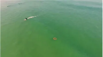
Figure 3.1: Screenshot from drone footage of shark in coastal waters

(46)

Videos where the drone is ’sweeping’ the coast may prove difficult to work with, so only

necessary snippets of the videos where the drone is hovering above a shark will be used.

3.2.3 Determine trends in pixel variations and colour spaces

The first step of the algorithm will be blob analysis. Colour thresholding can be performed

to remove unwanted objects in an image such as removing dark objects such as roads and

converting the resulting image to a binary map (Telagarapu & Suresh 2012). To identify

what colour thresholds to implement to localise the sharks, RGB and HSV colour channels

will analysed to determine reliable trends in the pixel representation of the sharks. If a

reliable trend can be identified, a threshold will be applied that sets all pixels outside the

desired range of the pixel to zero. The result of this will be transformed into a binary

map which shows the blobs of interest.

3.2.4 Develop an adaptive thresholding method for identifying regions of interest

The problem with computer vision in an uncontrolled environment is how sensitive the

system can become due to changes in illumination. To actively set a threshold to locate

the regions of interest, a relationship will have to be determined between lighting variation

from the sun’s exposure. The colour of the ocean can quite often change, so setting a

fixed threshold for pixel values will be inadequate. Instead, an adaptive threshold will be

put in place that determines the threshold value due to average pixel values in the frame.

It can be assumed that the vast majority of the frame will be the ocean colour.

3.2.5 Morphological Operations

Morphology is basically the manipulation of blobs. These methods include:

1. Smoothing of blobs

2. Removing any blobs under a determined pixel area

3. Filling holes in blobs

(47)

5. Dilating the blobs

6. Retrieving data such as area, perimeter, major and minor axis lengths and

orienta-tion of the blobs

Using the above tools the identified blobs can be operated on to further filter out any

unwanted objects. This is necessary when dealing with a dynamic environment such as

the ocean where the constant change of waves and shadows could easily fool a computer

vision system.

3.2.6 Filtering of false positives

False positives are undoubtedly going to make their way through the system. To help

prevent the false classification of sharks, filters will be put in place that test the attributes

of each detected blob to determine whether it is actually a shark. These filters will involve

methods such as:

1. Calculating the brightness ratio of pixels to the area of the bounding box. Blobs

associated with too many bright pixels will be rejected. This is to eliminate false

detections such as surfers, who typically where black wetsuits and ride bright

surf-boards.

2. Calculating the variance of the brightness values in the bounding box. A minimum

threshold will be determined to prevent dark patches of water from being classified

as a shark.

3. Calculating the elliptic ratio. Shark blobs tend to have an elliptic shape. A

maxi-mum threshold will be determined to prevent false positives.

3.2.7 Develop tracking methods

Tracking of the identified blobs will help filter out false positives that have made it past

all the previous steps. Assuming a constant operating height of a UAV, when a blob is

detected the UAV can hover and track the movement of the blob using its centroid. If

the detected blob remains stationary (such as driftwood floating with the current), or the

(48)

3.3 Resource Analysis 30

This will be difficult to e↵ectively implement for the footage obtained, as the shark footage

has been sourced from the internet and rarely has moments where the UAV is hovering

above the shark. For the purpose of this project, a dynamic array will be created that will

record the binary maps of the last five frames. Using this dynamic array the detected blob

will be compared to the last five frames to determine if it has been consistently detected

and allowing it to pass a ’reliability threshold’. This should further filter out any sudden

changes in the wave formations that may trick the system. If time permits the movement

of the centroids can be calculated relative to the UAV movement.

3.2.8 Determine feasibility and highlight why the algorithm is successful or not

This task involves critically reviewing the work accomplished in the previous tasks and

determining feasibility of a shark detection algorithm. Areas such as why the algorithm

performed the way it did should be reviewed in depth to gain understanding what could

have made it better or what kind of data would produce optimum results. If the algorithm

has failed to detect sharks on all accounts, the author should attempt to explain why it

may have failed and what needs to change for it to produce better results next time.

3.3

Resource Analysis

To understand the financial requirements of the project all the required resources

men-tioned in the methodology section must be tabulated and calculated so that necessary

funds are available.

Table 3.1: Project Resource Requirements

Resource Quantity Cost Source

Laptop 1 Owned N/A

LaTeX Package 1 Free Online

MATLAB with Computer Vision Toolbox 1 $155 Mathworks Website

Total $155

(49)

3.4 Project Consequential E↵ects 31

considered reasonably a↵ordable and some of the resources will have other uses outside

of the project such as MATLAB.

The critical items of the project that would threaten the viability of the whole project

are the Laptop and the MATLAB package. For these reasons all project documents and

MATLAB scripts are backed up to a personal cloud which then syncs with Google Drive.

If the laptop was to breakdown or be stolen all the project work to date would still be

accessible from another computer and MATLAB could be re-downloaded through the

Mathworks account page.

3.4

Project Consequential E↵ects

For the project to be undertaken in conjunction with the standards set by Engineers

Australia, the sustainability, safety issues, ethics and risks involved must be highlighted

and discussed.

3.4.1 Sustainability

If the project is to be successful and the shark detection system a↵ordably rolled out

across popular beaches in Australia, it holds the potential to rethink current shark control

methods. Shark nets could potentially be discontinued, which would sharply reduce the

unnecessary deaths of marine life such as dolphins and turtles.

3.4.2 Ethics

For the project to maintain its integrity the Code of Ethics (Australia 2010) published

by Engineers Australia must be closely adhered to. The key aspect highlighted is all the

work published by the author must be truthful and not fabricated to proclaim success.

At all times the author must clearly define how the code is preforming its analysis of the

shark video and why it was either successful or unsuccessful. The author shall not alter

(50)

3.5 Risk Assessment 32

3.5

Risk Assessment

As with any project, the risks involved must be identified so that they may be minimised

or eliminated all together. The following risk matrix ranks the likelihood of an incident

occurring against the possible consequences involved.

Figure 3.3: Risk Assessment Matrix.

3.5.1 Risks Identified

Due to the nature of the project there are very limited risks involved. This project consists

of post processing data obtained from the internet, so the only risks associated are the

preservation of work and equipment. The following risks were identified and scored on

the matrix:

1. Failing to back up data: Risk Sore - 9

• If the computer had a breakdown and the progress made on the algorithm had not been saved to an external hard drive or cloud storage, a considerable

amount of time would be lost. Therefore the directory containing all the Matlab

source files will be synced to a cloud storage to avoid this possible catastrophe.

1. Incorrect Seating: Risk Sore - 6

• Hours are going to be spent sitting at a desk attempting to write the shark de-tection algorithm. To avoid back problems the author will sit in an ergonomic

chair that promotes good back posture. Back problems are a common

(51)

Chapter 4

Pixel Trends, Colour Spaces and

Thresholds

4.1

Initial test and data display

To determine how to segment the image the pixel values related to sharks need to be

identified. To begin with, a test image was used that portrayed only the shark surrounded

by water. The red, green and blue arrays were individually extracted from the RGB image,

and then the image was converted to HSV and the hue, saturation and value arrays were

saved to separate variables. This is essentially the control for the experiment as there are

(52)

4.1 Initial test and data display 34

Figure 4.1: Test image.

The image was imported into MATLAB using the ’imread’ function and the pixel

inten-sities were displayed as a 3D surface model to better illustrate the pixel deninten-sities. The

plots were viewed from an angle of 0 degrees and 90 degrees. The following pseudo-code

represents how the pixel densities are extracted and plotted:

Algorithm 1 Display Surf Models of Pixel Densities

1: procedure Imread(f rame)

2: Red (:,:,1) frame

3: Green (:,:,2) frame

4: Blue (:,:,3) frame

5: framehsv rgb2hsv frame

6: Hue (:,:,1)framehsv

7: Saturation (:,:,2) framehsv

8: Value (:,:,3)framehsv

9: Display Surface Models Side View and Aerial View

(53)

4.1 Initial test and data display 35

Figure 4.2: RGB representation of current test image. The red, green and blue data arrays are saved to individual variables and displayed as a surface model. This will help identify methods for pixel thresholding.

As illustrated above, the shark can be located by its red and green pixel values. There

is a considerable peak which clearly represents the shark when looking at the colourmap

from an aerial view. It is easier to determine from the green pixel density with the human

(54)

4.2 Identifying strong trends 36

Figure 4.3: HSV representation of current test image. The hue, saturation and value data arrays are saved to individual variables and displayed as a surface model. This will help identify methods for pixel thresholding.

As illustrated above, the shark can only be determined from the ’value’ pixel density which

represents the brightness of the pixel. If it can be assumed that the shark will always be

darker than the water around it, theoretically because of the shadow it would cast under

the water, this may be a suitable way to analyse the data and apply a threshold. The

value pixel density distribution is very similar to the green pixel density distribution.

4.2

Identifying strong trends

It can be determined that the pixel values representing the shark in the test image are

of a lower value in the Red, Green and Value arrays. More complex frames were tested

to determine if this relationship was consistent across di↵erent water colour conditions to

decide on which colour space to apply thresholding to. The following four images were

(55)

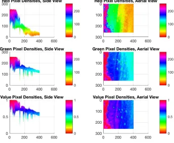
Figure 4.4: Frames used to test the relationship of lower pixel values for identified sharks in the Red, Green and Value arrays.

The first comparison was for ’Test Image 1’ which illustrated the 3D surface model for

the Red, Green and Value arrays. It can be seen in this image that the frame is from a

camera with a wide angle lens. The shark can be seen clearly in the middle of the frame

and is the darkest object in the frame. The upper sides of the image contain some glare

and there is reflection on the water due to the angle the camera is making with the water

and the sky above. The water is a much darker green than the original test image and

(56)

Figure 4.5: 3D surface model for Red, Green and Value arrays for test image 1 at side and aerial views.

As illustrated above the Red model does not display the peak where the shark is located

in the image. However the Green and Value display similar results and illustrate where

the peak for the shark is. There are also narrower peaks in the Green and Value plots

that represent the shadows in the waves.

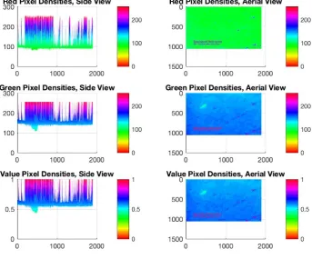
’Test Image 2’ contains nine sharks swimming in a light blue coloured ocean. There is

some whitewash to the left of the frame and the water has a darker shade of blue towards

(57)

[image:57.595.122.467.97.379.2]

Once again the Red model has failed to display the peaks where the sharks are, whereas

the Green and Value models depict the sharks location by the lighter shades of blue in

the colour map. The Value model appears to depict the sharks more clearly than the

Green model.

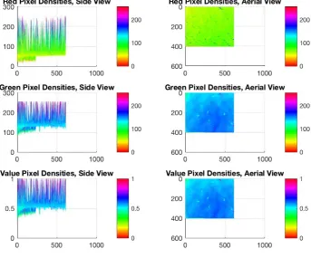
’Test Image 3’ contains one shark in the top left corner. The water is a greeney-blue

colour and there is some reflection from the sun on the tops of the waves. There is also

(58)

[image:58.595.122.466.97.382.2]

The Red model once again proves to be not of any use. The Green and Value models

both clearly depict the shark.

’Test Image 4’ contains seven sharks scattered throughout the frame. The water is a dark

(59)

[image:59.595.122.466.97.382.2]

4.3 Colour Space Thresholding 41

The Red model is clearly inadequate for using as a thresholding condition to detect the

shark blobs. The Green and Value channels appear to be the most reliable channels

suitable for pixel thresholding.

4.3

Colour Space Thresholding

From the tests performed in the previous section it can be assumed that Value pixel

density thresholding can be implemented to segment the shark blobs. Although this

might allow for some unwanted blobs, further blob analysis techniques can be utilised

to reject the false detections. To test the colour space thresholding for the test images,

threshold values were chosen after analysing the 3D surface models. The thresholds di↵er

for each image because of the di↵erent environments and colouring of the water. The

threshold values used were:

(60)

2. Test Image 2 = 0.551

3. Test Image 3 = 0.543

4. Test Image 4 = 0.504

The following pseudo code shows how anything over the cut-o↵pixel value in the Value

array is set to 0. It then converts the image to a binary map, performs some basic

morphology operations and then overlays the outline of the detected blobs over the original

image:

Algorithm 2 Display Blob Outlines on Original Image

procedure Imread(f rame)

2: framehsv rgb2hsv frame

Value (:,:,3)framehsv

4: fori = 1:size(Value,1)do

for j = 1:size(Value,2)do

6: if Value(i,j)>threshold then Value(i,j) = 0

BW imbinarize(Value)

8: BW imdilate(BW)

BW imfill(BW)

10: BW bwperim(BW)

BW imdilate(BW)

12: frame(BW) 255

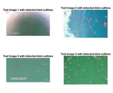
Display Test Images with detected blob outlines

(61)

[image:61.595.121.486.79.380.2]

Figure 4.9: Detected blob outlines overlaid on original image using Value pixel thresholding.

By determining an appropriate threshold for the Value pixel value, the majority of the

image can be ignored and only dark coloured blobs are left. The Value pixel is a number

between zero and one, where the closer to the zero the value is the darker the pixel is.

So everything above the threshold is therefore set to zero, and when the resulting image

is ’binarized’, all pixels with a value greater than zero are set to one. This is very basic

blob analysis and can be e↵ectively used in a controlled environment where the object of

interest is a unique colour to that environment.

However, there are plenty of blobs that have been detected that fell below the desired

threshold that are not sharks. This can be because of shadows in the waves or rocks in

the water. To help filter out all the unwanted blobs, further morphological operations can

be put in place to discard the false positives. Functions such as determining the minimum

blob area size and maximum area size are particularly useful for clearing up noisy data.

The above demonstrations illustrate that by applying a threshold to the Value array from

the HSV colour model of the frame, sharks can be detected and their blobs parsed to the

(62)

4.4 Adaptive Thresholding 44

project will concentrate on first detecting all the blobs under a given threshold for each

frame.

4.4

Adaptive Thresholding

The problem with applying a constant threshold to the data is that with each frame of

the video the environment can change. An adaptive threshold method was determined

and applied to automatically calculate the appropriate threshold for each frame. This was

achieved by representing the data from the Value array as a histogram and calculating

when the derivative was greater than a certain value starting from 0 and determining the

forward di↵erence. Because this method was tested with di↵erent pictures and videos

with di↵erent resolutions, an adaptive derivative formula was determined to calculate the

derivative threshold for each frame:

DerivativeT hreshold= f ramewidth⇤f rameheight

1500 (4.1)

The pseudo code for this loop can be represented as follows:

Algorithm 3 Calculate Threshold for Regions of Interest

procedure H = imhist(V alue)

D zeroslength(H,1)

3: fori = 1:length(H) do

D(i) H(i)-H(i+1)

if i == 255 then

6: break

if D(i)<(size(Value,1)*size(Value,2))/-1500 then

Threshold i/256

This method was used because it isolates the darker objects in the image. From the

data obtained, it was noticed that sharks were consistently a darker colour than the

surrounding water. This threshold calculation works well when the frame is made up of

bright scenes such as water, whitewash and sand. Due to the lack of data this method was

unable to be tested when there were cli↵s or rocks in the scene. The calculated threshold

(63)