A sub-catchment based approach for modelling nutrient dynamics and transport at a river basin scale

A Sub-Catchment Based Approach for Modelling Nutrient

Dynamics and Transport at a River Basin Scale

Md Jahangir Alam1&Dushmanta Dutta2

Received: 13 August 2015 / Accepted: 8 September 2016

#Springer Science+Business Media Dordrecht 2016

Abstract The prediction of nutrient pollution at realistic details is difficult due to lack of proper description of inherent processes in modelling tools. To overcome that this study has adopted a process based approach to build a semi-distributed model to simulate nutrient pollution in changing environment. The model was built to describe: (1) nutrient generation process in the catchment with consideration of different aspects of external and internal sources, (2) nutrient release from surface to the waterways via runoff and soil erosion, and (3) in-stream transport and chemical reaction process. The key novelty of this research is the linking of the nutrient generation process with transport mechanism for modelling nutrient dynamics at a basin scale. A flow capacity based approach was introduced to determine nutrient export from catchment to the waterways, which was useful to achieve the high resolution outputs from the model. The model performed reasonably well to represent the behaviour of nutrient in high flow events as well as in seasonal flow in two catchments located in distinct hydro-climatic regions. The study has shown that the nutrient model is suitable for predicting actual nutrient pollution in rivers for both high flow and seasonal flow under different hydro-climatic conditions. By simulating organic and inorganic nutrients separately, the model allows to estimate river water quality status in detail.

Keywords Nutrient pollution . Process-based modelling . Soil erosion . Catchment and in-stream process . River basin

1 Introduction

The quantification of nutrient pollution is one of the major issues in water resources manage-ment (Panagopoulos et al. 2011; Dutta et al.1998). Over the past few decades, nutrient DOI 10.1007/s11269-016-1500-x

* Dushmanta Dutta [email protected]

1 _{University of Southern Queensland, Darling Heights, QLD, Australia}

2

pollution has impacted river water quality mainly for land use change, agricultural practices and increases of pollution sources (Whitehead et al.1998a; Guse et al.2015). Accounting the inherent processes is necessary for modeling the catchment behavior and predicting the pollution level at higher spatio-temporal resolutions, which is the main focus in this research. Mostly the current modelling tools are conceptual in nature, developed for planning best management practice. This type of models are suitable for estimating the nutrient loads on an annual basis. They do not account hydrologic response and transport processes hence are unable to predict the nutrient level in higher spatio-temporal resolutions. Some of the tools have been improved or extended to predict nutrient level at a monthly or, daily time scale, such as, modelling tool E2 (Perraud et al. 2005) and Water and Contaminant Analysis and Simulation Tools (WaterCAST) (Cook et al.2009). Similar conceptual models were developed for European catchments such as Modelling Nutrient Emissions in River Systems (MONERIS) (Venohr et al.2011). Such models are comparatively simple to build (Tzoraki et al. 2014). However, using simple methods such as Event Mean Concentration (EMC) method or rate based approach the prediction of nutrient releases cannot be achieved at realistic details in changing environment. To overcome the situation this study has adopted a process-based nutrient modeling approach, which was emphasized in many studies. For example, a national level Australian study highlighted that due to the unavailability of proper models the effects of upstream flow processes and in-stream mechanisms on blue green algal growth remained unknown for many inland rivers in Australia (Croke and Young2001).

of in-stream transport processes in a newly developed model. A sub-catchment based approach is trialled to test the suitability of the different components. The research was aimed at developing and implementing a process-based nutrient model at an hourly time-step by incorporating the above-mentioned three attributes and demonstrating its suitability in catch-ment scale nutrient simulation through real-world applications.

This paper describes the sub-catchment based nutrient model and its applications in two distinct hydro-climatic regions in Japan and Australia for producing various nutrient fluxes at a basin scale.

2 Modelling Approach

The nutrient model was built within an existing process-based and distributed hydrological model called IISDHM, (Jha et al.2000; Dutta et al.2000,2006; Asokan and Dutta2008; Dutta and Nakayama2009; Kabir et al.2011). There are advancements made in alternative hydro-logical modelling approach using artificial neural network and optimizing techniques such as genetic algorithm (Taormina and Chau2015; Saeidifarzad2014; Wu et al.2009; Chen et al.

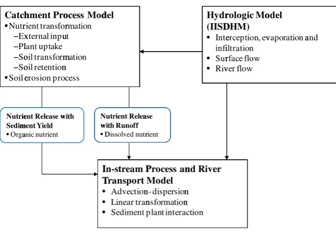
2015; Chau and Wu2010). However, such models are based on analysis of historical data, which are out of the scope. Hence IISDHM is chosen as it is a robust model for deterministic modelling similar to other distributed hydrological models such as MIKESHE. IISDHM mathematically represents the key components of the hydrologic cycle using physical governing equations and then simulates the movement of water using the principles of conservation of mass and momentum. The hydrologic components are grouped into five distinct modules: (i) Interception and evapotranspiration simulation, (ii) Unsaturated zone flow simulation, (iii) Saturated zone flow simulation, (iv) Overland flow simulation and (v) Channel network flow simulation. The IISDHM was used to simulate catchment runoff and estimate river discharges. The model solves Saint-Venant’s equations for continuity and momentum to compute surface and river flow. The kinematic wave method was used to approximate flow using an explicit finite difference solution scheme. The explicit model is conditionally stable by satisfying the Courant number (Chow et al. 1988). The IISDHM provides input of hydrologic flow for sub-catchment based modelling. Figure1 shows the conceptual framework of the integrated model.

3 Catchment Nutrient Model

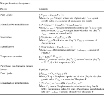
The catchment nutrient model estimates inorganic soluble nutrient release from different land uses (Alam and Dutta2013). The net nutrient generation is estimated based on generation rate by accounting transformation process in the soil layer under different soil moisture conditions. The nutrient module includes both nitrogen (N) and phosphorous (P) models. TheNmodel estimates the rate of net mineralization ofN, denitrification and nitrate (using the equations for different processes as shown in Table 1). The P model estimates the rate of net mineralization of Ptaking into account various processes in the soil including the adsorption and desorption of inorganic Pand weathering and precipitation of mineral P, and the output is inorganic soluble reactive P (PO4-P). The equations for different

processes included in thePmodel are shown in Table1.

SMD=SMDMax) and 1 when the soil is in saturation.SMIandSMDhave been calculated from

the following equations (Whitehead et al.1998a; Finkele et al.2006):

dSMD

dt ¼−PeffþET ð8Þ

SM I¼SM Dmax−SM D SM Dmax

ð9Þ

Where

Peff(rain-interception-runoff) Effective rainfall

ET Evapotranspiration.

Using Table1, the final equations for soluble nutrients at any timetcan be expressed as:

d

dtðN H4−NÞt¼ d

dtðExtNN H4þN etNMina−NN H4UptakeÞ ð10Þ

d

dtðN O3−NÞt¼ d

dt ExtNN O3þNitrification−N O3Uptake−Denitrification

ð11Þ

d

dtðPO4−PÞt¼ d

dtðExtPþN etPMina−PUptakeÞ ð12Þ

Where, NH4-N, NO3-N and PO4-P are ammonium, nitrate and dissolved phosphate,

respectively; ExtNH4,ExtNO3 andExtP are external inputs ofNNH4,NNO3and Prespectively,

which may include fertilizer application, atmospheric deposition or sewage disposal or other forms of input depending on catchment characteristics.

Catch

•Nutr

−Ex

−Pl

−So

−So

•Soil e

Nutrie Sedim

•Orga

hment Pro

rient transfor xternal inpu lant uptake oil transform oil retention erosion pro

ent Release w ment Yield

anic nutrient

ocess Mod

rmation ut

mation n

cess

I T

• • •

with N w

•D del

In-stream P Transport

Advection Linear tran Sediment

utrient Relea with Runoff

Dissolved nutr

Process an Model

n- dispersion nsformation plant intera

ase

rient

Hydr (IISD

• Inte

infi

• Sur

• Riv

nd River

n n

ction

rologic Mo DHM)

erception, ev iltration rface flow ver flow

odel

vaporation aand

The nutrients build up on the catchment surface through generation processes and are released with runoff. The release depends on the function of runoff. With this hypothesis, an export coefficient based nutrient release was introduced, which is a function of flow as shown in Eqs. (13–15).

d

dtðN H4−NÞrelease¼ d

dtðN H3−NÞt*Uw ð13Þ

d

dtðN O3−NÞrelease¼ d

dtðN O3−NÞt*Uw ð14Þ

d

dtðPO4−PÞrelease¼ d

dtðPO4−PÞt*Uw ð15Þ

The export coefficientUWhas been defined as below.

UW¼aQb ð16Þ

Where

a coefficient for soil and land cover effects

Table 1 Equations of nitrogen and phosphorus transformation process in soil layer (Whitehead et al.1998a)

Nitrogen transformation process

Process Equations

Plant Uptake d

dtNuptake¼CN upuiXN(1)

Where,CN up= Nitrogen uptake rate of plant (day− 1

),ui= plant

growth index,XN= amount of ammonium and nitrate

Mineralization-immobilization d

dtðN etNMinaÞ ¼CNminaSM I−CNimmXNamm(2)

Where,CN mina= Nitrogen mineralization rate (g day− 1

),SMI= soil moisture index,CN imm= Nitrogen immobilization rate (day−1),

Xamm= amount of mineralizedN

Nitrification d

dtNitrification¼CnitriXN H4−N(3)

Where,Cnitri= Nitrification rate (day−1),XN H4−N= amount of

AmmoniumN

Denitrification d

dtDenitrifcation¼CdeniXN O3−N(4)

Where,Cdeni= Denitrification rate (day−1),XN O3−N= amount of

NitrateN

Temperature correction Cn¼1:047ðθs−20ÞCr(5)

Where,Cn= rate of reaction (day−1),Cr= rate of reaction (day−1)

at 20 °C,θs= Soil temperature (°C)

Phosphorus transformation process

Process Equations

Plant Uptake d

dtPUptake¼CPupuiXPO4−P(6)

Where, CP up = Phosphorus uptake rate of plant (day-1), ui = plant growth index,XPO4−P= amount of Phosphate P

Mineralization-immobilization d

dtðN etPMinaÞ ¼CPminaSM I−CpimmXPO4−P(7)

b power factor

Q flow in m3/s.

3.1 Soil Erosion and Sediment Yield Models

The nutrient model includes the soil erosion and sediment yield model to compute soil bound nutrient (Organic N and P) release associated with soil erosion process. After estimating sediment load from each sub-catchment, soil bound nutrient release is calculated by multiply-ing the nutrient content with sediment load.

The estimation of soil erosion and sediment yield was carried out using Universal Soil Loss Equation (USLE) (Weischmer and Smith 1978) based models RUSLE (Renard et al. 1991,

1996) and MUSLE (Williams 1975; Williams and Berndt 1977). The RUSLE can be expressed by Eq. (17).

As¼RKLSCmPs ð17Þ

Where

As Average annual soil loss predicted (ton ha−1) R Rainfall runoff erosivity factor (MJ mm ha−1h−1)

K Soil erodibility factor (ton ha hr MJ−1ha−1mm−1)

L Slope length factor

S Slope steepness factor

Cm Cover management factor Ps Support practice factor.

The method is suitable for sub-catchment scale analysis (Weischmer and Smith1978) and Bhattarai and Dutta (2008) demonstrated its suitability for estimating soil erosion at a monthly time scale. The fraction of the total amount of soil erosion, at the catchment outlet, is determined by multiplying the soil erosion with the term called soil delivery ratio. The soil delivery ratio is determined using the following equation (Bhattarai and Dutta2007).

DR¼exp −γ Xm

i¼1

li aLiS0i:5

!

ð18Þ

Where

DR Soil delivery ratio i catchment cell

γ a constant for given catchment

aL a constant for land use type S surface slope

l the travel distance.

The Modified Universal Soil Loss Equation MUSLE (Williams1975; Williams and Berndt

1977) was used for the upper catchment of the Latrobe River, which is as below.

Sy¼a1ðQVÞb1KLSCmPs ð19Þ

Sy sediment yield Q discharge (m3s−1)

V Volume in (m3)

a1andb2constants 11.8 and 0.56 respectively K Soil erodibility factor

L Slope length factor

S Slope steepness factor

Cm Cover management factor Ps Support practice factor.

3.2 Estimation of Soil Bound Nutrients

The soil bound nutrients were estimated using the following equations (Leon et al.2001).

NSED¼NSCNYSEDER ð20Þ

PSED¼PSCNYSEDER ð21Þ

ER¼mYySEDTf ð22Þ

Where

NSED nitrogen transported by sediment (g s−1) NSCN nitrogen content in soil (g per g soil). Similarly PSED phosphorus transported by sediment (g s−1) PSCN phosphorus content in soil (g per g soil) YSED sediment yield (g s−1)

ER nutrient enrichment function

mand

y

are enrichment coefficients

Tf correction factor for soil texture (e.g. 0.85 for sand, 1.0 silt, 1.15 for clay and 1.5 for

peat).

3.3 River Nutrient Dynamics and Transport Model

Where

V element volume

c nutrient concentration

Ac element cross-section area E longitudinal dispersion coefficient

x along longitudinal space unit

t time

U average velocity

r reaction rate

p internal sources/sinks

s external or lateral sources/sinks.

The nutrient loads from each sub-catchment are used as input boundary conditions. The external input includes both inorganic and organic or soil bound nutrient from catchments.

3.3.1 Solution of Nutrient Transport Equation for River Network System

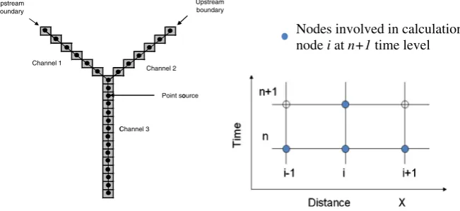
An explicit finite difference solution scheme was used to solve the mass balance Eq. (23) by discretizing the computational domain in space and time (Fig. 2) for calculation of nutrient concentration at each river grid. The explicit scheme is not as robust as an implicit scheme. However, the scheme is simple and easy to construct and computation-ally efficient. The results are affected by the scheme if the stability criteria are stratified. This was ensured in the model. The numerical form of the differential equation (Eq.23) is shown in Eq. (24).

cnþ1

i −cni

Δt ¼

AcE

ð Þi;iþ1 cniþ1−cni

ViΔx þ

AcE

ð Þi−1;i cni−1−cni

ViΔx þ

Qi−1cni−1−Qicni

Vi þ

ricni þpi

þ si

Vi ð

24Þ

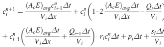
By taking average of the cross-sectional area and dispersion coefficientEbetween interface grids(i,i + 1)and(i,i-1)the Eq. (24) takes the form of Eq. (25), which achieves steady state condition in each time step to ensure model stability.

Channel Upstream boundary

C 1

Channel 3 Channel 2

Point so Upstream boundary

ource

Nodes involved in calculation for node i at n+1 time level

cnþ1

i ¼

AcE

ð Þavgcniþ1Δt

ViΔx þ

cn i 1−2

AcE

ð ÞavgΔt

ViΔx −

QiΔt

Vi

þcn i−1

AcE

ð ÞavgΔt

ViΔx þ

Q_i−1Δt Vi

−ricniΔtþpiΔtþ

siΔt

Vi

ð25Þ

Where, negative sign denotes reaction component (rici) for decay.

The equation can be further re-arranged as:

cn_iþ1¼cn_iþ1λþcn_ið1−2λ−γÞ þcn_i−1ðλþγÞ−ricniΔtþpiΔtþ siΔt

Vi ð

26Þ

Where

λ _{Diffusion number =}ðAcEÞavgΔt

ViΔx

γ Advection number or Courant stability condition =QiΔt

Vi

In the model, longitudinal dispersion coefficient, E is calculated using the following equations developed by Fischer et al. (1979).

E¼0:011U

2_W2

H U* ð27Þ

U*¼ ffiffiffiffiffiffiffiffiffiffiffiffigH S0

p

ð28Þ

Where

U Flow velocity m/s

W Channel width (m)

H Mean depth of water (m)

U* Shear velocity (m s−1)

g Acceleration due to gravity (m s−2)

S0 Channel bed slope.

3.3.2 In-Stream Chemical Reactions

The term (rc + p)represents the reaction component in the mass balance Eq. (23), where

rc is the total reactant, linearly dependant on the constituent’s concentration and p

represents the internal constituents - source and sink (Chapra 1997). Table 2 shows how these reaction terms (rc andp) have been represented for each constituent.

4 Study Areas

4.1 The Saru River Basin

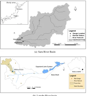
The Saru River is situated in Hokkaido, which is in the northernmost area of Japan (Fig.4a). It originates at Mount Memuro (Nakamura and Kikuchi1996) and passes through an alluvium plain in the downstream region, and has a catchment area of 1,350 km2. With a trunk river channel length of 104 km and a bed slope ranging from 1/500 to 1/800, it is one of the steepest river systems in this region of Japan (Yoshikawa et al.2006). The basin is known as rocky, with a thin top soil layer (about 1 m) (Yoshikawa et al.2006). The land use is predominantly forest (92 %). Other land use types are agriculture including rice, fruits and vegetable growing fields, and some urban features.

Flooding is a recurring phenomenon in the Saru River. Huge amounts of sediment and nutrients were carried out by the river during heavy floods in 2001. Water quality measure-ments of these two flood events in the basin were used for the model calibration and validation.

4.2 The Latrobe River Basin

In contrast, the Latrobe River is situated in a very dry temperate region of the Victorian State in Australia. It drains a catchment area of 4,500 km2 (Fig. 4b). The river has significant socio-economic and environmental values for the region, which is used for supplying water to some major thermal electric power generation plants and other

Table 2 Equations for in-stream reaction process (after Chapra1997)

Constituent Equations

OrganicN(NORG) dN_dtORG¼α1ρA−β3NORG−σ4NORG(27)

The termα1ρAis accumulation due to algal respiration, whereα1ρis

accumulation rate ofNORGdue to algal respiration (day−1) andAis mass

of algae (mg l−1),β3is decay coefficient ofORG-Nandσ4is settling

rate ofNORG.

The simulation of algal biomass can be carried out using following equation.

dA

dt¼μA−ρA−σ 1 HA(30)

Where,μis growth rate of algal biomass (day−1_{),ρis loss rate of algal biomass}

due to respiration,σ1settling rate of algae (m− 1

) andHis water depth (m). AmmoniumN(NNH4) dN_dtN H4¼β₃NORG−β₁NN H4þσH3NN H4−Fα1μNN H4(31)

Where,β3is decay rate ofORG-N,β1is rate of nitrification ofNNH4,σ3 is

accumulation rate ofNNH4due to resuspension of sediment,Fα1μNNH4is

total loss ofNNH4for algal growth,α1μis loss rate ofNNH4for algal growth

andFis fraction.

NitriteN(NNO2) dN_dtNO2¼β₁NN H4−β₂NNO2(32)

where,β2is rate of nitrification ofNNO2

NitrateN(NNO3) dN_dtNO3¼β₂NNO2−ð1−FÞα1μNNO3(33)

OrganicP(PORG) dP_dtORG¼α2ρA−β4PORG−σ5PORG(34)

where,α2ρis rate of accumulation ofPORGdue to algal respiration,β4is a decay

rate ofPORG,.σ5is settling rate ofPORG

DissolvedP(PDISS) dPDISS

dt ¼β4PORGþσH2PDISS−DISSα2μPDISS(35)

where,β4decay rate ofPORG,σ2is accumulation rate ofPDISSdue to re-suspension

regional industries (LVWSB 1986). The land use types are mainly forest (41 %), dairy farm (44 %), natural grazing pasture, mining and cropping land. Built up areas are relatively small.

The upper and relatively hilly catchment is selected for modelling. The river originates on a hilltop and incises through the undulating landscape before steps down to relatively flat area from topographic elevation 274 to 59 m. The land use types are mainly production forest and grazing pasture in this upper catchment.

5 Modelling in the Saru River Basin

5.1 Model Setup

The original 250-m grid of Digital Elevation Model (DEM) for the study area was hydrolog-ically corrected using the hydrological assessment tool within ARCGIS. The river network was derived from the corrected DEM using GIS to form the river model. Each branch of the river network was indexed and every node was defined with cross-section geometry. The catchment was divided into 17 sub-catchments coinciding the inflow nodes from 17 branches to main trunk of the river network.

Table 3 Model state variables

1) Plant uptake of nitrogen 8) Plant uptake ofP

2) OrganicN(NORG) 9) OrganicP(PORG)

3) Net mineralization ofP 10) Net mineralization ofP

4) Net nitrification ofN 11) PhosphateP(PO4-PorPDISS)

5) Net denitrification ofN 12) Suspended sediment 6) AmmoniumN(NNH4)

7) Nitrite + NitrateN

The time series inputs were hourly rainfall and daily evaporation data for hydrological simulation. The RUSLE method was used to estimate soil erosion. Based on the sediment delivery ratio the sediment yield was predicted. TheKfactor was assumed for sandy layer of the top soil of the catchment.LSparameter depends on the slope length and steepness of the sub-catchments. Cmand Psfactors are the average value for the different land use

types. The suspended sediment measured at Horokeshi station for three consecutive days during the flood event was used for comparison with the model results.

The calculation of nutrient release from sub-catchments involves estimation of organic and inorganic nutrients. The soil bound organic nutrient was estimated as sediment yield multiplied with nutrient concentration in eroded soil. The inorganic nutrient release was estimated based on different input rates of nutrient generation and transformation. The input rate of N andP mineralization from different land uses and their corresponding

(b) Latrobe River basin (a) Saru River Basin

transformation rates were obtained from literature such as Whitehead et al. (1998b). However, the information is very scarce for the Pprocess. The observedPuptake rate for different crops and grassland for the catchments of UK and USA as reported in Wade et al. (2007) has been used as a guide for determiningPuptake rate. The details of the input parameters are also provided in Table4.

The SMI was assumed to be at constant level 1, considering the wet/saturated condition of the catchment during the flood events. The effect ofSMIover short period would not change. The reaction coefficients in the river module were judged based on available information in the text book of Chapra (1997).

5.2 Model Accuracy and Sensitivity Analysis

An assessment of numerical accuracy and sensitivity analysis of model parameters were undertaken prior to the model calibration and validation. A parameter perturbation method was used for the sensitivity analysis. The numerical accuracy was assessed by analyzing mass balance and verifying the stability criteria. The numerical stability criteria of the Courant condition and the Diffusion number were estimated during simulation, which should be less than 1 and 0.5, respectively at each time step. For mass balance, a test simulation was carried out using synthetic time series boundary conditions applied at each upstream point of the Saru River network. The constituent model was run without chemical reaction. The simulated results had 8 % and 6 % numerical errors forN andP,respectively, and less than 4 % for discharge. These errors margins of less than 10 % are considered to be acceptable. The difference in error forN

andPwas mainly due to the difference in magnitude for input loadings.

The sensitivity tests suggest that the chemical reaction coefficients have a significant impact on the nutrient level at river network system and these are to be judged during calibration process. The export coefficients of surface model have high impacts on nutrient loading, which are also to be judged during calibration. It is noteworthy to mention that the adequacy of organic nutrient loading calculation depends on the calibration of the sediment modelling and assumption of nutrient content in eroded soil.

Table 4 Input for catchment nutrient process modelling

Input Latrobe River Saru River

Grazing pasture Production Forest

Paddy Field Grassland Forest

NFertilizer (kg ha−1year−1) 60 – 150 – –

NUptake (kg ha−1year−1) 35 5 95 35 40

NMineralization (kg ha−1_year−1_{) 60 40 50 40 40}

Nitrification (kg ha−1_year−1_{) 20 10 30 15 15}

Denitrification (kg ha−1_year−1_{) 1 1 19 1 1–4}

PUptake (kg ha−1_year−1_{) 12 – 25 12 –}

PMineralization (kg ha−1_year−1_{) 12 10 0 0 0}

5.3 Model Calibration and Validation

The model was calibrated against observed streamflow and sediment and nutrient fluxes. The calibration was first undertaken against streamflow using Manning’s roughness coefficient for both overland and river flow. An extreme flood event in September 2001 was used for the calibration. A relatively lower magnitude flood event occurred during August 2001 was selected for model validation. These two flood events were selected due to the availability of high quality observed data of suspended sediment and nutrient fluxes, collected by intensive field sampling during the flood events. The calibrated parameters were used in the validation without any further adjustment. The model results were compared against the observed records for evaluating performance using a number of statistical evaluation criteria (Van Liew et al.

2005and Stehr et al.2008) (Table5).

5.4 Results

(a) Hydrological simulation results

The hydrological simulation was carried out for generating catchment runoff and river discharges. The comparisons of the observed and simulated discharges at Horokeshi station during the calibration and validation are shown in Fig.5a and b, respectively. The peak flow and the overall shape of the hydrographs match very well with the observed data during the period of calibration. The model performance was similar in the valida-tion period as well. TheNSEvalues were 0.87 and 0.94 for the calibration and validation periods, respectively (Table6).

(b) The soil erosion and sediment yield

The samples of suspended sediments during the field measure were taken in varied intervals ranging from 15 min to a few hours. The data was averaged to daily interval and compared with the RUSLE model output as shown in Fig.5c and d. The simulated time series of suspended sediments show close agreement with the observed data for both calibration and validation periods. Although number of observed data were limited, the agreement between the observed data and simulated results was highly satisfactory. (c) Nutrient simulation results

The observed data were available in the form of total nitrogen (TN),NH4andNO3and

total phosphorus (TP), PO4 and dissolved phosphate (DPO4). From these datasets,

organic N and P were derived as a difference between total and inorganic N andP, respectively. The interval of data varied from 15 min to few hours for consecutive 3 days during each of the two flood events in August and September 2001. The 15-min interval data was averaged to hourly interval and compared with the model results.

The model computes nutrient concentration at each node of the river network system. The results were compared with the observed nutrient records at Horokeshi gauge and

Table 5 Evaluating criteria for model results against statistical indices

Good Satisfactory Not satisfactory

NSE >0.75 0.75–0.36 <0.36

Correlation coefficient (R2_{) >0.75 0.75–0.36 <0.36}

presented with stream flow in the same plot for showing the relationship between the streamflow flow and nutrient fluxes.

Figure 6a–d compares the simulated and observed nutrient levels in the Saru River during calibration. The simulated results agreed well with the observed data. The profiles of ORG-NandORG-Pshow the rise and fall varying with the stream flow indicating strong co-relation between river flow and nutrient loads. The initial condition was set to zero level from where the concentration was rising with the increase of nutrient loading from the sub-catchments and started decreasing with the

(c) Suspended sediment during calibration

0 200 400 600 800 1000 1200 1400 1600 1800 2000 08-Sep FL o w ( m 3 /s ) 0 2000 4000 6000 8000 10000 12000 7/ Co n c . ( m g /l )

10-Sep 12-Se

/

ep 14-Sep 1 Date (2001) 13/09 16-Sep Avg rainfall Observed Simulated 0 500 1000 1500 2000 2500 3000 3500 4000 16/09

(d) Suspended sediment during validation

R a in fa ll ( m m ) 1 1 2 2 Fl o w (m 3 /s ) Fl ow ( m 3 /s) Co n c e n tr a ti o n ( m g /l ) 0 50 00 50 00 50 00 0 1000 2000 3000 4000 5000 20/08 21/ Date (2001)

/ 08 22/08 23/ Date(2001)

Simulated Observed

/ 08 24/08 25/

Sed. Sim. Sed. Obs. Q Sim. 0 200 400 600 800 08 Fl ow ( m 3 /s ) Date(2001) Sed. Sim. Sed. Obs. QSim. 09 10/09 60 50 40 30 20 10 0

21-Aug 22-Aug 23-Aug 24-Aug 25-Aug 26-Aug

(a) Discharge during calibration (b) Discharge during validation

18-Sep

3

Fig. 5 Comparison of simulated and observed discharge and suspended sediments during calibration and

validation at Horokeshi, the Saru River

Table 6 Statistical indices evaluating model performance for the Saru River

Simulation Period Parameter RRMSE MAE PBIAS NSE R2

Sep 2001 Flow 0.31 55.97 7.47 0.94 0.95

Sus.sed (SS) 0.50 1668.13 33.00 0.80 0.80

ORG-N 0.24 2.04 −18.07 0.70 0.73

NO3-N 0.05 0.02 1.00 0.67 0.60

ORG-P 0.23 0.34 −17.98 0.72 0.79

P04-P 0.17 0.23 −6.96 0.78 0.66

Aug 2001 Flow 0.15 17.74 1.34 0.87 0.90

Sus.sed 0.19 205.99 −3.51 0.98 0.99

ORG-N 0.12 0.08 0.51 0.42 0.87

NO3-N 0.03 0.01 1.81 0.47 0.60

ORG-P 0.19 0.04 6.99 0.52 0.57

(a)

(b)

(c)

(d)

(e)

(f)

(g)

(h)

0 500 1000 1500 2000 2500 3000 3500 4000 4500 5000 0 5 10 15 20 25 30

7/09 9/09 11/09 13/09 15/09 17/09

Fl ow ( m 3/s) Co n c . ( m g /l ) Date (2001) ORG-N Sim. ORG-N Obs. Q. Sim. 0 100 200 300 400 500 600 700 800 900 0.00 0.50 1.00 1.50 2.00 2.50 3.00 3.50

21/08 22/08 23/08 24/08 25/08 26/08

Fl o w m 3/s) Co n c . ( m g /l) Date (2001) ORG-N sim. ORG-N obs. Q Sim. 0 500 1000 1500 2000 2500 3000 3500 4000 4500 5000 0 0.1 0.2 0.3 0.4 0.5 0.6 0.7 0.8 0.9 1

7/09 9/09 11/09 13/09 15/09 17/09

Fl ow ( m 3 /s ) Co n c . ( m g /l) Date(2001) NO3-N Sim. NO3-N Obs. Q. Sim. 0 100 200 300 400 500 600 700 800 900 0 0.1 0.2 0.3 0.4 0.5 0.6 0.7 0.8 0.9 1

21/08 22/08 23/08 24/08 25/08 26/08

Fl ow ( m3 /s) Co n c . ( m g /l ) Date(2001) NO3-N sim. NO3-N Obs. Q Sim. 0 500 1000 1500 2000 2500 3000 3500 4000 4500 5000 0 1 1 2 2 3 3 4 4 5 5

7/09 9/09 11/09 13/09 15/09 17/09

Fl ow ( m 3 /s ) Co n c . ( m g /l ) Date (2001) ORG-P obs. ORG- P Sim. Q. Sim. 0 100 200 300 400 500 600 700 800 900 0.0 0.1 0.2 0.3 0.4 0.5 0.6 0.7 0.8 0.9 1.0

21/08 22/08 23/08 24/08 25/08 26/08

Fl o w ( m 3/s) Co n c . ( m g /l ) Date (2001) ORG-P Obs. ORG-P Sim. Q Sim. 0 500 1000 1500 2000 2500 3000 3500 4000 4500 5000 0.0 0.5 1.0 1.5 2.0 2.5 3.0 3.5 4.0

7/09 9/09 11/09 13/09 15/09 17/09

Fl o w ( m 3 /s) Co n c . ( m g /l) Date (2001) PO4-P Obs. PO4-P Sim. Q. Sim. 0 100 200 300 400 500 600 700 800 900 0 0.1 0.2 0.3 0.4 0.5 0.6 0.7 0.8 0.9 1

21/08 22/08 23/08 24/08 25/08 26/08

Fl o w ( m 3/s ) Co n c . ( m g /l ) Date(2001) PO4-P sim. PO4-P Obs. Q Sim.

Fig. 6 Comparison of simulated and observed nutrients at Horokeshi during the periods of model calibration and

decrease of flow. The high intensity flood carried out huge wash off pollutant as reflected in the figure. Due to decay of NO3-N the profile was flattened, which

agreed well with the observed pattern. The model performance level was in the range from theBsatisfactory^to theBgood^level as presented in Table6. TheNSE

and R2 values are above 0.69 and 0.60 with the maximum values 0.77 and 0.79, respectively during calibration.

The model set up for the validation was same as the calibration except the period of simulation. The initial conditions for nutrient concentration at each river grids were set to zero for most of the pollutants. The simulated nutrient fluxes are presented in Fig.6e–h

along with the observed data. The results show the rising limbs match well with the observed data forORG-NandORG-PandPO4-P. The response of chemical reaction is

seen on the concentration level ofNO3-NandPO4-P,which shows the gradual decrease of NO3-NandPO4-Plevels at recession limbs. The model performance is within the range of

satisfactory and good levels (Table6). The concentration level ofNO3-Nmatched well with

the observed data in the recession limb of the hydrograph withNSEandR2values of 0.47 and 0.6, which are satisfactory. ThePBIASvalue is within the good range for all nutrient constituents in the calibration and validation.

6 Modelling in the Latrobe River

6.1 Model Set Up

A 1-km DEM was used to set up the hydrological model for the Latrobe River. The model also consists of the land use and soil maps. The model was calibrated against Manning’s roughness parameter. A runoff coefficient was used in determining surface runoff and a constant base flow was assumed to match the low flow, which is 1.9 m3s−1. For the Latrobe River basin, the simulation was carried out for a longer period. The data preparation for this application was similar to the Saru River application. The MUSLE was used for continuous simulation of sediment yield. Average Kvalue was assumed for soil types of the catchment.CmandPs

factors were assumed for the different land use types mainly forests and pasture. The input parameters for nutrient flux simulation are tabulated in Table 4 above. For pasture based grazing system thePapplication rate is 44 kg ha−1year−1in the Latrobe river region (Drysdale

1998; Nash and Halliwell1999). TheNapplication rate is from previous reference. The yearly input rate of fertilizer was uniformly distributed over the simulation period. A further analysis

0 0.2 0.4 0.6 0.8 1 1.2

May-07 Jul-07 Sep-07 Oct-07 Dec-07 Feb-08

S

M

I

nde

x

0 0.2 0.4 0.6 0.8 1 1.2

Aug-09 Mar-10 Oct-10 Apr-11

S

M

I

nde

x

on actual timing of fertilizer application is needed. The soil moisture index (SMI) was calculated based on rainfall, runoff and antecedent soil moisture condition. Figure7shows the seasonal variation ofSMIindex for the Latrobe River.

6.2 Model Calibration and Validation

The hydrological model was first calibrated using Manning’s roughness parameter and then, the sediment and nutrient modules were calibrated. A runoff coefficient was used in deter-mining surface runoff and a constant base flow was assumed to match the low flow, which is 1.9 m3s−1. The validation period was from September 2009 to end of July 2011.

0

10

20

30

40

50

60

70 0

10 20 30 40 50 60

Jun-07 Jul-07 Aug-07 Oct-07 Nov-07

Rain

fa

ll (

m

m)

Fl

o

w

(

m

3

/s

)

0

20

40

60

80

100 0

15 30 45 60

Aug-09 Jan-10 May-10 Sep-10 Jan-11 Jun-11

Rain

fa

ll (

m

m

)

Fl

ow

(

m

3

/s

)

Observed Simulated Rainfall

(b)

(a)

Fig. 8 Comparison of discharge at

Willow Grove, the Latrobe River

Table 7 Statistical indices for hydrological, sediment and nutrient model results at Willow Grove, the Latrobe

River

Parameters Period RRMSE MAE PBIAS NSE R2

Discharge Calibration 0.48 1.05 −3.00 0.66 0.74

Validation 0.55 1.79 −2.40 0.51 0.55

Sus.Sed Calibration 0.25 1.94 8.77 −0.10 0.04

Validation 0.57 4.26 30.61 −0.23 0.53

ORG-N Calibration 0.30 0.07 19.84 −0.73 0.01

Validation 0.59 0.15 36.95 −0.39 0.29

TP Calibration 0.38 0.01 20.41 −0.29 0.45

Validation 0.49 0.01 30.38 −0.22 0.52

NO3-N Calibration 0.18 0.05 −1.88 0.76 0.77

6.3 Results

(a) Hydrological model results

Figure 8 shows a comparison of the simulated and observed discharge at Willow Grove. By statistical measures the model shows satisfactory performance (Table7). The

NSE values are 0.66 and 0.51 and R2 values 0.74 and 0.55 for the calibration and validation periods, respectively.

(b) Sediment modelling results

Figure 9a–b shows the comparison of the observed sediment and MUSLE model

(a)

(b)

(c)

(d)

(e)

(f)

(g)

(h)

0 20 40 60 80 100 120 5 7 9 11 13 15 17 19

May-07 Jul-07 Aug-07 Oct-07 Nov-07 Jan-08

Fl ow ( m 3 /s) ) Co n c. ( m g/ l)

Sed. Sim. Sed. Obs. Q Sim.

0 20 40 60 80 100 120 0 5 10 15 20 25 30

Aug-09 Dec-09 Apr-10 Aug-10 Dec-10 Apr-11 Aug-11

Fl o w (m 3/s) Co n c. ( m g /l )

Sed. Sim. Sed. Obs. Q Sim.

20 0 40 60 80 100 120 0.15 0.2 0.25 0.3 0.35 0.4 0.45 0.5

Jun-07 Jul-07 Aug-07 Oct-07 Nov-07

Fl ow ( m 3 /s) Con c. ( m g/ l)

ORG-N Sim. ORG-N Obs. Q Sim.

0 20 40 60 80 100 120 0 0.1 0.2 0.3 0.4 0.5 0.6 0.7 0.8 0.9 1

Aug-09 Dec-09 Apr-10 Aug-10 Dec-10 Apr-11 Aug-11

Fl ow ( m 3/s) Co n c. ( m g /l )

ORG-N Sim. ORG-N Obs. Q Sim.

0 20 40 60 80 100 120 0.02 0.025 0.03 0.035 0.04 0.045 0.05 0.055 0.06

Jun-07 Jul-07 Aug-07 Oct-07 Nov-07

Fl ow ( m 3 /s) Co n c. ( m g /l )

TP Sim. TP Obs. Q Sim.

0 20 40 60 80 100 120 0 0.01 0.02 0.03 0.04 0.05 0.06 0.07 0.08 0.09 0.1

Aug-09 Dec-09 Apr-10 Aug-10 Dec-10 Apr-11 Aug-11

Fl o w (m 3/s) Co n c . (m g /l)

TP Sim. TP Obs. Q Sim.

0 20 40 60 80 100 120 0.00 0.20 0.40 0.60 0.80 1.00

May-07 Jul-07 Sep-07 Nov-07

Fl o w (m 3/s) C o n c. (m g /l)

NO3-N Obs. NO3-N Sim. Q Sim.

0 20 40 60 80 100 120 0.00 0.50 1.00 1.50 2.00 2.50 3.00

Aug-09 Dec-09 Apr-10 Aug-10 Dec-10 Apr-11 Aug-11

Fl o w (m 3/s) Con c. (mg /l )

NO3-N Sim. NO3-N Obs. Q Sim.

Fig. 9 Comparison of observed and simulated suspended sediment, ORG-N, TP and NO3-N at Willow Grove,

results at Willow Grove with the statistics presented in Table7. The sediment concen-tration is highly correlated to the discharge. However, there was not enough dataset to compare the model results particularly for the period of calibration. The results in the validation period are within the upper and lower range of the observed data with few observed data points outside of the range.

(c) Nutrient modelling results

Figures9c–fshow the comparison of model results forORG-NandTP.The model results could only follow the overall trend in observed ORG-N and TP level. The observed data is scattered, hence, a good performance could not be achieved by statistical measures (Table7). The levels ofORG-NandTPare dependent on the level of sediment yield, both cases represent similar trend (Fig.9).

The seasonal pattern ofNO3-Nlevel was predicted reasonably accurately by the model

(Fig. 9g–h)). The NSEandR2values during the calibration period are 0.76 and 0.77, respectively and those were 0.4 and 0.6, respectively for the validation.

7 Discussion

The model performed reasonably well in two different catchments demonstrating its ability to predict the nutrient levels under different hydro-climatic conditions. With the adequate mathe-matical representations of soil erosion and transport, and nutrient generation and transport along the hydrological flow paths within a process-based hydrological modelling framework, the model was able to simulate the sediment and nutrient fluxes reasonably well in high flow events. The high intensity measurements in the Saru River were useful to evaluate the adequacy of sediment and nutrient modelling in high intensity storm events. The model was also able to simulate long term seasonal pattern of sediment and nutrient levels in the Latrobe River.

The separation of nutrient generation process and transport in the modelling process has been effective in determining the different forms of nutrients loads including the sediment bound nutrients. Table8shows the contribution of nutrient from different components. From this table, it is seen that the organic loads are usually higher than inorganic loads in the Saru River but in the upper catchment of the Latrobe river the inorganicNload is higher than soil bound organicN, which is due to the fact that huge amount of sediment and nutrient loads were washed off during the high intensity storm events in the Saru River, whereas in Latrobe River the wash-off loads were relatively low.

Process-based nutrient models are generally complex relying on a large number of datasets. However, we could gather reasonably high intensity field measured data particularly for the Saru River to validate the model in predicting nutrient release in

Table 8 Total nutrient loads from different components

Period Organic N Load

Inorganic N load (kg)

Organic P Load

Inorganic P load (kg)

Saru River Calibration 1466430 65697 229379 190813

Validation 39819 11144 12742 9828

Upper Latrobe Calibration 18725 23527 1997 –

higher resolution. With the improvements in monitoring techniques, sampling methods and analysis techniques in the recent years, the quality and resolution of data required for such modelling are becoming available.

The study suggests that the soil erosion models can be further improved. Using soil delivery ratio is a relatively simple way to predict sediment dynamics. The ratio is a function of length, slope and a constant, which is a conceptual approach in deriving yield without accounting actual catchment process. The RUSLE method was replaced by MUSLE for the Latrobe River to take into account of overland flow effects on soil erosion and provide continuous output of sediment yield. The MUSLE is found to be more effective than RUSLE. However, this could be improved further if the hill slope soil erosion is coupled with sediment transport modelling. There is a scope to improve this component of the model in the future research.

8 Conclusion

We have presented the development and applications of a sub-catchment based nutrient model. The model accounts the processes of internal chemical reaction with soil-moisture and climate condition in estimating nutrient generation and release from different land uses. A function based approach was introduced to estimate dissolved nutrient release with runoff. Widely used empirical methods for soil erosion and sediment yield was used to estimate soil bound nutrient. The performance of the model in calibration and validation was quite acceptable for the two case studies. The model was able to predict the nutrient fluxes association with two short term record breaking flood events in the Saru River and the long term nutrient level in the Latrobe River. The model could provide output at an hourly interval, which was validated against observed data, showing realistic details of the nutrient dynamics. The statistical indices show satisfactory and good level performance for the Saru River. In spite of limited data, the model could reproduce the seasonal trend of nutrient level for the Latrobe River reasonably well. However, due to poor performance of sediment model, the actual profile of soil bondTP

and ORG-N could not be predicted well for the Latrobe River. There is a scope to improve the model by replacing the empirical approach with process oriented sediment modelling approach.

The study has shown that the nutrient model is suitable for predicting actual nutrient pollution in rivers. By simulating organic and inorganic nutrients separately the actual river water quality status could be known effectively. The application of the model can be extended to incorporate other pollutants such as bacteria.

Acknowledgements Authors greatly acknowledge the Civil Engineering Research Institute of Hokkaido and

Kitami Institute of Technology, Japan and Victorian Water Resources Database for data and several internal and external reviewers for their contribution to improve the manuscript.

Compliance with Ethical Standards

Funding The study was undertaken as part of a PhD research project at Monash University, Australia and

partially funded by the Asia Pacific Network for Global Change Research.

References

Abbott MB, Bathurst JC, Cunge JA, O’Connell PE, Rasmussen J (1986) An introduction to the European hydrological system - systeme hydrologique Europeen,‘SHE’, 2: structure of a physically-based, distributed modelling system. J Hydrol 86:61–77

Abrahamsen P, Hansen S (2000) Daisy: an open soil-crop-atmosphere system model. Environ Model Softw 15:313–330

Alam MJ, Dutta D (2013) Predicting climate change impact on nutrient pollution in waterways: a case study in the upper catchment of the Latrobe River, Australia. Ecohydrology 6(1):73–82 Arnold JG, Srinivasan R, Muttiah RS, Williams JR (1998) Large area hydrologic modeling and

assessment: part I. Model development. J Am Water Resour Assoc 34(1):73–89

Asokan S, Dutta D (2008) Analysis of water resources in the Mahanadi River Basin, India under projected climate conditions. Hydrol Process 22:3589–3603

Bhattarai R, Dutta D (2007) Estimation of soil erosion and sediment yield using GIS at catchment scale. Water Resources Management Journal 21:1635–1647

Bhattarai R, Dutta D (2008) A comparative analysis of sediment yield simulation by empirical and process-oriented models in Thailand. Hydrol Sci J 53(6):1253–1269

Chapra SC (1997) Surface-water quality modelling. WCB McGraw Hill, USA

Chau KW, Wu CL (2010) A hybrid model coupled with singular spectrum analysis for daily rainfall prediction. J Hydroinf 12(4):458–473

Chen XY, Chau KW, Wang WC (2015) A novel hybrid neural network based on continuity equation and fuzzy pattern-recognition for downstream daily river discharge forecasting. J Hydroinf 17(5):733–744

Chow VT, Maidment DR, Mays LW (1988) Applied hydrology, McGrawhill, USA

Cook FJ, Jordan PW, Waters DK, Rahman JM (2009) WaterCAST–Whole of catchment hydrology model an overview. MODSIM Congress, Cairns

Croke J (2002) Managing phosphorus in catchment, River Landscapes, Fact Sheet 11, Land & Water, Australia Croke J, Young B (2001) River contaminants: what are river contaminants and how can we effectively manage them for riverine and ecosystem protection?BRipRap^, River and Riparian Lands Management Newsletter, Land & Water Australia, Canberra, 20:1–6

DHI (2002) MIKE11: A modelling system for rivers and channels, Reference manual, DHI Water & Environment, Hørsholm, Denmark

Dise N (2004) An introduction to INCA: integrating nitrogen in catchment. Hydrol Earth Syst Sci 8(4):597–600 Drysdale G (1998) Dairy farm performance analysis 1996–97. Annual Report, DNRE, Melbourne

Dutta D, Nakayama K (2009) Effects of spatial grid resolution on river flow and surface inundation simulation by physically based distributed modelling approach. Hydrol Process 23:534–545

Dutta D, Das Gupta A, Ramnarong V (1998) Design and optimisation of a groundwater monitoring system. Ground Water Monit Remediat 18(1):139–147

Dutta D, Herath S, Musiake K (2000) Flood inundation simulation in a river basin using a physically based distributed hydrologic model. Hydrol Process 14:497–519

Dutta D, Herath S, Musiake K (2006) An application of a flood risk analysis system for impact analysis of a flood control plan in a river basin. Hydrol Process 20(6):1365–1384

Finkele K, Mills GA, Beard G, Jones DA (2006) National gridded drought factors and comparison of two soil moisture deficit formulations used in prediction of forest fire danger index in Australia. Aust Meteorol Mag 55:183–197

Fischer HB, List EJ, Koh RCY, Imberger J, Brooks NH (1979) Mixing in inland and coastal water. Academic, New York

Guse B, Pfannerstill M, Fohrer N (2015) Dynamic modelling of land use change impacts on nitrate loads in rivers. Environ Process 2(4):575–592

Hansen S, Jensen HE, Nielson NE, Svendson H (1990) DAISY. A soil plant system model. Danish simulation model for transformation and transport of energy and matter in the soil plant atmosphere system. NPO-Research Report A 10, Copenhagen

Jha R, Herath S, Musiake K (2000) River network solution for a distributed hydrological model and applications. Hydrol Process 14:575–592

Jones CA, Dyke PT, Williams JR, Kiniry JR, Benson VW, Griggs RH (1991) EPIC: an operational model for the evaluation of agricultural sustainability. Agric Syst 37:341–350

Kouwen N (1999) WATFLOOD/SPL8 Flood Forecasting System. Documentation and User Manual. Civil Engineering, University of Waterloo, Waterloo, Canada

Leon LF, Soulis ED, Kouwen N, Farquhar GJ (2001) Nonpoint source pollution: a distributed water quality modelling approach. Water Res 35(4):997–1007

Lunn RJ, Adams R, Mackay R, Dunn SM (1996) Development and application of a nitrogen modelling system for large catchments. J Hydrol 174:285–304

LVWSB (1986) The Latrobe River Basin, Water Resources and Aquatic Environment, a review, The Latrobe Valley Water and Sewerage Board, Australia

Nakamura F, Kikuchi S (1996) Some methodological development in the analysis of sediment transport process using age distribution of floodplain deposits. Geomorphology 16:139–145

Nash DM, Halliwell DJ (1999) Fertilisers and phosphorus loss from productive grazing systems. Aust J Soil Res 37:403–429

Panagopoulos Y, Makropoulos C, Mimikou M (2011) Diffuse surface water pollution: driving factors for different Geoclimatic regions. Water Resour Manag 25:3635–3660

Perraud JM, Seaton SP, Rahman JM, Davis GP, Argent RM, Podger GM (2005) The architecture of the E2 catchment modelling framework, MODSIM2005, 690–696

Radwan M, Willems P, El-Sadek A, Berlamont J (2003) Modelling of dissolved oxygen and biochemical oxygen demand in river water using a detailed and a simplified model. River Basin Manag 1(2):97–103 Refsgaard JC, Thorsen M, Jensen JB, Kleeschulte S, Hansen S (1999) Large scale modelling of groundwater

contamination from nitrate leaching. J Hydrol 211:117–140

Renard KG, Foster GR, Weesies GA, Porter JP (1991) RUSLE, revised universal soil loss equation. J Soil Water Conserv 46(1):30–33

Renard KG, Foster GR, Weesies GA, McCool DK, Yoder DC (1996) Predicting soil erosion by water: a guide to conservation planning with the Revised Universal Soil Loss Equation, US Department of Agriculture, Agricultural handbook, 703

Saeidifarzad B, Nourani V, Aalami MT, Chau KW D2015]Multi-site calibration of linear reservoir based geomorphologic rainfall-runoff models. Water 6:2690–2716, 2014

Stehr A, Debels P, Romero F, Alcayaga H (2008) Hydrological modelling with SWAT under conditions of limited data availability: evaluation of results from a Chilean case study. Hydrol Sci J 53(3):588–601 Taormina R, Chau KW (2015) Neural Network River forecasting with multi-objective fully informed

particle swarm optimization. J Hydroinf 17(1):99–113

Tzoraki OA, Dörflinger G, Kathijotes N, Kontou A (2014) Nutrient-based ecological consider-ation of a temporary river catchment affected by a reservoir operation to facilitate efficient management. Water Sci Technol 69(4):847–854

Van Liew MW, Arnold JG, Bosch DD (2005) Problems and potential of auto calibrating a hydrologic model. Trans ASAE 48(3):1025–1040

Venohr M, Hirt U et al (2011) Modelling of nutrient emissions in river systems - MONERIS - methods and background. Int Rev Hydrobiol 96(5):435–483

Wade AJ, Whitehead PG, Butterfield D (2002) The integrated catchments model of phosphorus dynamics (INCA-P), a new approach for multiple source assessment in heterogeneous river systems: model structure and equations. Hydrol Earth Syst Sci 6(3):583–606

Wade AJ, Butterfield D, Griffiths T, Whitehead PG (2007) Eutrophication control in river systems: an application of INCA-P to the River Lugg. Hydrol Earth Syst Sci 11(1):584–600

Wagenschein D, Rode M (2008) Modelling the impact of river morphology on nitrogen retention. Ecol Model 211:224–232

Wang H, Wu Z, Hu C (2015a) A comprehensive study of the effect of input data on hydrology and non-point source pollution modelling. Water Resour Manag 29(5):1505–1521

Wang WC, Chau KW, Xu DM (2015b) Improving forecasting accuracy of annual runoff time series using ARIMA based on EEMD decomposition. Water Resour Manag 29(8):2655–2675

Weischmer WH, Smith DD (1978) Predicting rainfall erosion losses - a guide to conservation planning, USDA. Agricultural Handbook, p 282

Whitehead PG, Wilson EJ, Butterfield D (1998) A semi-distributed integrated nitrogen model for multiple source assessment in catchment, Part I. model structure and process equations. The Science of the Total Environment. 210/211:547–558

Whitehead PG, Wilson EJ, Butterfield D, Seed K (1998) A semi-distributed integrated flow and nitrogen model for multiple source assessment in catchments (INCA): Part II- application to large river basins in South Wales and Eastern England. The Science of the Total Environment, 210/211:559_–83

Williams JR, Berndt HD (1977) Sediment yield prediction based on watershed hydrology. Trans Am Soc Agric Eng 20:1100–1104

Wu G, Xu Z (2011) Prediction of algal blooming using EFDC model: case study in the daoxiang Lake. Ecol Model 222:1245–1252

Wu CL, Chau KW, Li YS (2009) Methods to improve neural network performance in daily flows prediction. J Hydrol 372(1–4):80–93