City, University of London Institutional Repository
Citation: Daviaud, L., Jurdziński, M. and Lazić, R. (2018). A pseudo-quasi-polynomial
algorithm for solving mean-payoff parity games. In: LICS '18 Proceedings of the 33rd Annual
ACM/IEEE Symposium on Logic in Computer Science. LICS, 2018. (pp. 325-334). New
York, NY: ACM. ISBN 978-1-4503-5583-4
This is the accepted version of the paper.
This version of the publication may differ from the final published
version.
Permanent repository link: http://openaccess.city.ac.uk/id/eprint/21289/
Link to published version:
Copyright and reuse: City Research Online aims to make research
outputs of City, University of London available to a wider audience.
Copyright and Moral Rights remain with the author(s) and/or copyright
holders. URLs from City Research Online may be freely distributed and
linked to.
A pseudo-quasi-polynomial algorithm
for mean-payoff parity games
Laure Daviaud
Marcin Jurdziński
DIMAP, Department of Computer Science University of Warwick
UK
Ranko Lazić
Abstract
In a mean-payoff parity game, one of the two players aims both to achieve a qualitative parity objective and to minimize a quantitative long-term average of payoffs (aka. mean payoff). The game is zero-sum and hence the aim of the other player is to either foil the parity objective or to maximize the mean payoff.
Our main technical result is a pseudo-quasi-polynomial algo-rithm for solving mean-payoff parity games. All algoalgo-rithms for the problem that have been developed for over a decade have a pseudo-polynomial and an exponential factors in their running times; in the running time of our algorithm the latter is replaced with a quasi-polynomial one. By the results of Chatterjee and Doyen (2012) and of Schewe, Weinert, and Zimmermann (2018), our main technical result implies that there are pseudo-quasi-polynomial algorithms for solving parity energy games and for solving parity games with weights.
Our main conceptual contributions are the definitions of strategy decompositions for both players, and a notion of progress measures for mean-payoff parity games that generalizes both parity and en-ergy progress measures. The former provides normal forms for and succinct representations of winning strategies, and the latter enables the application to mean-payoff parity games of the order-theoretic machinery that underpins a recent quasi-polynomial al-gorithm for solving parity games.
1
Introduction
A motivation to study zero-sum two-player games on graphs comes from automata theory and logic, where they have been used as a robust theoretical tool, for example, for streamlining of the initially notoriously complex proofs of Rabin’s theorems on the comple-mentation of automata on infinite trees and the decidability of the monadic second-order logic on infinite trees [16, 24], and for the development of the related theory of logics with fixpoint opera-tors [12]. More practical motivations come from model checking and automated controller synthesis, where they serve as a clean combinatorial model for the study of the computational complexity and algorithmic techniques for model checking [13], and for the automated synthesis of correct-by-design controllers [23]. There is a rich literature on closely related “dynamic games” in the clas-sical game theory and AI literatures reaching back to 1950’s, and games on graphs are also relevant to complexity theory [9] and to competitive ratio analysis of online algorithms [25].
1.1 Mean-payoff parity games
Amean-payoff paritygame is played by two players—Con and Dis—on a directed graph. From the starting vertex, the players keep following edges of the graph forever, thus forming an infinite path.
, ,
.
The set of vertices is partitioned into those owned by Con and those owned by Dis, and it is the owner of the current vertex who picks which outgoing edge to follow to the next current vertex. Who is declared the winner of an infinite path formed by such interaction is determined by the labels of vertices and edges encountered on the path. Every vertex is labelled by a positive integer called its
priorityand every edge is labelled by an integer called itscost. The former are used to define theparitycondition: the highest priority that occurs infinitely many times isodd; and the latter are used to define the (zero-threshold)mean-payoff condition: the (lim-sup) long-run average of the costs is negative. If both the parity and the mean-payoff conditions hold then Con is declared the winner, and otherwise Dis is. In the following picture, if Dis owns the vertex in the middle then she wins the game (with a positional strategy): she can for example always go to the left whenever she is in the middle vertex and this way achieve the positive mean payoff 1/2. Conversely, if Con owns the middle vertex then he wins the game. He can choose to go infinitely often to the left and see priority 1—in order to fulfill the parity condition—and immediately after each visit to the left, to go to the right a sufficient number of times—so as to make the mean-payoff negative. Note that a winning strategy for Con is not positional.
1 0 0
−1 0 1
0
Throughout the paper, we writeVandEfor the sets of vertices and directed edges in a mean-payoff parity game graph,π(v)for the priority of a vertexv ∈V, andc(v,u)for the cost of an edge (v,u) ∈E. Vertex priorities are positive integers no larger thand, which we assume throughout the paper to be a positive even integer, edge costs are integers whose absolute value does not exceed the positive integerC, and we writenandmfor the numbers of vertices and edges in the graph, respectively.
Several variants of the algorithmic problem ofsolving mean-payoff parity gameshave been considered in the literature. The input always includes a game graph as described above. Thevalue
vertices with finite value (strictly) less thanθ. (Note that a value of a vertex is not finite, i.e., it is∞, if and only if Con does not have a winning strategy for his parity condition, which can be checked in quasi-polynomial time [3, 19].) In thezero-threshold problemthe threshold numberθis assumed to be 0.
As Chatterjee et al. [6, Theorem 10] have shown, the thresh-old problem can be used to solve the value problem at the cost of increasing the running time by the modestO(n·log(nC)) mul-tiplicative term. Their result, together with a routine linear-time reduction from the threshold problem to the zero-threshold prob-lem (subtractθ from costs of all edges), motivate us to focus on solving the zero-threshold problem in this paper. For brevity, we will henceforth write “mean-payoff condition” instead of “zero-threshold mean-payoff condition”.
The roles of the two players in a mean-payoff parity game are not symmetric for several reasons. One is that Con aims to satisfy aconjunctionof the parity condition and of the mean-payoff condi-tion, while the goal of Dis is to satisfy adisjunctionof the negated conditions. The other one is that negations of the parity condition and of the mean-payoff condition are not literally the parity and the mean-payoff conditions, respectively: the negation of the parity condition swaps the roles of even and odd, and the negation of the strict (“less than”) mean-payoff condition is non-strict (“at least”). The former asymmetry (conjunction vs disjunction) is material and our treatments of strategy construction for players Con and Dis differ substantially, but the latter are technically benign. The dis-cussion above implies that the goal of player Dis is to either satisfy the parity condition in which the highest priority that occurs infin-itely many times is even, or to satisfy the “at least” zero-threshold mean-payoff condition.
1.2 Related work
Mean-payoff games have been studied since 1960’s and there is a rich body of work on them in the stochastic games literature. We selectively mention the positional determinacy result of Ehren-feucht and Mycielski [11] (i.e., that positional optimal strategies exist for both players), and the work of Zwick and Paterson [25], who pointed out that positional determinacy implies that decid-ing the winner in mean-payoff games is both in NP and in co-NP, and gave a pseudo-polynomial algorithm for computing values in mean-payoff games that runs in timeO(mn3C). Brim et al. [2] intro-duced energy progress measures as natural witnesses for winning strategies in closely related energy games, they developed a lift-ing algorithm to compute the least energy progress measures, and they observed that this leads to an algorithm for computing values in mean-payoff games whose running time isO(mn2C·log(nC)), which is better than the algorithm of Zwick and Paterson [25] if
C = 2o(n). Comin and Rizzi [8] have further refined the usage of the lifting algorithm for energy games achieving running time
O(mn2C).
Parity games have been studied in the theory of automata on infinite trees, fixpoint logics, and in verification and synthesis since early 1990’s [12, 13]. Very selectively, we mention early and influen-tial recursive algorithms by McNaughton [21] and by Zielonka [24], the running times of which areO(nd+O(1)). The breakthrough result of Calude et al. [3] gave the first algorithm that achieved anno(d) running time. Its running time is polynomialO(n5)ifd≤lognand quasipolynomialO(nlgd+6)in general. (Throughout the paper, we
write lgx to denote log2x, and we write logx when the base of
the logarithm is moot.) Note that Calude et al.’s polynomial bound ford≤lognimplies that parity games are FPT (fixed parameter tractable) when the numberdof distinct vertex priorities is the parameter. Further analysis by Jurdziński and Lazić [19] established that running timesO(mn2.38)ford≤lgn, andO(dmnlg(d/lgn)+1.45) ford=ω(lgn), can be achieved using their succinct progress mea-sures, and Fearnley et al. [14] obtained similar results by refin-ing the technique and the analysis of Calude et al. [3]. Existence of polynomial-time algorithms for solving parity games and for solving mean-payoff games are fundamental long-standing open problems [13, 17, 25].
Mean-payoff parity games have been introduced by Chatterjee et al. [7] as a proof of concept in developing algorithmic techniques for solving games (and hence for controller synthesis) which combine qualitative (functional) and quantitative (performance) objectives. Their algorithm for the value problem is inspired by the recur-sive algorithms of McNaughton [21] and Zielonka [24] for parity games, from which its running time acquires the exponential depen-dencemnd+O(1)Con the number of vertex priorities. Chatterjee and Doyen [4] have simplified the approach by considering en-ergy parity games first, achieving running timeO(dmnd+4C)for the threshold problem, which was further improved by Bouyer et al. [1] toO(mnd+2C)for the value problem. Finally, Chatterjee et al. [6] have achieved the running timeO(mndClog(nC))for the value problem, but their key original technical results are for the two special cases of mean-payoff parity games that allow only two dis-tinct vertex priorities, for which they achieve running timeO(mnC) for the threshold problem, by using amortized analysis techniques from dynamic algorithms. Note that none of those algorithms es-capes the exponential dependence on the number of distinct vertex priorities, simply because they all follow the recursive structure of the algorithms by McNaughton [21] and by Zielonka [24].
Other quantitative extensions of parity games have been consid-ered; for example, Fijalkow and Zimmermann [15] introduced par-ity games with costs, and Schewe, Weinert, and Zimmermann [22] generalized those toparity games with weights. Chatterjee and Doyen [4] have proved that the problem of deciding the winner in mean-payoff parity games is log-space equivalent to the problem of deciding the winner in energy parity games, and Schewe et al. [22] have proved that the latter is polynomial-time equivalent to the problem of deciding the winner in parity games with weights. It follows that the three problems, of deciding the winner in mean-payoff parity games, in energy parity games, and in parity games with weights, respectively, are polynomial-time equivalent.
1.3 Our contributions
Our main technical result is the first pseudo-quasi-polynomial al-gorithm for solving mean-payoff parity games. More specifically, we prove that the threshold problem can be solved in pseudo-polynomial timemn2+o(1)Cford=o(logn), in pseudo-polynomial timemnO(1)C ifd = O(logn)(where the constant in the expo-nent ofndepends logarithmically on the constant hidden in the big-Oh expressionO(logn)), and in pseudo-quasi-polynomial time
A pseudo-quasi-polynomial algorithm for mean-payoff parity games , ,
Our key conceptual contributions are the notions of strategy decompositions for both players in mean-payoff parity games, and of mean-payoff parity progress measures. The former explicitly reveal the underlying strategy structure of winning sets for both players, and they provide normal forms and succinct representa-tions for winning strategies. The latter provide an alternative form of a witness and a normal form of winning strategies for player Dis, which make explicit the order-theoretic structures that under-pin the original progress measure lifting algorithms for parity [18] and energy games [2], respectively, as well as the recent quasi-polynomial succinct progress measure lifting algorithm for parity games [19]. The proofs of existence of strategy decompositions follow the well-beaten track of using McNaughton-Zielonka-like inductive arguments, and existence of progress measures that wit-ness winning strategies for Dis is established by extracting them from strategy decompositions for Dis.
Our notion of mean-payoff parity progress measures combines features of parity and energy progress measures, respectively. Cru-cially, our mean-payoff progress measures inherit the ordered tree structure from parity progress measures, and the additional numer-ical labels of vertices (that capture the energy progress measure as-pects) do not interfere substantially with it. This allows us to directly apply the combinatorial ordered tree coding result by Jurdziński and Lazić [19], which limits the search space in which the witnesses are sought by the lifting procedure to a pseudo-quasi-polynomial size, yielding our main result. The order-theoretic properties that the lifting procedure relies on naturally imply the existence of the least (in an appropriate order-theoretic sense) progress measure, from which a positional winning strategy for Dis on her winning set can be easily extracted.
In order to synthesize a strategy decomposition—and hence a winning strategy—for Con in pseudo-quasi-polynomial time, we take a different approach. Progress measures for games typically yield positional winning strategies for the relevant player [2, 18, 20], but optimal strategies for Con in mean-payoff parity games may re-quire infinite memory [7]. That motivates us to forgo attempting to pin a notion of progress measures to witness winning strategies for Con. We argue, instead, that a McNaughton-Zielonka-style recur-sive procedure can be modified to run in pseudo-quasi-polynomial time and produce a strategy decomposition of Con’s winning set. The key insight is to avoid invoking some of the recursive calls, and instead to replace them by invocations of the pseudo-quasi-polynomial lifting procedure for Dis, merely to compute the win-ning set for Dis—and hence also for Con, because by determinacy Con has a winning strategy whenever Dis does not. As a result, each invocation of the recursive procedure only makes recursive calls on disjoint subgames, which makes it perform only a polynomial number of steps other than invocations of the lifting procedure, overall yielding a pseudo-quasi-polynomial algorithm.
Note that our pseudo-quasi-polynomial algorithm for mean-payoff parity games can be used to solve energy parity games and parity games with weights in pseudo-quasi-polynomial time, because deciding the winner in the latter two classes of games is polynomial-time equivalent to deciding the winner in mean-payoff games by the results of Chatterjee and Doyen [4] and Schewe et al. [22], respectively.
Organisation of the paper.In Section 2, we define strategy
de-compositions for Dis and Con, and we prove that they exist if and
only if the respective player has a winning strategy. In Section 3, we define progress measures for Dis, and we prove that such a progress measure exists if and only if Dis has a strategy decom-position. In Section 4, we give a pseudo-quasi-polynomial lifting algorithm for computing the least progress measure, from which a strategy decomposition for Dis of her winning set, and the winning set for Con, can be derived. In Section 5, we show how to also compute a strategy decomposition for Con on his winning set in pseudo-quasi-polynomial time, using the lifting procedure to speed up a NcNaughton-Zielonka-style recursive procedure.
2
Strategy decompositions
In this section we introduce our first key concept ofstrategy de-compositionsfor each of the two players. They are hierarchically defined objects, of size polynomial in the number of vertices in the game graph, that witness existence of winning strategies for each of the two players on their winning sets. Such decomposi-tions are implicit in earlier literature, in particular in algorithms for mean-payoff parity games [1, 4, 6, 7] that follow the recursive logic of McNaughton’s [21] and Zielonka’s [24] algorithms for parity games. We make them explicit because we belive that it provides conceptual clarity and technical advantages. Strategy decompo-sitions pinpoint the recursive strategic structure of the winning sets in mean-payoff parity games (and, by specialization, in parity games too), which may provide valuable insights for future work on the subject. What they allow us to do in this work is to streamline the proof that the other key concept we introduce—mean-payoff parity progress measures—witness existence of winning strategies for Dis.
We define the notions of strategy decompositions for Dis and for Con, then in Lemmas 2.1 and 2.2 we prove that the decompositions naturally yield winning strategies for the corresponding players, and finally in Lemma 2.3 we establish that in every mean-payoff game, both players have strategy decompositions of their winning sets. The proofs of all three lemmas mostly use well-known induc-tive McNaughton-Zielonka-type arguments that should be familiar to anyone who is conversant in the existing literature on mean-payoff parity games. We wish to think that for a curious non-expert, this section offers a streamlined and self-contained exposition of the key algorithmic ideas behind earlier works on mean-payoff parity games [1, 4, 7].
2.1 Preliminaries
Notions of strategies, positional strategies, plays, plays consistent with a strategy, winning strategies, winning sets, reachability strate-gies, traps, mean payoff, etc., are defined in the usual way. We forgo tediously repeating the definitions of those common and routine concepts, referring a non-expert but interested reader to consult the (typically one-page) Preliminaries or Definitions sec-tions of any of the previously published papers on mean-payoff parity games [1, 4, 6, 7]. One notable difference between our set-up and those found in the above-mentioned papers is that for an infinite sequence of numbers⟨c1,c2,c3, . . .⟩, we define its mean payoff to be lim supn→∞(1/n) ·Íni=1ci, rather than the more com-mon lim infn→∞(1/n) ·Íni=1ci; this is because we chose Con to be
Priorityb
B,∅
ReachDis
T
τ
R
ω′
Case 1.beven
R,∅
ω′
ReachDis
T
τ U
ω′′
Priorityb
Con
×
[image:5.612.101.248.73.243.2]Case 2.bodd
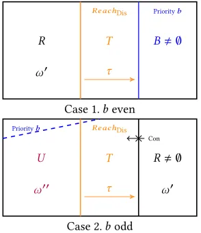
Figure 1.Strategy decompositions for Dis.
2.2 Strategy decompositions for Dis
LetW ⊆V be a subgame (i.e.a non empty induced subgraph of
V with no deadend) in which the biggest vertex priority isb. We define strategy decompositions for Dis by induction onband the size ofW. We say thatωis ab-decomposition ofWfor Dis if the following conditions hold (pictured in Figure 1).
1. Ifbis even thenω= (R,ω′),(T,τ),B
, such that: a. setsR,T, andB,∅are a partition ofW;
b. Bis the set of vertices of the top prioritybinW; c.τis a positional reachability strategy for Dis fromT toB
inW;
d.ω′is ab′-decomposition ofRfor Dis, whereb′<b. 2. Ifbis odd thenω= (U,ω′′),(T,τ),(R,ω′)
, such that: a. setsU,T, andR,∅are a partition ofW;
b. ω′is either:
i. ab′-decomposition ofRfor Dis, whereb′<b; or ii. a positional strategy for Dis that is mean-payoff winning
for her onR;
c.τis a positional reachability strategy for Dis fromT toR inW;
d.ω′′is ab′′-decomposition ofUfor Dis, whereb′′≤b; e.Ris a trap for Con inW.
We say that a subgameW has a strategy decomposition for Dis if it has ab-decomposition for someb. A heuristic, if somewhat non-standard, way to think about setsT andRin the above definition is that sets denoted byT aretransientand sets denoted byRare
recurrent. The meanings of those words here are different than in, say, Markov chains, and refer to strategic, rather than probabilistic, properties.
Given a strategy decompositionωfor Dis, we inductively define a positional strategyσ(ω)for Dis in the following way:
σ(ω)=
(
σ(ω′) ∪τ∪β ifω= (R,ω′),(T,τ),B,
σ(ω′′) ∪τ∪σ(ω′) ifω= (U,ω′′),(T,τ),(R,ω′),
whereβis an arbitrary positional strategy for Dis onB, andσ(ω′)=
ω′in case 2(b)ii.
Lemma 2.1. Ifωis a strategy decomposition ofW for Dis andW is a trap for Con, thenσ(ω)is a positional winning strategy for Dis from every vertex inW.
Proof. We proceed by induction on the number of vertices inW. The reasoning involved in the base cases (whenR=∅orU =∅) is analogous and simpler than in the inductive cases, hence we immediately proceed to the latter.
We consider two cases based on the parity of the biggest vertex prioritybinW.
First, assume thatbis even and letω = (R,ω′),(T,τ),B
be a
b-decomposition ofW. We argue that every infinite play consistent withσ(ω)is winning for Dis. If it visits vertices inBinfinitely many times then the parity condition for Dis is satisfied becausebis the biggest vertex priority and it is even. Otherwise, it must be the case that the play visits vertices inT∪Bonly finitely many times, because visiting a vertex inT always leads in finitely many steps to visiting a vertex inBby following the reachability strategyτ. Therefore, eventually the play never leavesR and is consistent with strategyσ(ω′), which is winning for Dis by the inductive hypothesis.
Next, assume thatbis odd. Letω = (U,ω′′),(T,τ),(R,ω′)
be ab-decomposition. We argue that every infinite play consistent withσ(ω)is winning for Dis. If it visitsT∪R, then by following strategyτ, it eventually reaches and never leavesR(becauseR is a trap for Con), and hence it is winning for Dis becauseσ(ω′) is a winning strategy for Dis by the inductive hypothesis, or by condition 2(b)ii. Otherwise, if such a play never visitsT∪Rthen it is winning for Dis becauseσ(ω′′)is a winning strategy for Dis by the inductive hypothesis. 2.3 Strategy decompositions for Con
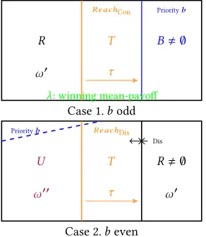
LetW ⊆V be a subgame in which the biggest vertex priority isb. We define strategy decompositions for Con by induction onband the size ofW. We say thatωis ab-decomposition ofW for Con if the following conditions hold (pictured in Figure 2).
1. Ifbis odd thenω= (R,ω′),(T,τ),B,λ
, such that: a. setsR,T, andB,∅are a partition ofW;
b. Bis the set of vertices of prioritybinW;
c.τis a positional reachability strategy for Con fromT toB inW;
d.ω′is ab′-decomposition ofRfor Con, whereb′<b; e. λis a positional strategy for Con that is mean-payoff
win-ning for him onW.
2. Ifbis even thenω= (U,ω′′),(T,τ),(R,ω′)
, such that: a. setsU,T, andR,∅are a partition ofW;
b. ω′is ab′-decomposition ofRfor Con, whereb′<b; c.τis a positional reachability strategy for Con fromT toR
inW;
d.ω′′is ab′′-decomposition ofUfor Con, whereb′′≤b; e. Ris a trap for Dis inW.
We say that a subgame has a strategy decomposition for Con if it has ab-decomposition for someb. Note that the definition is analogous to that of a strategy decomposition for Dis in most aspects, with the following differences:
• the roles of Dis and Con, and of even and odd, are swapped; • the condition 2b is simplified;
A pseudo-quasi-polynomial algorithm for mean-payoff parity games , ,
Priorityb
B,∅
ReachCon
T
τ
R
ω′
λ: winning mean-payoff
Case 1.bodd
R,∅
ω′
ReachDis
T
τ U
ω′′
Priorityb
Dis
×
[image:6.612.102.248.74.242.2]Case 2.beven
Figure 2.Strategy decompositions for Con.
Given a strategy decompositionωfor Con, we inductively define a strategyσ(ω)for Con in the following way:
• Ifb is odd andω =((R,ω′),(T,τ),B,λ), then the strategy proceeds in (possibly infinitely many) rounds. Roundi, for
i=1,2,3, . . ., involves the following steps:
1. if starting inR, followσ(ω′)for as long as staying inR; 2. if starting inT, or having arrived there fromR, followτ
untilBis reached;
3. onceBis reached, followλforn+(2n+3n+2)nCsteps and proceed to roundi+1.
• Ifbis even andω=((U,ω′′),(T,τ),(R,ω′)), then let:
σ(ω)=σ(ω′′) ∪τ∪σ(ω′).
Lemma 2.2. Ifωis a strategy decomposition ofW for Con andW is a trap for Dis, thenσ(ω)is a winning strategy for Con from every vertex inW.
Proof. We proceed by induction on the number of vertices inW, omitting the base cases (whenR=∅, orU =∅, respectively), since they are analogous and simpler than the inductive cases.
We consider two cases based on the parity ofb. First, assume thatbis even and letω = (U,ω′′),(T,τ),(R,ω′)
. Observe that a play consistent withσ(ω) = σ(ω′′) ∪τ ∪σ(ω′)either never leavesU, or if it does then after a finite number of steps (following the reachability strategyτ) it entersRand then never leaves it becauseRis a trap for Dis. It follows that the play is winning for Con by the inductive hypothesis, because it is eventually either consistent with strategyσ(ω′′)or withσ(ω′).
Next, assume thatb is odd. Letω = (R,ω′),(T,τ),B,λ
be ab-decomposition. We argue that every infinite play consistent withσ(ω)is winning for Con. If it visitsT ∪Rfinitely many times then eventually it is consistent with strategyσ(ω′)and hence it is winning for Con by the inductive hypothesis. Otherwise, it visits setBinfinitely many times and hence it satisfies the parity condi-tion for Con becausebis the highest vertex priority and it is odd. We now claim that every play consistent withσ(ω)has a negative mean payoff, and hence also satisfies the mean-payoff condition for Con. For lack of space, we do not provide a detailed and rigorous argument here, but it can be found in the full version of this pa-per [10]. The main insight, however, is that in every round, either
the strategyσ(ω′)is played for long enough to—by the inductive hypothesis—contribute a negative average cost in step 1., or the combined costs encountered in steps 1. and 2. are bounded, and hence they are eventually overwhelmed by the negative averages achieved in arbitrarily long spells of playing a mean-payoff strat-egyλ(which, by positional determinacy of mean-payoff games [11], secures mean-payoff at most−1/n) in step 3. 2.4 Existence of strategy decompositions
In the following lemma, we prove that every game can be parti-tioned into two sets of vertices, so that there is a strategy decom-position of one for Dis, and a strategy decomdecom-position of the other one for Con. Those sets correspond to the winning sets for Dis and Con, respectively.
Lemma 2.3. There is a partitionWDisandWConofV, such that
there is a strategy decomposition ofWDisfor Dis (providedWDis,∅)
and a strategy decomposition ofWConfor Con (providedWCon,∅).
The proof of Lemma 2.3 can be found in the full version of the paper [10]. It follows the usual template of using a McNaughton-Zielonka inductive argument, as adapted to mean-payoff parity games by Chatterjee et al. [7], and then simplified for threshold mean-payoff parity games by Chatterjee et al. [6, Appendix C].
Observe that Lemmas 2.1, 2.2, and 2.3 form a self-contained argument to establish both determinacy of threshold mean-payoff parity games (from every vertex, one of the players has a winning strategy), and membership of the problem of deciding the winner both in NP and in co-NP. For the latter, it suffices to note that strategy decompositions can be described in a polynomial number of bits, and it can be routinely checked in small polynomial time whether a proposed strategy decomposition for either of the players satisfies all the conditions in the corresponding definition. The NP and co-NP membership has been first established by Chatterjee and Doyen [4]; we merely give an alternative proof.
Corollary 2.4(Chatterjee and Doyen [4]). The problem of deciding the winner in mean-payoff parity games is both in NP and in co-NP.
3
Mean-payoff parity progress measures
In this section we introduce the other key concept—mean-payoff parity progress measures—that plays the critical role in achieving our main technical result—the first pseudo-quasi-polynomial algo-rithm for solving mean-payoff parity games. In Lemmas 3.1 and 3.2 we establish that mean-payoff parity progress measures witness existence of winning strategies for Dis, by providing explicit trans-lations between them and strategy decompositions for Dis.
We stress that the purpose of introducing yet another concept of witnesses for winning strategies for Dis is to shift technical focus from highlighting the recursive strategic structure of winning sets in strategy decompositions, to an order theoretic formalization that makes the recursive structure be reflected in the concept of ordered trees. The order-theoretic formalization then allows us—in Section 4—to apply the combinatorial result on succinct coding of ordered trees by Jurdziński and Lazić [19], paving the way to the pseudo-quasi-polynomial algorithm.
3.1 The definition
specific defined order) are called progressive, and an infinite path consisting only of progressive edges is winning for Dis. Then, we can derive a winning strategy for Dis if she can always follow a progressive edge and if Con has no other choice than following a progressive edge.
Recall the assumption thatd—the upper bound on the vertex priorities—is even.
Aprogress measurementis a sequence ⟨md−1,md−3, . . . ,mℓ⟩,e,
where:
• ℓis odd and 1 ≤ ℓ ≤d+1 (note that ifℓ =d+1 then ⟨md−1,md−3, . . . ,mℓ⟩is the empty sequence⟨⟩);
•mi is an element of a linearly ordered set (for simplicity, we write≤for the order relation), for each oddi, such that
ℓ≤i≤d−1;
•eis an integer such that 0≤e≤nC, ore=∞.
Aprogress labelling(µ,φ)maps vertices to progress measurements in such a way that if vertexvis mapped to
µ(v),φ(v)=
⟨md−1,md−3, . . . ,mℓ⟩,e
then
• ℓ≥π(v); and
• ife =∞thenℓis the smallest odd integer such thatℓ≥π(v). For every priorityp, 1 ≤ p ≤ d, we obtain ap-truncation ⟨md−1,md−3, . . . ,mℓ⟩|pof⟨md−1,md−3, . . . ,mℓ⟩, by removing the
components corresponding to all odd priorities smaller thanp. For example, if we fixd=8 then we have⟨a,b,c⟩|8=⟨⟩,⟨a,b,c⟩|6=
⟨a⟩, and⟨a,b,c⟩|3=⟨a,b,c⟩|2 =⟨a,b,c⟩. We compare sequences using the lexicographic order; for simplicity, and overloading no-tation, we write≤to denote it. For example, ⟨a⟩ < ⟨a,b⟩, and ⟨a,b,c⟩<⟨a,d⟩ifb<d.
Let(µ,φ)be a progress labelling. Observe that—by definition—
µ(v)|π(v) = µ(v), for every vertexv ∈ V. We say that an edge (v,u) ∈Eisprogressivein(µ,φ)if:
1. µ(v)>µ(u)|π(v); or
2. µ(v)=µ(u)|π(v),π(v)is even, andφ(v)=∞; or 3. µ(v)=µ(u),φ(v),∞, andφ(v)+c(v,u) ≥φ(u).
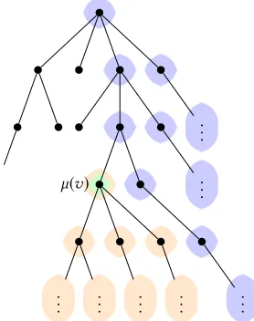
We can represent tuples as nodes in a tree where the components of the tuple represent the branching directions in the tree to go from the root to the node. For example, a tuple⟨a,b,c⟩corresponds to the node reached from the root by first reaching theath child of the root, then thebth child of this latter and finally thecth child of this one. This way, the notion of progressive edges can be seen on a tree as in Figure 3.
A progress labelling(µ,φ)is aprogress measureif:
• for every vertex owned by Dis, there is at least one outgoing edge that is progressive in(µ,φ); and
• for every vertex owned by Con, all outgoing edges are pro-gressive in(µ,φ).
In the next two sections, we prove that there is a strategy de-composition for Dis if and only is there is a progress measure.
3.2 From progress measures to strategy decompositions Lemma 3.1. If there is a progress measure then there is a strategy decomposition ofVfor Dis.
In the proof we will use the following simple fact (see, for exam-ple, Brim et al. [2]): if all the edges in an infinite path are progressive
..
. µ(v)
..
. ... ... ... ... .. . .. .
The siblings are ordered according to the linear order≤. The smallest child is on the right and the greatest on the left in the picture. An edge(v,u)is progressive if one of the three following
conditions holds:
condition 1
-µ(u)is one of the blue node,i.e.above or on the right ofµ(v).
condition 2
-π(v)is even,φ(v)=∞andµ(u)is one of the orange node,i.e.
belongs to the subtree rooted inµ(v).
condition 3
[image:7.612.370.509.74.250.2]-µ(u)=µ(v),φ(u) ∈Zandφ(v)+c(v,u) ≥φ(u).
Figure 3.Conditions for an edge to be progressive. and fulfill condition 3. of the definition, then the mean payoff of this path is non-negative (and thus winning for Dis).
Proof. We proceed by induction on the number of distinct vertex priorities in the game graph. Letb ≤dbe the highest priority appearing in the game.
The base case is whenbis the only vertex priority. Ifbis even, then by settingB=VandT =R=∅we obtain a strategy decompo-sition ofVfor Dis. Ifbis odd, then an edge can only be progressive if it satisfies condition 3. of the definition of a progressive edge; hence the progress measure yields a positional strategyω′for Dis that is mean-payoff winning for her onV. It follows that settingR=V,
T =U=∅, andω′as above, we obtain a strategy decomposition ofV for Dis.
Consider the inductive step now. First, suppose thatbis even. LetBbe the set of the vertices of priorityb. LetT be the set of vertices from which Dis has a reachability strategy toB,τbe this positional strategy and letR=V\ (B∪T). Because, by construction, there is no edge from a vertex inRowned by Dis to a vertex in
B∪T, the progress measure onVgives also a progress measure on
Rwhen restricted to its vertices. Letωbe ab′-decomposition ofR for Dis that exists by the inductive hypothesis. Note thatb′<b because the biggest priority inRis smaller thanb. It follows that
(R,ω),(T,τ),B
A pseudo-quasi-polynomial algorithm for mean-payoff parity games , ,
(If we pictured the tuples on a tree as in Figure 3, those would be the vertices that are mapped to the rightmost-top node in the tree among the nodes at least one vertex is mapped to.) LetR′be the subset ofRof those vertices having a finiteφ:{v∈R:φ(v),∞}. Suppose first thatR′,∅. An edge going out from a vertex inR′
can only be progressive if it fulfills condition 3. in the definition. It then has to go to a vertex ofR′too. Thus,R′is a trap for Con, and Dis has a winning strategyω′inR′for the mean-payoff game.
LetTbe the set of vertices from which Dis has a strategy to reach
R′and letτthis positional reachability strategy. LetU =V\ (R′∪
T). Because, by construction, there is no edge from a vertex inU owned by Dis to a vertex inR′∪T, then the progress measure onV gives also a progress measure onUwhen restricted to its vertices. We can then apply the inductive hypothesis and getωa strategy decomposition ofUfor Dis. Note that (U,ω),(T,τ),(R′,ω′)
is a strategy decomposition ofV for Dis.
Suppose now thatR′=∅. The non-empty setRcontains only verticesvsuch thatφ(v)=∞. Then, by definition and because all those vertices are associated with the same tuple, they must all have priorityb′orb′+1 for some even numberb′.
Any edge going out from a vertex ofRis progressive if and only if it fulfills condition 2. of the definition. Thus, the priority of all the vertices inRhas to be even and is consequentlyb′withb′<b. LetR′′={u∈V:µ(v)=µ(u)|π(v)forv∈R}. (If we picture the
tuples on a tree as in Figure 3, those are the vertices that are mapped to the nodes in the subtree rooted in the node corresponding toR.) By definition, the priority of all those vertices is also smaller thanb. Moreover, an edge going out from a vertex inR′′can only be pro-gressive if it goes to a vertex inR′′too. So,R′′is a trap for Con and an edge from a vertex inR′′owned by Dis to a vertex not inR′′ cannot be progressive. So the progress measure onV gives also a progress measure onR′′when restricted to its vertices. By the inductive hypothesis, there is a strategy decompositionω′′ofR′′ for Dis. LetT be the set of vertices from which Dis has a strategy to reachR′′and letτbe a corresponding positional reachability strat-egy. LetU=V\ (R′′∪T). Because, by construction, there is no edge inUfrom a vertex owned by Dis to a vertex inR′′∪T, the progress measure onVgives also a progress measure onUwhen restricted to its vertices. By the inductive hypothesis, there is a strategy de-compositionωofUfor Dis. Note that (U,ω),(T,τ),(R′′,ω′′)
is a strategy decomposition ofV for Dis. 3.3 From strategy decompositions to progress measures Lemma 3.2. If there is a strategy decomposition ofV for Dis then there is a progress measure.
Proof. The proof is by induction on the size of the game graph. Let
bbe the biggest vertex priority inV. We strengthen the inductive hypothesis by requiring that the progress measure(µ,φ)whose existence is claimed in the lemma is such that all sequences in the image ofµhave the same prefix corresponding to indicesk, such thatk>b. We need to consider two cases based on the parity ofb.
Suppose first thatbis even. Letω = (R,ω′),(T,τ),B
be ab -decomposition ofVfor Dis. SinceB,∅, by the inductive hypothesis
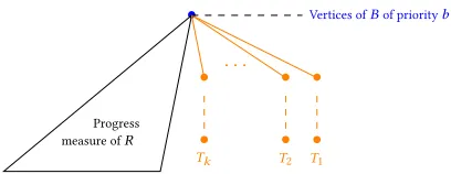
there is a progress measure(µ′,φ′)onR. For every vertexv ∈T, define itsτ-distance toBto be the largest number of edges on a path starting atv, consistent withτ, and whose only vertex inBis the last one. Letkbe the largest suchτ-distance, and we defineTi, 1≤i≤k, to be the set of vertices inTwhoseτ-distance toBisi.
•
Progress measure ofR
• •
. . .
•
Vertices ofBof priorityb
• T1
• T2
[image:8.612.334.538.77.156.2]• Tk
Figure 4.Construction of a progress measure -beven (the common prefix is not pictured).
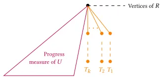
Let⟨md−1,md−3, . . . ,mb+1⟩ be the common prefix of all se-quences in the image ofµ′. Lett1,t2, . . . ,tk be elements of the linearly ordered set used in progress measurements, such that for everyr that is the component of a sequence in the image ofµ′ corresponding to priorityb−1, we haver >tk >· · · >t2 >t1, and lettbe a chosen element of the linearly ordered set (it does not matter which one). Define the progress labelling(µ,φ)for all verticesv∈V as follows:
µ(v),φ(v)
=
µ′(v),φ′(v)
ifv∈R, ⟨md−1, . . . ,mb+1,ti,mb−3, . . . ,mℓ⟩,∞
ifv∈Ti,1≤i≤k, ⟨md−1,md−3, . . . ,mb+1⟩,∞
ifv∈B; whereℓ is the smallest odd number no smaller thanπ(v)and
mb−3=. . .=mℓ=t.
The progress labelling(µ,φ)as defined above is a desired progress measure. It is illustrated as a tree in Figure 4.
Suppose now thatbis odd. Letω = (U,ω′′),(T,τ),(R,ω′)
be ab-decomposition ofV for Dis. Defineτ-distances, setsTi, and elementstiandtfor 1≤i≤k, in the analogous way to the “evenb” case, replacing setBby setR. By the inductive hypothesis, there is a progress measure(µ′′,φ′′)onU, and let⟨md−1,md−3, . . . ,mb+2⟩
be the common prefix of all sequences in the image ofµ′′. We define a progress labelling(µ,φ)for all vertices inU∪T as follows:
µ(v),φ(v)=
µ′′(v),φ′′(v)
ifv∈U, ⟨md−1, . . . ,mb+2,ti,mb−3, . . . ,mℓ⟩,∞
ifv ∈Ti, 1≤i≤k; whereℓ is the smallest odd number no smaller thanπ(v)and
mb−3=. . .=mℓ=t.
Ifω′is ab′-decomposition ofRforb′<b(case 2(b)i), then by the inductive hypothesis, there is a progress measure(µ′,φ′)onR. Without loss of generality, assume that all sequences in the images ofµ′and ofµ′′have the common prefix⟨md−1,md−3, . . . ,mb+2⟩,
and that for alluandrthat are the components of a sequence in the images ofµ′′andµ′, respectively, corresponding to priorityb, we haveu >tk >tk−1>· · ·>t1 >r. Define the progress labelling
(µ,φ)for all verticesv ∈Rin the following way:
µ(v),φ(v)
= µ′(v),φ′(v)
.
This is illustrated in Figure 5.
If, instead,ω′is a positional strategy for Dis that is mean-payoff winning for him onR(case 2(b)ii), then by the result of Brim et al. [2], there is an energy progress measurebφfor Dis onR. Letr
′
•
Progress measure ofU
• •
. . .
•
• T1
• T2
• Tk
•
[image:9.612.72.274.78.156.2]Progress measure ofR
Figure 5.Construction of a progress measure -bodd - case 2(b)i. •
Progress measure ofU
• •
. . .
•
• T1
• T2
• Tk
Vertices ofR
Figure 6.Construction of a progress measure - case 2(b)ii.
verticesv∈Rin the following way:
µ(v),φ(v)=
⟨md−1,md−3, . . . ,mb+2,r′⟩,
b
φ(v).
This is illustrated in Figure 6.
The progress labelling(µ,φ)as defined above is a desired progress
measure.
4
Computing progress measures by lifting
In this section, we give a so-called lifting algorithm which identifies the winning sets for Dis and for Con by computing a progress measure on the winning set for Dis.
By thetreeof a progress labelling(µ,φ), we mean the ordered tree whose nodes are all prefixes of all sequencesµ(v)asvranges over the vertices of the game graph, and such that every vertexvlabels the nodeµ(v)of the tree. Let us say that progress labellings(µ,φ) and(µ′,φ′)areisomorphicif and only if their (partially labelled ordered) trees are isomorphic andφ=φ′.
We shall work with the following ordering on finite binary strings:
0s<ε, ε<1s, bs<bs′if and only ifs<s′, whereεdenotes the empty string,branges over binary digits, and
s,s′range over binary strings.
Recall thatnis the number of vertices, andd(assumed even) is the number of priorities.
LetSn,dbe all sequences⟨md−1,md−3, . . . ,mℓ⟩of binary strings such that:
• ℓis odd and 1≤ℓ≤d+1; • Íd−1
i=ℓ |mi| ≤ ⌈lgn⌉;
and let us call a progress measurement, labelling or measuresuccinct
if and only if all the sequences⟨md−1,md−3, . . . ,mℓ⟩involved are members ofSn,d.
Lemma 4.1. For every progress labelling, there exists a succinct isomorphic one.
Proof. This is an immediate consequence of [19, Lemma 1], since for every progress labelling, its tree is of height at mostd/2 and
has at mostnleaves.
Corollary 4.2. Lemmas 3.1 and 3.2 hold when restricted to succinct progress measures.
We now order progress measurements lexicographically: ⟨md−1,md−3, . . . ,mℓ⟩,e
<
⟨md′−
1,m
′
d−3, . . . ,m
′ ℓ′⟩,e′
if and only if either⟨md−1,md−3, . . . ,mℓ⟩<⟨md′−
1,m
′
d−3, . . . ,m
′ ℓ′⟩,
or⟨md−1,md−3, . . . ,mℓ⟩=⟨md′−
1,m
′
d−3, . . . ,m
′
ℓ′⟩ande<e′
and we extend them by a new greatest progress measurement (⊤,∞). We then revise the set of progress labellings to allow the extended progress measurements, and we (partially) order it point-wise:
(µ,φ) ≤ (µ′,φ′)if and only if,
for allv∈V, µ(v),φ(v)≤ µ′(v),φ(v′).
We also revise the definition of a progress measure by stipulating that an edge(v,u)which involves the progress measurement(⊤,∞) is progressive if and only if the progress measurement ofvis(⊤,∞). For any succinct progress labelling(µ,φ)and edge(v,u), we set lift(µ,φ,v,u)to be the minimum succinct progress measurement ⟨md−1,md−3, . . . ,mℓ⟩,ewhich is at least µ(v),φ(v)and such
that(v,u)is progressive in the updated succinct progress labelling
µ
v7→ ⟨md−1,md−3, . . . ,mℓ⟩
,φ[v7→e].
For any vertexv, we define an operator Liftvon succinct progress labellings as follows:
Liftv(µ,φ)(w)=
µ(w),φ(w)
ifw,v,
min(v,u)∈Elift(µ,φ,v,u) if Dis ownsw=v,
max(v,u)∈Elift(µ,φ,v,u) if Con ownsw=v. Theorem 4.3(Correctness of lifting algorithm).
1. The set of all succinct progress labellings ordered pointwise is a complete lattice.
2. Each operatorLiftvis inflationary and monotone.
3. From every succinct progress labelling(µ,φ), every sequence of applications of operatorsLiftveventually reaches the least simultaneous fixed point of allLiftv that is greater than or equal to(µ,φ).
4. A succinct progress labelling(µ,φ)is a simultaneous fixed point of all operatorsLiftvif and only if it is a succinct progress measure.
5. If(µ∗,φ∗)is the least succinct progress measure, then{v :
µ∗(v),φ∗(v)
,(⊤,∞)}is the set of winning positions for
Dis.
Proof. 1. The partial order of all succinct progress labellings is the pointwise product ofncopies of the finite linear order of all succinct progress measurements.
2. We have inflation, i.e. Liftv(µ,φ)(w) ≥ µ(w),φ(w)
, by the definitions of Liftv(µ,φ)(w)and lift(µ,φ,v,u).
[image:9.612.90.252.204.282.2]A pseudo-quasi-polynomial algorithm for mean-payoff parity games , ,
1. Initialise(µ,φ)to the least succinct progress labelling (v7→ ⟨⟩,v7→0)
2. While Liftv(µ,φ),(µ,φ)for somev, update(µ,φ)to become Liftv(µ,φ).
3. Return the setWDis={v : µ(v),φ(v),(⊤,∞)}of
winning positions for Dis.
Table 1.The lifting algorithm.
lift(µ′,φ′,v,u), which is in turn implied by the straightfor-ward observation that, whenever an edge is progressive with respect to a progress labelling, it remains progressive af-ter any lessening of the progress measurement of its target vertex.
3. This holds for any family of inflationary monotone opera-tors on a finite complete lattice. Consider any such maxi-mal sequence from(µ,φ). It is an upward chain from(µ,φ) to some(µ∗,φ∗)which is a simultaneous fixed point of all the operators. For any(µ′,φ′) ≥ (µ,φ)which is also a si-multaneous fixed point, a simple induction confirms that (µ∗,φ∗) ≤ (µ′,φ′).
4. Here we have a rewording of the definition of a succinct progress measure.
5. LetW = {v : µ∗(v),φ∗(v)
, (⊤,∞)}. The set of
win-ning positions for Dis is contained inW by Lemma 2.3, Lemma 3.2 and Corollary 4.2, because(µ∗,φ∗)is the least succinct progress measure.
Since(µ∗,φ∗)is a progress measure, we have that, for ev-ery progressive edge(v,u), if µ∗(v),φ∗(v)
,(⊤,∞)then
µ∗(u),φ∗(u)
,(⊤,∞). In order to show that Dis has a
win-ning strategy from every vertex inW, it remains to apply Lemmas 3.1 and 2.1 to the subgame consisting of the vertices inW.
Lemma 4.4(Jurdziński and Lazić [19]). Depending on the asymp-totic growth ofdas a function ofn, the size of the setSn,d is as follows:
1.On1+o(1)ifd=o(logn); 2. Θnlg(δ+1)+lg(eδ)+1.p
lognifd/2=⌈δlgn⌉, for some pos-itive constantδ, and whereeδ =(1+1/δ)δ;
3.Odnlg(d/lgn)+lge+o(1)ifd=ω(logn).
Theorem 4.5(Complexity of lifting algorithm). Depending on the asymptotic growth ofdas a function ofn, the running time of the algorithm is as follows:
1.Omn2+o(1)Cifd=o(logn); 2.O
mnlg(δ+1)+lg(eδ)+2C·logd·p
logn
ifd ≤2⌈δlgn⌉, for some positive constantδ;
3.O
dmnlg(d/lgn)+2.45Cifd=ω(logη).
The algorithm works in spaceO(n·logn·logd).
Proof. The work space requirement is dominated by the number of bits needed to store a single succinct progress labelling, which is at mostn(⌈lgn⌉ ⌈lgd⌉+⌈lg(nC)⌉).
Since bounded-depth successors of elements ofSn,d are com-putable in timeO(logn·logd)(cf. the proof of [19, Theorem 7], the Liftvoperators can be implemented to work in timeO(deg(v) · (logn·logd+logC)). It then follows, observing that the algorithm lifts each vertex at most|Sn,d|(nC+1)times, that its running time is bounded by
O Õ
v∈V
deg(v) · (logn·logd+logC)|Sn,d|(nC+1)
!
=
O mnC(logn·logd+logC)|Sn,d| .
From there, the various stated bounds are obtained by applying Lemma 4.4, and by suppressing some of the multiplicative factors that are logarithmic in the bit-size of the input. Suppressing the logCfactor is justified by using the unit-cost RAM model, which is the industry standard in algorithm analysis. The reasons for suppressing the lognand logdfactors are more varied: in case 1, they are absorbed by theo(1)term in the exponent ofn, and in case 3, they are absorbed in the 2.45 term in the exponent ofn, because lge<1.4427.
5
From winning sets to strategy
decompositions for Con
The pseudo-quasi-polynomial lifting algorithm computes the least progress measure and hence, by Lemmas 3.1 and 2.1, it can be easily adapted to synthesize a winning strategy for Dis from all vertices in her winning set. In this section we tackle the problem of strategy synthesis for Con. By (the proof of) Lemma 2.2, in order to synthesize a winning strategy for Con, it suffices to compute a strategy decomposition for him. We argue that this can also be achieved in pseudo-quasi-polynomial time.
Theorem 5.1(Complexity of computing strategy decompositions).
There is a pseudo-quasi-polynomial algorithm that computes strategy decompositions for both players on their winning sets.
In order to establish that strategy decompositions for Con can be computed in pseudo-quasi-polynomial time, it suffices to prove the following lemma, because the polynomial-time oracle algorithm becomes a pseudo-quasi-polynomial algorithm, once the oracle for computing winning strategies in mean-payoff games is replaced by a pseudo-polynomial algorithm [2, 8, 25], and the oracle for computing the winning sets in mean-payoff parity games is replaced by the pseudo-quasi-polynomial procedure from Section 4.
Lemma 5.2. There is a polynomial-time algorithm, with oracles for computing winning strategies in mean-payoff games and for com-puting winning sets in mean-payoff parity games, that computes a strategy decomposition for Con of his winning set.
Proof. Without loss of generality, we may assume that Con has a winning strategy from every vertex inV, since a single call to the oracle allows us to reduceVto the subgame corresponding to the winning set for Con.
with the description of the recursive procedure, we elaborate an in-ductive proof that it does indeed compute a strategy decomposition for Con onV.
Note that our procedure avoids incurring the penalty of adding to its running time a factor that is exponential in the number of distinct vertex priorities, by repeatedly using the oracle for computing the winning sets in appropriately chosen subgames. We give a detailed analysis of the worst-case running time at the end of this proof.
LetBbe the set of vertices of the highest priorityb; letT be the set of vertices (not including vertices inB) from which Dis has a strategy to reach a vertex inB; letτbe a corresponding positional rechability strategy; and letR=V\ (B∪T). We consider two cases, depending on the parity ofb.
Evenb.Call the oracle to obtain the partitionRConandRDisofR,
the winning sets for Con and for Dis, respectively, in the subgameR. We argue thatRCon , ∅. Otherwise, by Lemma 2.3, there is a
strategy decompositionωofRfor Dis, and hence (R,ω),(T,τ),B
is a strategy decomposition ofV for Dis, which, by Lemma 2.1, contradicts the assumption that Con has a winning strategy from every vertex.
LetT′be the set of vertices (not including vertices inRCon)
from which Con has a strategy to reach a vertex inRCon, and
letτ′be a corresponding positional reachability strategy, and let
U =V\ (RCon∪T′). By the inductive hypothesis, a recursive call of our procedure onRConwill produce a strategy decompositionω′
ofRConfor Con, and another recursive call of the procedure onU
will produce a strategy decompositionω′′ofUfor Con. We claim that (U,ω′′),(T′,τ′),(RCon,ω′)
is a strategy decomposition ofV for Con.
Oddb. Call the oracle for computing positional winning strategies in mean-payoff games to obtain a positional strategyλfor Con that is mean-payoff winning for him onV; such a strategy exists because Con has a mean-payoff parity winning strategy from every vertex. SinceRis a trap for Con, it must be the case that Con has a winning strategy from every vertex in the subgameR. By the inductive hypothesis, a recursive call of our procedure onRwill produce a strategy decompositionω′ofRfor Con. We claim that
(R,ω′),(T,τ),B,λ
is a strategy decomposition ofV for Con. It remains to argue that the recursive procedure described above works in polynomial time in the worst case. Observe that in both cases considered above, a call of the procedure on a game results in two or one recursive calls, respectively. In both cases, the re-cursive calls are applied to subgames with strictly fewer vertices, and—crucially for the complexity analysis—in the former case, the two recursive calls are applied to subgames on disjoint sets of ver-tices. Additional work (other than recursive calls and oracle calls) in both cases can be bounded byO(m), since the time needed is dominated by the worst case bound on the computation of reach-ability strategies. Overall, the running time functionT(n)of the recursive procedure, wherenis the number of vertices in the input game graph, satisfies the following recurrence:
T(n) ≤T(n′)+T(n′′)+O(m), wheren′+n′′<n, and henceT(n)=O(nm).
6
Conclusion
Our main result is the first pseudo-quasi-polynomial algorithm for computing the values of mean-payoff parity games, and hence also for deciding the winner in energy parity games and in parity games with weights. The main technical tools that we introduce to achieve the main result are strategy decompositions and progress measures for the threshold version of mean-payoff games. We believe that our techniques can be adapted to also produce optimal strategies for both players (i.e., the strategies that secure the value that we show how to compute). Another direction for future work is improving the complexity of solving stochastic mean-payoff parity games [5].
Acknowledgements
This research has been supported by the EPSRC grant EP/P020992/1 (Solving Parity Games in Theory and Practice).
References
[1] P. Bouyer, N. Markey, J. Olschewski, and M. Ummels. 2011. Measuring permis-siveness in parity games: Mean-payoff parity games revisited. InATVA. 135–149. [2] L. Brim, J. Chaloupka, L. Doyen, R. Gentilini, and J.-F. Raskin. 2011. Faster algorithms for mean-payoff games.Form. Methods Syst. Des.38, 2 (2011), 97–118. [3] C. S. Calude, S. Jain, B. Khoussainov, W. Li, and F. Stephan. 2017. Deciding parity
games in quasipolynomial time. InSTOC. 252–263.
[4] K. Chatterjee and L. Doyen. 2012. Energy parity games.Theoretical Computer Science458 (2012), 49–60.
[5] K. Chatterjee, L. Doyen, H. Gimbert, and Y. Oualhadj. 2014. Perfect-information stochastic mean-payoff parity games. InFOSSACS. 210–225.
[6] K. Chatterjee, M. Henzinger, and A. Svozil. 2017. Faster algorithms for mean-payoff parity games. InMFCS. 39:1–39:17.
[7] K. Chatterjee, T. A. Henzinger, and M. Jurdziński. 2005. Mean-payoff parity games. InLICS. 178–187.
[8] C. Comin and R. Rizzi. 2017. Improved pseudo-polynomial bound for the value problem and optimal strategy synthesis in mean payoff games.Algorithmica77, 4 (2017), 995–1021.
[9] A. Condon. 1992. The complexity of stochastic games.Information and Compu-tation96, 2 (1992), 203–224.
[10] L. Daviaud, M. Jurdziński, and M. Lazić. 2018. A pseudo-quasi-polynomial algo-rithm for solving mean-payoff parity games. arXiv:1803.04756. (2018). [11] A. Ehrenfeucht and J. Mycielski. 1979. Positional strategies for mean payoff
games.Journal of Game Theory8, 2 (1979), 109–113.
[12] E. A. Emerson and C. Jutla. 1991. Tree automata, mu-calculus and determinacy. InFOCS. 368–377.
[13] E. A. Emerson, C. Jutla, and A. P. Sistla. 2001. On model-checking for fragments ofµ-calculus.Theoretical Computer Science258, 1–2 (2001), 491–522. [14] J. Fearnley, S. Jain, S. Schewe, F. Stephan, and D. Wojtczak. 2017. An ordered
approach to solving parity games in quasi polynomial time and quasi linear space. InSPIN. 112–121.
[15] N. Fijalkow and M. Zimmermann. 2014. Parity and Streett games with costs.
Logical Methods in Computer Science10, 1:14 (2014), 1–29.
[16] Y. Gurevich and L. Harrington. 1982. Trees, automata, and games. InSTOC. 60–65.
[17] D. S. Johnson. 2007. The NP-completeness column: Finding needles in haystacks.
ACM Transactions on Algorithms3, 2 (2007).
[18] M. Jurdziński. 2000. Small progress measures for solving parity games. InSTACS. 290–301.
[19] M. Jurdziński and R. Lazić. 2017. Succinct progress measures for solving parity games. InLICS. 1–9.
[20] N. Klarlund and D. Kozen. 1995. Rabin measures.Chicago Journal of Theoretical Computer Science(1995). Article 3.
[21] R. McNaughton. 1993. Infinite games played on finite graphs.Annals of Pure and Applied Logic65, 2 (1993), 149–184.
[22] S. Schewe, A. Weinert, and M. Ziemmermann. 2018. Parity games with weights. arXiv:1804.06168. (2018).
[23] W. Thomas. 1995. On the synthesis of strategies in infinite games. InSTACS. 1–13.
[24] W. Zielonka. 1998. Infinite games on finitely coloured graphs with applications to automata on infinite trees.Theoretical Computer Science200 (1998), 135–183. [25] U. Zwick and M. Paterson. 1996. The complexity of mean-payoff games on graphs.