City, University of London Institutional Repository
Citation
:
Karabağ, C., Verhoeven, J. ORCID: 0000-0002-0738-8517, Miller, N. and
Reyes-Aldasoro, C. C. ORCID: 0000-0002-9466-2018 (2019). Texture Segmentation: An
Objective Comparison between Five Traditional Algorithms and a Deep-Learning U-Net
Architecture. Applied Sciences, 9, 3900.. doi: 10.3390/app9183900
This is the published version of the paper.
This version of the publication may differ from the final published
version.
Permanent repository link:
http://openaccess.city.ac.uk/id/eprint/22853/
Link to published version
:
http://dx.doi.org/10.3390/app9183900
Copyright and reuse:
City Research Online aims to make research
outputs of City, University of London available to a wider audience.
Copyright and Moral Rights remain with the author(s) and/or copyright
holders. URLs from City Research Online may be freely distributed and
linked to.
sciences
Article
Texture Segmentation: An Objective Comparison
between Five Traditional Algorithms and a
Deep-Learning U-Net Architecture
Cefa Karaba˘g1, Jo Verhoeven2,3, Naomi Rachel Miller2and Constantino Carlos Reyes-Aldasoro1,*
1 Department of Electrical and Electronic Engineering, Research Centre for Biomedical Engineering,
School of Mathematics, Computer Science and Engineering, City, University of London, London EC1V 0HB, UK; [email protected]
2 School of Health Sciences, Division of Language & Communication Science, Phonetics Laboratory,
University of London, London EC1R 1UW, UK; [email protected] or [email protected] (J.V.); [email protected] (N.R.M.)
3 Department of Linguistics CLIPS, University of Antwerp, 2000 Antwerp, Belgium
* Correspondence: [email protected]
Received: 30 July 2019; Accepted: 10 September 2019; Published: 17 September 2019
Abstract: This paper compares a series of traditional and deep learning methodologies for the segmentation of textures. Six well-known texture composites first published by Randen and Husøy were used to compare traditional segmentation techniques (co-occurrence, filtering, local binary patterns, watershed, multiresolution sub-band filtering) against a deep-learning approach based on the U-Net architecture. For the latter, the effects of depth of the network, number of epochs and different optimisation algorithms were investigated. Overall, the best results were provided by the deep-learning approach. However, the best results were distributed within the parameters, and many configurations provided results well below the traditional techniques.
Keywords:texture; segmentation; deep learning
1. Introduction
Texture, and more specifically textural characteristics in images, has been widely studied in the past decades as texture is one of the most important features present in images and can be used for feature extraction [1–8] and classification and segmentation [9–14]. The areas of study where texture is present range from crystallographic texture [15], stratigraphy [16,17], food science of potatoes [18] or apples [19], patterned fabrics [20] to natural stone industry [21]. In medical imaging, there is a large volume of research which exploits the use of texture for different purposes, like segmentation or classification in most acquisition modalities like magnetic resonance imaging (MRI) [22–26], ultrasound [27,28], computed tomography (CT) [29–31], microscopy [32,33] and histology [34]. There are numerous approaches to texture: Haralick’s co-occurrence matrix [4,5] on the spatial domain, Gabor filters [35–37] and ordered pyramids [8] on the spectral domain, wavelets [38,39] or Markov random fields [3,40].
In recent years, advances in artificial intelligence have revolutionised image processing tasks. Several deep learning approaches [41–43] have achieved outstanding results in difficult tasks such as those of the ImageNet Large Scale Visual Recognition Challenge (ILSVRC) [44]. Convolutional Neural Networks (CNNs) are well suited to analyse textures as their repetitive patterns can be learned and identified by filter banks [45]. The U-Net architecture proposed by Ronneberger [46] has become a very widely used tool for segmentation and analysis reaching thousands of citations in the few years since it was published. U-Nets have been used widely, for instance, for road extraction [47], singing voice
separation [48], automatic brain tumour detection and segmentation [49] and cell counting, detection, and morphometry [50]. The success of these deep learning approaches in very different areas invites for their application on texture analysis.
In this work, a U-Net architecture for the segmentation of textures is implemented and objectively compared against several popular traditional segmentation strategies. The traditional algorithms (co-occurrence matrices [5], watershed [51], local binary patterns (LBP) [52,53], filtering [54] and multiresolution sub-band filtering (MSBF) [8]) were selected as these have been previously published using the texture composites proposed by Randen [55] and thus an objective numerical comparison is possible.
To perform an objective comparison, six well-known texture composites from the Brodatz [56] album, first published by Randen and Husøy [54], are segmented with U-Nets of different configurations and parameters and the results compared against previously published results. The effects of the configuration of the networks, namely, number of epochs, depth of the network in the number of layers, and type of optimisation algorithm are assessed. All the programming was performed in MatlabR (The MathworksTM, Natick, MA, USA) and the code is freely available through
GitHub (https://github.com/reyesaldasoro/Texture-Segmentation). 2. Materials and Methods
2.1. Texture Composite Images
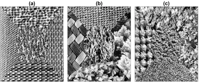
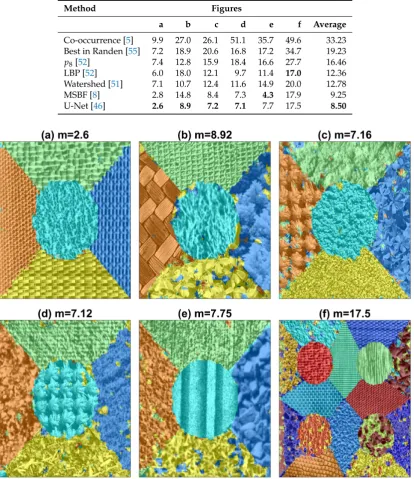
Six composite texture images were segmented in this work (Figure1). The first five composites are images of 256×256 pixels and consist of five different textures whilst the last one is 512×512 pixels and is formed with 16 different textures. The masks with which these were formed are shown in Figure2. It should be highlighted that these textures have been histogram equalised prior to the arrangement and thus they cannot be distinguished by the general intensity of each region. It is frequent that comparisons are made over textures that are not equalised (e.g., [57] Figure 3, [45] Figure 2) and thus the segmentation is not only based on the texture but the average intensity of the regions. Furthermore, whilst some textures are easy to distinguish, there are some that are quite challenging, for instance, the difference between the central and bottom regions in Figure1c or the top left corners of Figure1d,e.
[image:3.595.89.508.506.682.2]Appl. Sci.2019,xx, 5 3 of 15
Figure 1. Six composite texture images. (a-e) Texture arrangements with five textures. (f) Texture arrangement with sixteen textures. Notice first, that individual textures have been histogram equalised and thus each region cannot be distinguished by the intensity, and second, some textures area easier to distinguish (e.g., (a)) than others (e.g., (d)).
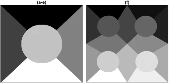
Figure 2.(a) Mask corresponding to texture arrangements of Figs.1(a-e). (b) Mask corresponding to texture arrangements of Figure1(f).
2.2. Training data
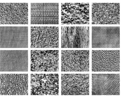
The training data in [54] is provided separately and is shown in Figure 3 for the first five composites and in Figure4for the last case. For the purpose of training the U-Nets, the training images were tessellated into sub-regions of 32×32 pixels each.
Appl. Sci.2019,9, 3900 3 of 14
Figure 1. Six composite texture images. (a-e) Texture arrangements with five textures. (f) Texture arrangement with sixteen textures. Notice first, that individual textures have been histogram equalised and thus each region cannot be distinguished by the intensity, and second, some textures area easier to distinguish (e.g., (a)) than others (e.g., (d)).
Figure 2.(a) Mask corresponding to texture arrangements of Figs.1(a-e). (b) Mask corresponding to texture arrangements of Figure1(f).
2.2. Training data
[image:4.595.158.438.332.472.2]The training data in [54] is provided separately and is shown in Figure 3 for the first five composites and in Figure4for the last case. For the purpose of training the U-Nets, the training images were tessellated into sub-regions of 32×32 pixels each.
Figure 1. Six composite texture images. (a–e) Texture arrangements with five textures. (f) Texture arrangement with sixteen textures. Notice first, that individual textures have been histogram equalised and thus each region cannot be distinguished by the intensity, and second, some textures are easier to distinguish (e.g., (a)) than others (e.g., (d)).
Figure 2. (Left) Mask corresponding to texture arrangements of Figure 1a–e. (Right) Mask corresponding to texture arrangements of Figure1f.
2.2. Training Data
The training data in [54] is provided separately and is shown in Figure 3 for the first five composites and in Figure4for the last case. For the purpose of training the U-Nets, the training images were tessellated into sub-regions of 32×32 pixels each.
Figure 3.Training images corresponding to the texture arrangements of Figure1a–e.
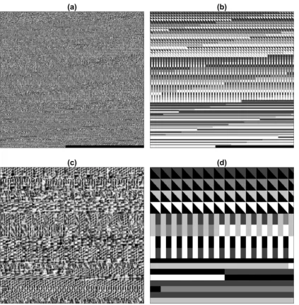
[image:5.595.103.495.429.739.2]Figure 5.Montages of the texture pairs created to train the deep learning networks. Training images shown in Figures3and4were tessellated and arranged in diagonal, vertical and horizontal pairs. (a) Texture pairs. (b) Labels. (c) Detail of the texture pairs. (d) Detail of the labels.
2.3. Traditional Texture Segmentation Algorithms
For this paper, we compared the results of the following texture segmentation algorithms: co-occurrence matrices [5], watershed [51], local binary patterns (LBP) [52,53], filtering [54] and multiresolution sub-band filtering (MSBF) [8] against a U-Net architecture [46].
The traditional algorithms have been thoroughly described in the literature; however, for completeness, a short explanation of how features are extracted with each algorithm will follow. For a discussion of traditional texture techniques, the reader is referred to any of the following reviews [58–60].
and directionality. For example, in coarse images, the grey level of the pixels change slightly with distance, while for fine textures the levels change rapidly. From this matrix, different features like entropy, uniformity, maximum probability, contrast, difference moment, inverse difference moment and correlation can be calculated [5]. Once the features have been calculated, classifiers can be applied directly, or further processing like the watershed transforms can be applied.
Watershed transforms are based on a topographical analogy of a landscape. Should water fall in this landscape, it would find the path through which it could reach a region of minimum altitude, i.e., a basin, sometimes called lake or sea. For each point in the landscape (or pixel of the image) there is a path towards one and only one basin. Thus, the landscape can be partitioned into catchment basins or regions of influence of the regional minima and the boundaries between the basins (e.g., points of inflection) are called the watershed lines. [61]. The watershed transform can be applied to features extracted from the co-occurrence matrix [51]. The basins produced can further be iteratively merged to segment textured regions.
Local binary patterns (LBP) [52], explore the relations between neighbouring pixels. These methods concentrate on the relative intensity relations between the pixels in a small neighbourhood and not in their absolute intensity values or the spatial relationship of the whole data. The underneath assumption is that texture is not properly described by the Fourier spectrum and traditional frequency filters. The texture analysis is based on the relationship of the pixels of a 3×3 neighbourhood. A Texture Unit is first calculated by differentiating the grey level of a central pixel with the grey level of its neighbours. The difference is measured if the neighbour is greater or lower than the central pixel. Two advantages of LBP is that there is no need of quantising images and there is a certain immunity to low frequency artefacts. In a more recent paper, Ojala [53] presented another variation to the LBP by considering the sign of the difference of the grey-level differences histograms. Under the new consideration, LBP is a particular case of the new operator calledp8. This operator
is considered as a probability distribution of grey levels, whenp(g0,g1)denotes the co-occurrence
probabilities, they usep(g0,g1−g0)as a joint distribution.
Filtering, in the context of image processing, consists of a process that will modify the pixel values. There are spatial filters, which are applied directly to the values of the images (e.g., average neighbouring pixels to blur an image) and filters which are applied after a transformation of the data has been performed. Thus a filter in the frequency or Fourier domain will be applied after the image has been converted through the Fourier transform. The filters in the Fourier domain are sometimes named after the frequencies that are to be allowed to pass through them: low pass, band pass and high pass filters. Since textures can vary in their spectral distribution in the frequency domain, a set of sub-band filters can help in their discrimination. One common frequency filtering approach is that of Gabor multichannel filter banks [2,10,62–64].
The partitioning of the Fourier space can be achieved in different ways, Gabor being only one. A multiresolution approach, based on finite prolate spheroidal sequences is described in [8]. The Fourier space is divided into frequencies and orientations, which are further subdivided in a multiresolution approach. Each filter then produces a feature; different textures are captured by different filters. In addition, a feature selection strategy can improve the texture segmentation.
2.4. U-Net Configuration
The basic U-Net architecture was formed with the following layers:Input, Convolutional, ReLu, Max Pooling, Transposed Convolutional, Convolutional, SoftmaxandPixel Classification. Two levels of depth were investigated by repeating the downsampling and upsampling blocks in the following configurations:
15 layers: Input,
Convolutional, ReLu, Max Pooling, Convolutional, ReLu,
Transposed Convolutional, Convolutional, Transposed Convolutional, Convolutional, Softmax,
Pixel Classification
20 layers: Input,
Convolutional, ReLu, Max Pooling, Convolutional, ReLu, Max Pooling, Convolutional, ReLu, Max Pooling, Convolutional, ReLu,
Transposed Convolutional, Convolutional, Transposed Convolutional, Convolutional, Transposed Convolutional, Convolutional, Softmax,
Pixel Classification.
The image input layer was configured for the 32×32 patches. The convolutional layers consisted of 64 filters of size 3 and padding of 1. The pooling size was 2 with stride of 2. The transposed convolutional had a filter size of 4, stride of 2 and cropping of 1. The numbers of epochs evaluated were 10, 20, 50, 100. The following optimisation algorithms were analysed: stochastic gradient descent (sgdm), Adam (Adam) [65] and Root Mean Square Propagation (RMSprop). One last investigation was performed by training the 20 layer network two separate times to investigate the variability of the process.
2.5. Misclassification
For the purposes of assessing the algorithms, a pixel-based assessment will be considered. Each pixel whose class is correctly determined by the segmentation algorithm will be counted as Correct, every pixel which the algorithm assigns a different class will be considered asIncorrect. Notice that since there is no foreground/background distinction but rather correct or incorrect, both True Positive(TP) andTrue Negative(TN) are included as correct, andFalse Positive(FP) andFalse Negative(FN) are included in the incorrect. Thus, themisclassificationin percentage, or classification error, will be calculated as number of incorrect pixels divided by the total number of pixels of the image
m = 100∗(FP+FN)/(TP+TN+FP+FN). The accuracy can be calculated as the complement
a=100∗(TP+TN)/(TP+TN+FP+FN).
3. Results
For each image, the networks were trained with the 3 different optimisation algorithms, 3 layer configurations and 4 epoch numbers, for a total of 36 different combinations. Thus for the 6 composite images there were 216 results. The misclassification of each segmentation was measured against the ground truth as the percentage of pixels classified incorrectly. These results are summarised in Table1.
Table 1. Comparative misclassification (%) results of the different U-Net configurations. (Bold and underline denotes the best result for each image).
Method Figures
Layers Optimisation Algorithm Epochs a b c d e f
15 sgdm 10 6.8 21.5 40.8 31.2 27.2 20.9
20 sgdm 10 33.0 59.0 74.3 79.1 77.3 41.9
20 sgdm 10 71.9 62.9 74.3 78.8 72.1 39.0
15 Adam 10 3.2 10.4 7.9 7.1 17.8 19.3
20 Adam 10 7.4 15.5 46.5 25.0 45.1 94.2
20 Adam 10 6.4 15.5 36.0 21.1 26.7 32.9
15 RMSprop 10 5.1 8.9 14.0 18.3 12.1 17.6 20 RMSprop 10 5.3 42.4 45.3 59.9 56.2 27.7 20 RMSprop 10 20.2 37.4 47.0 43.7 44.2 26.1
15 sgdm 20 3.8 23.1 17.5 15.9 14.1 19.8
20 sgdm 20 27.3 60.5 74.8 69.3 73.9 27.4
20 sgdm 20 23.8 51.0 63.6 66.8 56.5 26.7
15 Adam 20 3.7 11.6 7.5 7.4 9.5 71.7
20 Adam 20 6.1 13.3 28.7 18.5 40.8 32.2
20 Adam 20 5.6 17.9 27.4 22.5 39.3 94.0
15 RMSprop 20 3.8 11.7 14.5 19.2 11.7 17.9 20 RMSprop 20 6.1 42.2 54.7 47.5 42.6 22.3 20 RMSprop 20 19.1 30.3 44.7 51.7 37.1 26.9
15 sgdm 50 3.2 15.3 9.2 7.7 13.8 19.6
20 sgdm 50 18.2 32.2 60.3 42.8 30.2 28.9
20 sgdm 50 9.4 55.2 56.0 16.0 32.4 32.4
15 Adam 50 3.4 10.4 9.8 9.9 39.1 22.6
20 Adam 50 8.3 80.3 19.8 82.3 79.6 34.8
20 Adam 50 7.2 9.6 41.4 10.0 27.6 23.6
15 RMSprop 50 3.4 18.7 10.0 8.3 11.2 17.5 20 RMSprop 50 5.6 33.2 25.7 34.8 34.4 22.4 20 RMSprop 50 5.4 22.8 45.3 20.0 34.7 29.2
15 sgdm 100 3.9 10.6 7.9 7.7 7.7 21.4
20 sgdm 100 9.6 22.1 39.4 39.7 30.3 23.8
20 sgdm 100 13.7 17.1 52.8 26.3 37.1 30.5
15 Adam 100 2.7 16.6 80.3 7.2 18.2 21.9
20 Adam 100 2.6 38.9 79.9 80.1 31.1 25.7
20 Adam 100 3.4 80.0 79.7 80.9 80.3 28.6
15 RMSprop 100 4.8 11.2 7.2 8.1 9.5 18.1
20 RMSprop 100 7.1 66.0 46.0 28.6 30.9 24.0 20 RMSprop 100 5.6 29.5 26.9 18.5 29.3 22.9
Max 71.9 80.3 80.3 82.3 80.3 94.1
Mean 10.4 30.7 39.4 33.7 35.6 30.7
Table 2. Comparative misclassification (%) results with co-occurrence [5], best filtering result from Randen [54], p8 and LBP [53], Watershed [51], Multiresolution sub-band filtering (MSBF) [8] and
U-Net [46]. (Bold is the best for each image).
Method Figures
a b c d e f Average
Co-occurrence [5] 9.9 27.0 26.1 51.1 35.7 49.6 33.23
Best in Randen [55] 7.2 18.9 20.6 16.8 17.2 34.7 19.23
p8[52] 7.4 12.8 15.9 18.4 16.6 27.7 16.46
LBP [52] 6.0 18.0 12.1 9.7 11.4 17.0 12.36
Watershed [51] 7.1 10.7 12.4 11.6 14.9 20.0 12.78
MSBF [8] 2.8 14.8 8.4 7.3 4.3 17.9 9.25
U-Net [46] 2.6 8.9 7.2 7.1 7.7 17.5 8.50
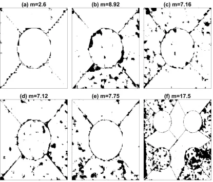
[image:10.595.90.505.138.618.2]Figure 7. (a–f) Results of the segmentation with U-Nets for the six texture arrangments. The misclassification (%) is shown in each case. Pixels that are correctly classified appear in white.
4. Discussion
The results provided by the U-Net algorithm provided interesting results in terms of the actual misclassification results against traditional algorithms, and the variability of the U-Net cases. The segmentation results provided by the U-Nets were better in four of the six images. In some cases, the results were very close to the second best option (a: 2.8/2.6, d: 7.3/7.1) and in two cases (e,f) traditional algorithms provided better results (e: 4.3/7.7, f: 17.0/17.5). The average for all the six composites was best for U-Nets, however, given the fact that the difference with the second best is relatively small (0.75), and that traditional algorithms provided better results in 1/3 cases shows that care should be taken when selecting algorithms. This is similar to the conclusion of Randen who stated that “No single approach did perform best or very close to the best for all images” [55].
In terms of texture, it can be highlighted that not all textures are the same, the five textures of image (a) are far easier to distinguish and correctly segment than those of image (b) and image (f). The U-Net was capable of segmenting these textures with accuracy comparable or better than traditional techniques. As mentioned previously, the fact that the textures have been histogram equalised removes the discrimination of the regions by their average intensities. More complex architectures, e.g., Siamese Networks [57] could provide better results, but it is important to use a standard benchmark such as that provided by Randen [55].
There are many other configuration parameters that could be varied; learning rate, batch size, variations of the training data, different number of layers, but for the purpose of this work, the results show first, the capability of deep learning architectures for segmentation of textured images and second, in some cases better results than traditional methodologies. However, the configuration of the network is not trivial and variations of some parameters can provide sub-optimal results. The experiments conducted in this work did not provide conclusive evidence for the selection of any of the parameters evaluated. Furthermore, training of the networks requires considerable resources. The training times for the images with 5 textures took around 5 hours and for the image with 16 textures around 96 hours on a Apple (Cuppertino, CA, USA) Mac Pro (Late 2013) with a 3.7 GHz Quad-Core and 32 GB Memory with Dual AMD FirePro D300 graphics processors.
Therefore, it can be concluded that U-Net convolutional neural networks can be used for texture segmentation and provide results that are comparable or better than traditional texture algorithms. Furthermore, these results encourage the application of deep learning to other areas. If we assume that different textures are characterised by patterns, i.e., repetitions of certain sequences or particular variation of intensities, then any data which is characterised by patterns could be analysed. For instance, phonemes in human speech have different patterns, which when combined form words. Thus one line of an image with different textures would have similar characteristics as the intensity variation of a phrase with different phonemes. Moreover, voice signals, which are one-dimensional can be converted into two-dimensional spectrograms [66] with time on one axis and frequency in another axis. In these cases, the spectrograms can be analysed for texture directly.
Author Contributions:Conceptualization: C.K., J.V., N.R.M. and C.C.R.-A.; Methodology C.K. and C.C.R.-A., writing, reviewing and editing, C.K., J.V., N.R.M. and C.C.R.-A.; funding acquisition J.V. and C.C.R.-A.
Funding:This work was funded by the Leverhulme Trust, Research Project Grant RPG-2017-054. C.K. is partially funded by the School of Mathematics, Computer Science and Engineering at City, University of London.
Conflicts of Interest:The authors declare no conflict of interest.
References
1. Bigun, J. Multidimensional Orientation Estimation with Applications to Texture Analysis and Optical Flow. IEEE Trans. Pattern Anal. Mach. Intell.1991,13, 775–790. [CrossRef]
2. Bovik, A.C.; Clark, M.; Geisler, W.S. Multichannel Texture Analysis Using Localized Spatial Filters. IEEE Trans. Pattern Anal. Mach. Intell.1990,12, 55 – 73. [CrossRef]
3. Cross, G.R.; Jain, A.K. Markov Random Field Texture Models.IEEE Trans. Pattern Anal. Mach. Intell.1983, 5, 25–39. [CrossRef] [PubMed]
4. Haralick, R.M. Statistical and Structural Approaches to Texture. Proc. IEEE1979,67, 786–804. [CrossRef] 5. Haralick, R.M.; Shanmugam, K.; Dinstein, I. Textural Features for Image Classification. IEEE Trans. Syst.
Man Cybern.1973,3, 610–621. [CrossRef]
6. Tamura, H.; Mori, S.; Yamawaki, T. Texture Features Corresponding to Visual Perception. IEEE Trans. Syst. Man Cybern.1978,8, 460–473. [CrossRef]
7. Tuceryan, M.; Jain, A.K. Texture Analysis. InHandbook of Pattern Recognition and Computer Vision, 2nd ed.; Chen, C.H., Pau, L.F., Wang, P.S.P., Eds.; World Scientific Publishing: Singapore, 1998; pp. 207–248. 8. Reyes-Aldasoro, C.C.; Bhalerao, A. The Bhattacharyya Space for Feature Selection and Its Application to
9. Bouman, C.; Liu, B. Multiple Resolution Segmentation of Textured Images. IEEE Trans. Pattern Anal. Mach. Intell.1991,13, 99–113. [CrossRef]
10. Jain, A.K.; Farrokhnia, F. Unsupervised Texture Segmentation using Gabor Filters. Pattern Recognit.1991, 24, 1167– 1186. [CrossRef]
11. Kadyrov, A.; Talepbour, A.; Petrou, M. Texture Classification with Thousand of Features. In Proceedings of the 13th British Machine Vision Conference (BMVC), Cardiff, UK, 2–5 September 2002; pp. 656–665. 12. Kervrann, C.; Heitz, F. A Markov Random Field Model-based Approach to Unsupervised Texture
Segmentation using Local and Global Spatial Statistics. IEEE Trans. Image Process. 1995, 4, 856–862. [CrossRef]
13. Unser, M. Texture Classification and Segmentation Using Wavelet Frames. IEEE Trans. Image Process.1995, 4, 1549–1560. [CrossRef] [PubMed]
14. Weszka, J.; Dyer, C.; Rosenfeld, A. A Comparative Study of Texture Measures for Terrain Classification. IEEE Trans. Syst. Man Cybern.1976,6, 269–285. [CrossRef]
15. Tai, C.; Baba-Kishi, K. Microtexture Studies of PST and PZT Ceramics and PZT Thin Film by Electron Backscatter Diffraction Patterns. Text. Microstruct.2002,35, 71–86. [CrossRef]
16. Carrillat, A.; Randen, T.; Snneland, L.; Elvebakk, G. Seismic Stratigraphic Mapping of Carbonate Mounds using 3D Texture Attributes. In Proceedings of the 64th EAGE Conference & Exhibition, Florence, Italy, 27–30 May 2002.
17. Randen, T.; Monsen, E.; Abrahamsen, A.; Hansen, J.O.; Schlaf, J.; Snneland, L. Three-dimensional Texture Attributes for Seismic Data Analysis. In Proceedings of the 70th SEG Annual Meeting, Calgary, AB, Canada, 6–11 August 2000.
18. Thybo, A.K.; Martens, M. Analysis of Sensory Assessors in Texture Profiling of Potatoes by Multivariate Modelling. Food Qual. Prefer.2000,11, 283–288. [CrossRef]
19. Létal, J.; Jirák, D.; Šuderlová, L.; Hájek, M. MRI ‘Texture’ Analysis of MR Images of Apples during Ripening and Storage. LWT Food Sci. Technol.2003,36, 719–727. [CrossRef]
20. Lizarraga-Morales, R.A.; Sanchez-Yanez, R.E.; Baeza-Serrato, R. Defect Detection on Patterned Fabrics using Texture Periodicity and the Coordinated Clusters Representation.Text. Res. J.2017,87, 1869–1882. [CrossRef] 21. Bianconi, F.; González, E.; Fernández, A.; Saetta, S.A. Automatic Classification of Granite Tiles through
Colour and Texture Features.Expert Syst. Appl.2012,39, 11212–11218. [CrossRef]
22. Kovalev, V.A.; Petrou, M.; Bondar, Y.S. Texture Anisotropy in 3D Images.IEEE Trans. Image Process.1999, 8, 346–360. [CrossRef]
23. Reyes-Aldasoro, C.C.; Bhalerao, A. Volumetric Texture Description and Discriminant Feature Selection for MRI. In Proceedings of the Information Processing in Medical Imaging, Ambleside, UK, 20–25 July 2003; Taylor, C., Noble, A., Eds.; pp. 282–293.
24. Lerski, R.; Straughan, K.; Schad, L.R.; Boyce, D.; Bluml, S.; Zuna, I. MR Image Texture Analysis—An Approach to tissue Characterization.Magn. Resonance Imaging1993,11, 873–887. [CrossRef]
25. Schad, L.R.; Bluml, S.; Zuna, I. MR Tissue Characterization of Intracranial Tumors by means of Texture Analysis.Magn. Resonance Imaging1993,11, 889–896. [CrossRef]
26. Reyes Aldasoro, C.C.; Bhalerao, A. Volumetric Texture Segmentation by Discriminant Feature Selection and Multiresolution Classification.IEEE Trans. Med. Imaging2007,26, 1–14. [CrossRef] [PubMed]
27. Zhan, Y.; Shen, D. Automated Segmentation of 3D US Prostate Images Using Statistical Texture-Based Matching Method. In Proceedings of the Medical Image Computing and Computer-Assisted Intervention (MICCAI), Montréal, QC, Canada, 15–18 November 2003; pp. 688–696.
28. Xie, J.; Jiang, Y.; tat Tsui, H. Segmentation of Kidney from Ultrasound Images based on Texture and Shape Priors. IEEE Trans. Med. Imaging2005,24, 45–57. [CrossRef] [PubMed]
29. Hoffman, E.A.; Reinhardt, J.M.; Sonka, M.; Simon, B.A.; Guo, J.; Saba, O.; Chon, D.; Samrah, S.; Shikata, H.; Tschirren, J.; et al. Characterization of the Interstitial Lung Diseases via Density-Based and Texture-Based Analysis of Computed Tomography Images of Lung Structure and Function.Acad. Radiol.2003,10, 1104–1118. [CrossRef]
31. Ganeshan, B.; Goh, V.; Mandeville, H.C.; Ng, Q.S.; Hoskin, P.J.; Miles, K.A. Non–Small Cell Lung Cancer: Histopathologic Correlates for Texture Parameters at CT.Radiology2013,266, 326–336. [CrossRef] [PubMed] 32. Sabino, D.M.U.; da Fontoura Costa, L.; Gil Rizzatti, E.; Antonio Zago, M. A Texture Approach to Leukocyte
Recognition. Real-Time Imaging2004,10, 205–216. [CrossRef]
33. Wang, X.; He, W.; Metaxas, D.; Mathew, R.; White, E. Cell Segmentation and Tracking using Texture-Adaptive Snakes. In Proceedings of the 2007 4th IEEE International Symposium on Biomedical Imaging: From Nano to Macro, Washington, DC, USA, 12–16 April 2007; pp. 101–104. [CrossRef]
34. Kather, J.N.; Weis, C.A.; Bianconi, F.; Melchers, S.M.; Schad, L.R.; Gaiser, T.; Marx, A.; Zollner, F. Multi-class Texture Analysis in Colorectal Cancer Histology.Sci. Rep.2016,6, 27988. [CrossRef] [PubMed]
35. Dunn, D.; Higgins, W.; Wakeley, J. Texture Segmentation using 2-D Gabor Elementary Functions.IEEE Trans. Pattern Anal. Mach. Intell.1994,16, 130–149. [CrossRef]
36. Bigun, J.; du Buf, J.M.H. N-Folded Symmetries by Complex Moments in Gabor Space and Their Application to Unsupervised Texture Segmentation. IEEE Trans. Pattern Anal. Mach. Intell.1994,16, 80–87. [CrossRef] 37. Bianconi, F.; Fernández, A. Evaluation of the Effects of Gabor Filter Parameters on Texture Classification.
Pattern Recognit.2007,40, 3325–3335. [CrossRef]
38. Rajpoot, N.M. Texture Classification Using Discriminant Wavelet Packet Subbands. In Proceedings of the 45th IEEE Midwest Symposium on Circuits and Systems (MWSCAS 2002), Tulsa, OK, USA, 4–7 August 2002. 39. Chang, T.; Kuo, C.C.J. Texture Analysis and Classification with Tree-Structured Wavelet Transform.
IEEE Trans. Image Process.1993,2, 429–441. [CrossRef]
40. Chellapa, R.; Jain, A.Markov Random Fields; Academic Press: Boston, MA, USA, 1993.
41. Krizhevsky, A.; Sutskever, I.; Hinton, G.E. ImageNet Classification with Deep Convolutional Neural Networks. In Proceedings of the 25th International Conference on Neural Information Processing Systems—Volume 1 (NIPS’12), Lake Tahoe, NV, USA, 3–6 December 2012; Curran Associates Inc.: New York, NY, USA, 2012; pp. 1097–1105.
42. Zeiler, M.D.; Fergus, R. Visualizing and Understanding Convolutional Networks. In Proceedings of the Computer Vision—ECCV 2014, Zurich, Switzerland, 6–12 September 2014; Fleet, D., Pajdla, T., Schiele, B., Tuytelaars, T., Eds.; Springer International Publishing: Berlin, Germany, 2014; pp. 818–833.
43. Simonyan, K.; Zisserman, A. Very Deep Convolutional Networks for Large-Scale Image Recognition.arXiv
2014, arXiv:1409.1556.
44. Russakovsky, O.; Deng, J.; Su, H.; Krause, J.; Satheesh, S.; Ma, S.; Huang, Z.; Karpathy, A.; Khosla, A.; Bernstein, M.; et al. ImageNet Large Scale Visual Recognition Challenge. Int. J. Comput. Vis. 2015, 115, 211–252. [CrossRef]
45. Andrearczyk, V.; Whelan, P.F., Chapter 4—Deep Learning in Texture Analysis and Its Application to Tissue Image Classification. InBiomedical Texture Analysis; Depeursinge, A., Al-Kadi, O.S., Mitchell, J.R., Eds.; Academic Press: Cambridge, MA, USA, 2017; pp. 95–129. [CrossRef]
46. Ronneberger, O.; Fischer, P.; Brox, T. U-Net: Convolutional Networks for Biomedical Image Segmentation. In Proceedings of the Medical Image Computing and Computer-Assisted Intervention—MICCAI 2015, Munich, Germany, 5–9 October 2015; Navab, N., Hornegger, J., Wells, W.M., Frangi, A.F., Eds.; Springer International Publishing: Berlin, Germany, 2015; Volume 9350, pp. 234–241.
47. Zhang, Z.; Liu, Q.; Wang, Y. Road Extraction by Deep Residual U-Net. IEEE Geosci. Remote Sens. Lett.2018, 15, 749–753. [CrossRef]
48. Jansson, A.; Humphrey, E.J.; Montecchio, N.; Bittner, R.M.; Kumar, A.; Weyde, T. Singing Voice Separation with Deep U-Net Convolutional Networks. In Proceedings of the 18th International Society for Music Information Retrieval Conference, Suzhou, China, 23–27 October 2017.
49. Dong, H.; Yang, G.; Liu, F.; Mo, Y.; Guo, Y. Automatic Brain Tumor Detection and Segmentation Using U-Net Based Fully Convolutional Networks. In Proceedings of the Annual Conference on Medical Image Understanding and Analysis, Edinburgh, UK, 11–13 July 2017; Valdés Hernández, M., González-Castro, V., Eds.; Springer International Publishing: Berlin, Germany, 2017; Volume 723, pp. 506–517.
50. Falk, T.; Mai, D.; Bensch, R.; Çiçek, Ö.; Abdulkadir, A.; Marrakchi, Y.; Böhm, A.; Deubner, J.; Jäckel, Z.; Seiwald, K.; et al. U-Net: Deep Learning for Cell Counting, Detection, and Morphometry.Nat. Methods2019, 16, 67. [CrossRef] [PubMed]
52. Ojala, T.; Pietikäinen, M.; Harwood, D. A Comparative Study of Texture Measures with Classification based on Feature Distributions. Pattern Recognit.1996,29, 51–59. [CrossRef]
53. Ojala, T.; Valkealahti, K.; Oja, E.; Pietikäinen, M. Texture Discrimination with Multidimensional Distributions of Signed Gray Level Differences. Pattern Recognit.2001,34, 727–739. [CrossRef]
54. Randen, T.; Husøy, J.H. Filtering for Texture Classification: A Comparative Study.IEEE Trans. Pattern Anal. Mach. Intell.1999,21, 291–310. [CrossRef]
55. Randen, T.; Husøy, J.H. Texture Segmentation using Filters with Optimized Energy Separation. IEEE Trans. Image Process.1999,8, 571–582. [CrossRef]
56. Brodatz, P.Textures: A Photographic Album for Artists and Designers; Dover: New York, NY, USA, 1996. 57. Yamada, R.; Ide, H.; Yudistira, N.; Kurita, T. Texture Segmentation using Siamese Network and Hierarchical
Region Merging. In Proceedings of the 2018 24th International Conference on Pattern Recognition (ICPR), Beijing, China, 20–24 August 2018; pp. 2735–2740. [CrossRef]
58. Petrou, M.; Garcia-Sevilla, P.Image Processing: Dealing with Texture; John Wiley & Sons: Hoboken, NJ, USA, 2006.
59. Reyes-Aldasoro, C.C.; Bhalerao, A.H. Volumetric Texture Analysis in Biomedical Imaging. InBiomedical Diagnostics and Clinical Technologies: Applying High-Performance Cluster and Grid Computing; Pereira, M., Freire, M., Eds.; IGI Global: Hershey, PA, USA, 2011; pp. 200–248.
60. Mirmehdi, M.; Xie, X.; Suri, J.Handbook of Texture Analysis; Imperial College Press: London, UK, 2009. 61. Vincent, L.; Soille, P. Watersheds in digital spaces: An efficient algorithm based on immersion simulations.
IEEE Trans. Pattern Anal. Mach. Intell.1991,13, 583–598. [CrossRef] 62. Gabor, D. Theory of Communication.J. IEE1946,93, 429–457. [CrossRef]
63. Knutsson, H.; Granlund, G.H. Texture Analysis Using Two-Dimensional Quadrature Filters. In Proceedings of the IEEE Computer Society Workshop on Computer Architecture for Pattern Analysis and Image Database Management—CAPAIDM, Pasadena, CA, USA, 12–14 October 1983; pp. 206–213.
64. Randen, T.; Husy, J.H. Multichannel filtering for image texture segmentation.Opt. Eng.1994,33, 2617–2625. [CrossRef]
65. Kingma, D.P.; Ba, J. Adam: A Method for Stochastic Optimization.arXiv2014, arXiv:1412.6980.
66. Verhoeven, J.; Miller, N.R.; Daems, L.; Reyes-Aldasoro, C.C. Visualisation and Analysis of Speech Production with Electropalatography.J. Imaging2019,5, 40. [CrossRef]
c