Vol 5, No 3 (2014)

Available online throug

ISSN 2229 – 5046

MICROPOLAR FLUID FLOW WITH VISCOELASTIC AND MASS TRANSFER EFFECTS

*I. J. Uwanta and **A. Hussaini

*Department of Mathematics, Usmanu Danfodiyo University Sokoto, Nigeria.

E-mail:

**Teachers Service Board Sokoto, Nigeria.

E-mail

(Received on: 06-02-14; Revised & Accepted on: 20-03-14)

ABSTRACT

T

he purpose of the present work is to study the influence of viscoelastic and mass transfer on unsteady MHD micropolar flow of incompressible and electrically conducting micropolar fluid past a semi-infinite vertical porous plate in the presence of a transverse magnetic field and periodic suction. Closed form solutions have been obtained for the mean velocity, mean angular velocity, mean temperature and mean concentration using perturbation technique and these are presented in graphical form. The effects of different physical parameters such as magnetic Hartmann number, thermal and solutal Grashof number, Prandtl number, Schmidt number, skin friction, heat transfer coefficient and Sherwood number are presented and discussed.

Keywords: Viscoelastic, Micropolar fluid,porous medium, thermal diffusion,variable suction.

INTRODUCTION

In numerous industrial transport processes, convective heat and mass transfer takes place simountaneously. Phenomena involving stretching sheets feature very widely in for example aerospace component production metal casting Dieter [1]. In such processes metals or alloys are heated until molten, poured into mould or die, and the liquid metal is subsequently stretched to achieve the desire product. When the super heated melt issues from the dies it loses heat and contract as it cools, a stage in metellurgical processing reffered to as liquid state contraction. With futher cooling and the loss of latent heat of fusion, the atoms of the metallic alloy loss energy and are bound tightly together in a regular structure. The mechanical properties of the final product depend to a great extent on the heat and mass transfer phenomena, the cooling rate, surface mass transfer rate etc. Much numerical researchhas been conducted in metal sheets flow including studies by Lait et. al. [2], Goldschmit et. al. [3] who examined viscoelastic metal flows. Goldschmit [4] who provides a finite element methodology for general metal flow forming.

Micropolar fluids are fluids with microstructure belonging to a class of complex fluids with nonsymmetrical stress tensor referred to as micromorphic fluids Aero et. al. [5]. Many numerical studies of micropolar heat and mass transfer have been communicated in the literature. Hassanian and Gorla [6] investigated the heat transfer to a micropolar fluid from a nonisothermal strectching sheet with suction and blowing. Flow over a porous strectching sheet with strong suction or injection was examined by Kelson and Farell [7]. Soudalgekar and Takher [8] have studied the effect of MHD forced and free convective flow past a semi-infinite plate. Raptis and Kafousias [9] studied the influence of a magnetic field upon the steady free convective flow through a porous medium bounded by an infinite vertical plate with a constant suction velocity and when the plate temperature is also constant.

Quite recently, a numerical study of steady combined heat and mass transfer by mixed convection flow past a continuously moving infinite vertical porous plate under the action of strong magnetic field with constant suction velocity, constant heat and mass fluxes have been investigated by Alam et. al. [10]. These type of problems play a spercial role in nature, in many separation processes as in isotope separation, in mixtures between gases, in many industrial applications as solidification of binary alloy as well as in astrophysical and geophysical engineering.

Corresponding author:

*I. J. Uwanta

*Department of Mathematics, Usmanu Danfodiyo University Sokoto, Nigeria.

FORMULATION OF THE PROBLEM

Consider the two-dimensional unsteady flow of a laminar, incompressible micropolar fluid past a semi-infinite vertical porous moving plate embedded in a porous medium and subjected to a transverse magnetic field in the presence of a pressure gradient. We assumed that there is no applied voltage which implies the absence of electric field. The transversely applied magnetic field and magnetic Reynolds number are very small and hence the induced magnetic field is neglegible Cowling [10]. It is also assumed that the size of the porous plate is significantly larger than a chracteristic microscopic length scale of the porous medium. Boussineq’s approximation for the equations of flow is governed as :

Continuity equation * *

0

v

y

∂

₌

∂

(1)

Linear momentum equation

(

)

(

)

* * * 2 * * *

2 * 0

* * * *2 * *

1

2

r f r

u

u

p

u

u

v

v

v

g

T

T

u

v

t

y

x

y

k

y

σ

ω

β

ν

β

ρ

ρ

∗ ∞

∂

₊

∂

_{= −}

∂

_{+ +}

∂

₊

₋

₋

₋

₊

∂

∂

∂

∂

∂

∂

(

)

3 1 *

0 * *2

u

K

g

C

C

t y

β

∂

−

+

− ∞

∂ ∂

(2)

Angular momentum equation * * 2 * *

* * *2

j

t

y

y

ω

ω

ω

ρ



∂

₊

ν

∗

∂



₌

γ

∂



_∂

_∂



_∂





(3)

Energy eqution 2

* * *2

T

T

T

v

t

y

α

y

∗

∂

₊

∂

₌

∂

∂

∂

∂

(4)

Concentrationequation

(

)

2

* * * *2

C

C

C

v

D

K

C

C

t

y

y

∗ ∗ ∗

∞

∂

₊

∂

₌

∂

₋

₋

∂

∂

∂

(5)

where

x y and t

∗

,

∗ ∗ are the dimensional distances along and perpendicular to the plate and dimensional time, respectively.

u and v

∗ ∗ are the components of dimensional velocities along

x and y

∗ ∗ direction,

ρ

is the fluid density,

σ

is the fluid electrical conductivity,

β

₀ is the magnetic induction,

j

∗the micro-inertia density of the component of the angular velocity vector normal to the

xy

−

plane

,

γ

the spine gradient viscosity,

v

is the fluid kinematic viscosity,

v

_ris the fluid kinematic rotational viscosity,

g

is the acceleration due to gravity,

β

_f

and

β

∗ are the coefficients of volume expansions for temperature and concentration,

k

∗ the permeability of the porous medium,

k

₀1 is the elastic parameter,

K

is the chemical reaction,

ω

∗ is the component of angular velocity,

T

is the temperature,

C

is the concentration ,

α

is the fluid thermal diffusivity.

The boundary conditions for the velocity, temperature and concentration fields are

(

)

(

)

(

)

(

)

0 2 2 0

,

1

,

,

,

0

1

,

,

,

0

n t n t

p

n t

n t

u

u v

v

e

T

T

T

T

e

u

C

C

C

C

e

at y

y

y

u

u

u

e

T

T C

C

where

u

_p∗ is the velocity of the moving plate,

T and C

_ω∗ _ω∗ are the temperature and the concentration respectively,

U

_∞∗

is the free stream velocity, and

U and n

₀ ∗ are constants. From equation (1), it is obvious that the suction velocity at the plate is either a constant or a function of time. Hence the suction velocity normal to the plate is assumedin the form

(

)

0

1

n t

v

∗

= −

V

+

ε

Ae

∗ ∗

(7) where

A

is a real positive constant,

ε

and

ε

A

is small values less than unity, and

V

₀ is the scale of suction velocity which is non-zero positive constant. The negative sign indicates that the suction is towards the plate.

Outside the boundary layer, equation (2) gives

* *

2 0 * * *

1

p

dU

U

U

x

dt

k

ν

_{σ β}

ρ

ρ

∗ ∗ ∗ ∞ ∞ ∞

∂

−

=

+

+

∂

(8)

To write the governing equations and the boundary conditions in dimensionless form, the following non-dimensional quantities are introduced

(

)

(

)

1

2

0 0

0 0 0 0 0 0 0

2 2 1 0 0 0 0

2 2 2

0 0 0

2 0

2 2 2

0 0 0 0 0

,

,

,

,

,

,

,

,

,

,

,

,

,

1

,

,

,

,

2

2

p p f

u

V y

U

t V

u

v

v

u

v

v

U

U

v

v

U

V

v

U

U

U V

V

k V

V j

T

T

C

C

T

T

n v

C

n

k

j

T

T

C

C

T

T

V

V

V

v

g T

T

v

g T

T

v

v

n

M

Gr

Gc

N

M

V

U V

U V

k

j

ω ω ω

ω ω

ω

θ

θ

β

β

σβ

α

ρ

µ

η

γ

∗ ∗ ∗ ∗ ∗ ∗ ∗ ∞ ∞ ∗ ∗ ∗ ∞ ∞ ∞ ∞ ∞ ∞ ∗ ∞ ∞ ∗

=

=

=

=

=

=

=

−

−

−

=

=

=

=

=

=

−

−

−

−

−

=

=

=

=

=

+

=

=

+

2 0

,

K

_r

K v

V

β

∗























=

_



(9)

In view of equations (7) – (9), equations (2) – (5) reduce to the following dimensional form.

(

1

)

(

1

)

22

(

)

2

3 2

nt

dU

u

u

u

u

Ae

Gr

N U

u

K

GcC

t

y

dt

y

y

t y

ω

ε

∞

β

θ

β

∞

∂

∂

∂

∂

∂

− +

=

+ +

+

+

− +

−

+

∂

∂

∂

∂

∂ ∂

(10)

(

)

2

2

1

1

Ae

nt

t

y

y

ω

_ε

ω

ω

η

∂

_{− +}

∂

₌

∂

∂

∂

∂

(11)

(

)

2

2

1

1

Pr

nt

Ae

t

y

y

θ

_ε

θ

θ

∂

∂

∂

− +

=

∂

∂

∂

(12)

(

)

2

2

1

1

nt

C

C

C

Ae

KC

t

ε

y

Sc y

∂

_{− +}

∂

₌

∂

₋

∂

∂

∂

(13)

where

_N

_M

1

_{and Gr Gc Pr K and Sc}

_,

_,

_,

_,

k

=

+

are the thermal Grashof number, solutal Grashof number, Prandtl number, chemical reaction parameter and Schmidt number respectively.

The dimensionless form of the boundary conditions (6) becomes

(

)

2

2

,

1

,

1

,

1

,

0

,

0,

0,

0,

nt nt nt

p

u

u

u v

Ae

e

C

e

at y

y

y

u

u

C

as y

ω

ε

θ

ε

ε

θ

ω

∞



∂

∂

=

= − +

= +

= +

= −

_{= }

∂

∂





→

→

→

→

→ ∞

_

(14)

( )

( )

( )

( )

( )

( )

( )

( )

( )

( )

( )

( )

2 0 1 2 0 1 2 0 1 2 0 1

0

0

0

0

nt nt nt nt

u

u

y

e u

y

y

e

y

y

e

y

C

C

y

e C

y

ε

ε

ω ω

ε ω

ε

θ θ

ε θ

ε

ε

ε



=

+

+





=

+

+

_



=

+

+

_



=

+

+

_

(15)

Substituting (15) in equations (10)–(13) and equating the harmonic and non–harmonic terms, and neglecting the higher order terms of

0

( )

ε

2 , we obtain

(

1

+

β

)

u

0

′′

+ −

u

0

′

Nu

0

= − −

N

Gr

θ

0

−

GcC

0

−

2

βω

0

′

(16)

(

)

(

)

1 1 1 0 1 1

2

1

Eu

′′

+ −

u

′

N

+

n u

= −

N

+ −

n

Au

′

−

Gr

θ

−

GcC

−

βω

′

(17)

0 0

0

ω ηω

′′

+

′

=

(18)

1 1

n

1

A

0

ω ηω

′′

+

′

−

ηω

= −

ηω

′

(19)

0

Pr

0

0

θ

′′

+

θ

′

=

(20)

1

Pr

1

n

Pr

1

A

Pr

0

θ

′′

+

θ

′

−

θ

= −

θ

′

(21)

0 0 r 0

0

C

′′

+

ScC

′

−

k ScC

=

(22)

(

)

1 1 r 1 0

C

′′

+

ScC

′

− +

n k ScC

= −

AScC

′

(23) where primes denote ordinary differentiation with respect to

y

.

The corresponding boundary conditions can be written as

0 1 0 1 1 0 1 0 1

0 1 0 1 0 1 0 1

,

0,

,

,

1,

1,

1,

1

0

1,

1,

0,

0,

0,

0,

0,

0

p

u

u u

u

u

C

C

at y

u

u

C

C

as y

ω

ω

θ

θ

ω

ω

θ

θ

′′

′′

=

=

= −

= −

=

=

=

=

=





→

→

→

→

→

→

→

→

_{→ ∞}

(24)

Solving equations (16)–(23) under the boundary conditions (24) we obtain the linear velocity, angular velocity, temperature and concentration distribution in the boundary layer as

( )

2 1

4 6 7 8

,

1

m y Pry m y y

u y t

= +

B e

−

+

B e

−

+

B e

−

+

B e

−η

7 5 6

4 2 1

15 18 21 23

25 26 27 28

1

m y Pry m y m y

nt

m y m y m y y

B e

B e

B e

B e

e

B e

B e

B e

B e

η

ε





+

−

+

₋ −

+

₋−

+

₋−

+

₋





+

_

_

+

+

+









(25)

( )

(

4

)

1 9 10

,

y nt m y y

y t

B e

η

e

B e

B e

η

ω

₌

−

₊

ε

−

₊

−

(26)

( )

1

(

5 1

)

2 11 12

,

m y nt m y m y

y t

B e

e

B e

B e

θ

₌

−

₊

ε

−

₊

−

(27)

( )

2

(

6 2

)

3 13 14

,

m y nt m y m y

C y t

=

B e

−

+

ε

e

B e

−

+

B e

− (28) where

(

2

)

1

1

4

,

2

r

m

=

Sc

+

S c

+

ScK

₁

1

(

2

4

)

,

2

r

m

=

Sc

+

S c

+

ScK

₃

1

1

4

,

2

n

m

η

η





=

_

_

+

+

_

_





4

4

1

1

,

2

Pr

n

m

Pr





=

_

_

+

+

_

_





(

)

5

1

1 4

,

2

n

k

Sc

m

Sc



₊







=

+

+









6

(

(

)

)

1

1

1 4

,

2

m

N

n E

E

=

+

+

+

1 10

,

A B

B

n

η

−

=

A

₈

=

u

_p

− +

(

1

A

₁₀

+

A

₁₁

+

A

₁₂

)

,

(

)

11 2 1 1

,

1

Gm

A

m

m

N

β

−

=

+

−

−

(

)

2

12 2

2

1

A

A

N

βη

β η η

=

+

− −

, 2 15

,

AA

A

n

η

−

=

A

₁₄

= −

(

u

₁

+

A

₁₅

)

,

18

,

APr

A

n

−

=

A

₁₇

= −

1

A

₁₈

,

(

)

1 21 2 1 1

,

m ASc

A

m

m Sc

n

k Sc

=

−

− +

A

20

= −

1

A

21

,

_,

(

)

2 8 25 2 2 2

,

m A

A

Em

m

N

n

=

−

−

+

(

)

10 26 2

Pr

,

A

A

EP r

Pr

N

n

=

(

)

1 11 27 2 1 1

,

m A

A

Em

m

N

n

=

−

−

+

28 2

(

12

)

,

A

A

E

N

n

η

η η

−

=

− −

+

(

)

17 29 2 4 4

,

GA

A

Em

m

N

n

−

=

−

−

+

(

)

3 14 33 2 3 3

2

,

m A

A

Em

m

N

n

β

=

−

−

+

(

)

18

30 2

,

P r

GA

A

E

Pr

N

n

−

=

−

−

+

31 2

(

)

5 5

,

Gm

A

Em

m

N

n

−

=

−

−

+

(

15

)

34 2

2

,

A

A

E

N

n

βη

η η

=

− −

+

(

)

21 32 2 1 1

,

GmA

A

Em

m

N

n

−

=

−

−

+

(

)

15

1

17 18 19 20 21 22 23 24 25 26

B

= − +

B

+

B

+

B

+

B

+

B

+

B

+

B

+

B

+

B

+

B

,

It is essential to calculate the physical quantities of primary interest, which are the Skin – friction, Nusselt number and the Sherwood number. Given the velocity field in the boundary layer, we can calculate the Skin – friction given by

[

{

2 4

Pr

6 1 7 8 7 15

Pr

18 5 21 6 23

nt f

C

= −

m B

+

B

+

m B

+

η

B

+

ε

e

m B

+

B

+

m B

+

m B

+

m B

4 25

+

m B

2 27

+

m B

1 28

+

η

B

29

]

}

(29) Knowing the temperature field,heat transfer coefficient can be obtained in terms of the Nusselt number, given by

0 1 0 0 nt u y y

N

e

y

y

y

θ

θ

θ

_ε

= =



∂





∂

∂



=

_

_

=

_

+

_

∂

∂

∂









(

4 17

Pr

18

)

nt u

N

= −



_

Pr

+

ε

e

m A

+

A



_

(30) Knowing the concentration field, the rate of mass transfer coefficient can be obtalned in terms of the Sherwood, is given by 0 1 0 0 nt h y y

C

C

C

S

e

y

₌

y

ε

y

₌



∂





∂

∂



=

_

_

=

_

+

_

∂

∂

∂









(

)

1 5 20 1 21

nt h

S

= −



_

m

+

ε

e

m A

+

m A



_

(31)

RESULTS AND DISCUSSION

Graphical representation of results is very useful to discuss the physical features presented by the solutions. In order to get a physical insight into the problem, factors such as streamline velocity, angular velocity, temperature, concentration, skin friction, nusselt number and sherwood number have been discussed by assigning numerical values to various parameters obtained in the mathematical formulation of the problem and the results are graphically presented in Figures 1- 17. Unless otherwise stated, throughout the computations we have chosen

K

₀

=

0.3,

K

_r

=

0.3,

M

=

1,

2.0,

1.0,

0.71,

0.2,

0.2,

_p

0.5,

1.0,

Gc

=

Gr

=

Pr

=

Sc

=

β

=

U

=

n

=

t

=

1.0,

ε

=

0.02.

The velocity distribution is shown in Figures 1- 11 for different values of the parameters

M Gr Gc Sc Pr K K t

,

,

,

,

,

₀

,

_r

, ,

,

U

_p

β

and

ε

respectively. The increment of Hartmann magnetic number M decreases the velocity of the fluid. As usual the Grashof number for local heat and mass transfer boost the fluid velocity, hence is found that the effect of increasing

Gr

and

Gc

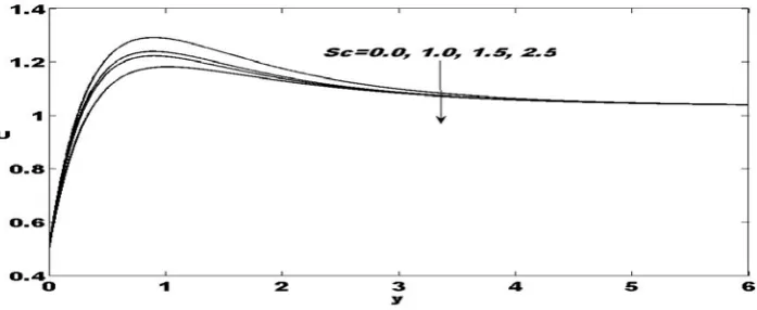
increase the velocity field as expected Figures 1- 3. Figures 4 and 5 reveals the mean velocity profiles due to variations in

Sc and Pr

. It is noticed that whenever Schmidt number increases the mean velocity decreases. It is further observed that increases in Prandtl number causes the decrease in mean velocity. Figures 6 – 7 are graphed to see the influence of viscoelastic parameter

K

₀and chemical reaction

K

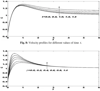
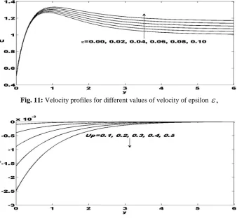
_r respectively. It is observed that the increment of viscoelastic parameter and chemical reaction parameter decrease the velocity of the fluid. In Figures 8,9,10 and 11 increasing the time

t

, viscosity ratio

β

,

velocity of the moving plate

U

_pand material parameter epsilon

ε

,

increases the velocity.

The variation of temperature field along the

y

- axis is shown in Figure 15 indicates the effects of Prandtl number

Pr

.

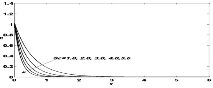
The Prandtl number defines the ratio of momentum diffusivity to thermal diffusivity. It is observed that increase in the Prandtl number results a decrease of the thermal boundary layer thickness and therefore lower average temperature within the flow because increasing values of Prandtl number equivalent to increase the thermal conductivities and therefore heat is able to diffuse away from the heated plate more rapidly.

The variation of the mass concentration along

y axis

−

is dipict in Figures 16 and 17 respectivily for different varying values of chemical reaction parameter

K

_r and Schmidt number

Sc

. It is observed that for the increase of chemical reaction and Schmidt number the concentration decreases.

It is observed from table (1) that as effects of

M Gr and Gc

,

increases , the skin – friction coefficients increases whereas the Nusselt and the Sherwood numbers remain unchanged. As effect of

Sc

increases the skin – friction coefficient decreases and the Sherwood number increases while the Nusselt number remain unchanged. It is noticed that as the

Pr

increases both the Skin – friction coefficient and the Nusselt numbers decreases and the Sherwood number remain unchanged. Increasing the effects of

K

₀ results in a decreasing of the Skin – friction coefficient and both the Nusselt and the Sherwood numbers are unchanged. It is also observed from the table that as the effects of

K

_r

increases the the skin - friction coefficient and the Sherwood number decreases whereas the Nusselt number is unchanged.

CONCLUSION

In this paper we have investigated the influence of viscoelastic and mass transfer on unsteady MHD micropolar fluid flow of incompressible and electrically conducting micropolar fluid past a semi-infinite vertical porous plate in the presence of transverse magnetic field by using perturbation method. The effects of various parameters entering into the problem have been discussed in detail. From the investigation we notice the following observations.

When the Hartmann magnetic parameter is high and the dimensionless velocity gradient is lower, the magnetic effect will decrease the momentum force and the flow will move slowly with the whole flow field and the magnetic effect is not good for a larger magnetic parameter. It is observed that increasing the value of Prandtl number equivalent to increase the thermal conductivities and therefore heat is able to diffuseaway from the heated plate more rapidly. Hence in the case of increasing Prandtl number, the boundary layer is thinner and the heat transfer is reduced.

When the thermal and solutal Grashof numbers were increased, the thermal and concentration buoyancy effects were enhenced and thus, the fluid velocity increased.

Fig. 2: Velocity profiles for different values of thermal Grashof number

Gr

,

Fig. 3: Velocity profiles for different values of solutal Grashof number

Gc

,

Fig. 4: Velocity profiles for different values of Schmidt number

Sc

,

Fig. 6: Velocity profiles for different values of viscoelastic parameter

K

₀

,

Fig. 7: Velocity profiles for different values ofchemical reaction parameter

K

_r

,

Fig. 8: Velocity profiles for different values of time

t

.

Fig. 10: Velocity profiles for different values of velocity of moving plate

U

_p

,

Fig. 11: Velocity profiles for different values of velocity of epsilon

ε

,

Fig. 12: Angular velocity profiles for different values of moving plate velocity

U

_p

,

Fig. 14: Angular velocity profiles for different values of time

t

,

Fig. 15: Temperature profiles for different values of Prandtl number

Pr

,

Fig. 16: Concentration profiles for different values of chemical reaction

K

_r,

Fig. 17: Concentration profiles fordifferent values of Schmidt

Sc

,

M Gr Gc Sc Pr K0 Kr K Cf Nu Sh 1.00 1.00 2.00 0.20 0.71 0.30 0.30 0.50 2.5138 -0.7867 -1.3122 2.00 1.00 2.00 0.20 0.71 0.30 0.30 0.50 2.5461

1.00 2.00 2.00 0.20 0.71 0.30 0.30 0.50 2.9374 1.00 1.00 3.00 0.20 0.71 0.30 0.30 0.50 2.8628

1.00 1.00 2.00 0.30 0.71 0.30 0.30 0.50 2.5006 -1.3707 1.00 1.00 2.00 0.20 0.81 0.30 0.30 0.50 2.4952 -0.8961

1.00 1.00 2.00 0.20 0.71 0.40 0.30 0.50 2.4985

1.00 1.00 2.00 0.20 0.71 0.30 0.40 0.50 2.5036 -1.3574 1.00 1.00 2.00 0.20 0.71 0.30 0.30 0.60 2.4911

REFERENCES

[1] G.E. Dieter (1986), Mechanical Metallurgy, New York, McGraw-Hill.

[2] Lait, J.E. and J.K. Brimacomibe, J.K. and Weinberg, F. (1974), Mathematical modeling of heat flow in the continous casting of steel, Ironmaking and Steelmaking Quarterly J, 2, Pp. 90-97.

[3] Goldschmit M.B., Gonzalez, J.C. and Dvorkin E.N. (1993), On a finite element model for analyzing the liquid metal development during continous casting of round bars, Ironmaking and Steelmaking Quarterly J, 20, Pp. 379-385. [4] M.B. Goldschmit M.B. (1997), Computational fluid mechanics application in continous casting,int. Proc. 80th Steelmaking Conf. Chicago, EEUU.

[5] Aero, E.L., Bulygin, A.N. and Kuvshinski, E.V. (1965), Asymmetric hydromechanics, J. Appl. Math. Mech., 29, Pp.333-346.

[6] Hassanien I.A. and Gorla R.S.R. (1990), Mixed convection boundary layer flow of a micropolar fluid near a stagnation point on a horizontal cylinder, Acta Mech, 84, Pp.191-199.

[7] Kelson N.A. and Farell T.W. (2001), Micropolar flow over a porous strectching sheet with strong suction or injection, Int. Comm. Heat Mass Transfer, 28, Pp. 479-488, 2001.

[8] Soudalgekar, V.M. andTakher, H.S. (1997), MHD forced and free convective flow past a semi-infinite plate, AIAA J, 15, Pp. 457-458.

[9] Raptis, A.A. and Kafousias, N. (1982), Heat transfer in flow through a porous medium bounded by an infinite vertical plate under the action of a magnetic field. Int. J. Energy Research, 6, Pp. 241-245.

[10] Alam et al. (2008), Micropolar fluid behaviour on MHD heat transfer flow through a porous medium with induced magnetic field by finite difference method, Thomas Int. J. of Science and Technology, 4, Pp.13.