A joint regression modeling framework for analyzing bivariate binary data in R

City, University of London Institutional Repository

Citation

:

Marra, G. and Radice, R. ORCID: 0000-0002-6316-3961 (2017). A joint

regression modeling framework for analyzing bivariate binary data in R. Dependence

Modeling, 5(1), pp. 268-294. doi: 10.1515/demo-2017-0016

This is the published version of the paper.

This version of the publication may differ from the final published

version.

Permanent repository link: http://openaccess.city.ac.uk/21060/

Link to published version

:

http://dx.doi.org/10.1515/demo-2017-0016

Copyright and reuse:

City Research Online aims to make research

outputs of City, University of London available to a wider audience.

Copyright and Moral Rights remain with the author(s) and/or copyright

holders. URLs from City Research Online may be freely distributed and

linked to.

City Research Online:

http://openaccess.city.ac.uk/

publications@city.ac.uk

Research Article

Open Access

Giampiero Marra* and Rosalba Radice

A joint regression modeling framework for

analyzing bivariate binary data in

R

https://doi.org/10.1515/demo-2017-0016

Received September 22, 2017; accepted October 18, 2017

Abstract:_{We discuss some of the features of the}Radd-on packageGJRMwhich implements a flexible joint

modeling framework for fitting a number of multivariate response regression models under various sampling schemes. In particular, we focus on the case in which the user wishes to fit bivariate binary regression models in the presence of several forms of selection bias. The framework allows for Gaussian and non-Gaussian de-pendencies through the use of copulae, and for the association and mean parameters to depend on flexible functions of covariates. We describe some of the methodological details underpinning the bivariate binary models implemented in the package and illustrate them by fitting interpretable models of different complex-ity on three data-sets.

Keywords:binary data, copula, confounding, joint model, penalized smoother, selection bias,R,

simultane-ous parameter estimation

MSC:62H99, 62J02

1 Introduction

TheR[43] packageGJRM[Generalised Joint Regression Modelling, 34] implements a flexible joint modeling framework for fitting a number of multivariate response regression models under various sampling schemes. The package currently contains two main fitting functions:gjrm()which fits bivariate regression models with binary, discrete, continuous and survival margins in the presence of associated responses, endogeneity and non-random sample selection, and trivariate binary models with and without double sample selection; gamlss()which fits several flexible univariate regression models (this was initially designed to provide start-ing values for many of the joint models in the package but it was subsequently made available in the form of a proper function). This paper focuses on the case in which the user wishes to fit bivariate binary models in the presence of (i) endogeneity, (ii) non-random sample selection or (iii) partial observability. We illustrate the capabilities of such tool by fitting interpretable models of different complexity on real data. The literature on models tackling selection bias is vast and many variants have been proposed. Since our focus is on the case of binary data, all of the non-binary cases (such as those mentioned above) are not discussed here since these would deserve separate and lengthy expositions. The models considered in this article have wide ap-plicability. Some examples are given by [9], [17], Jeliazkov and Yang [26, Chapter 13], [27], [29], [40] and [48], to name but a few. The next sections describe the three aforementioned issues and available approaches to tackle them.

*Corresponding Author: Giampiero Marra:Department of Statistical Science, University College London, Gower Street,

Lon-don WC1E 6BT, UK, E-mail: giampiero.marra@ucl.ac.uk

Rosalba Radice:Department of Economics, Mathematics and Statistics, Birkbeck, University of London, Malet Street, London

1.1 Endogeneity

Quantifying the effect of a non-randomly assigned treatment on an outcome may be a challenging task in the presence of unobserved confounders (i.e., unknown or not readily quantifiable variables associated with both treatment and outcome). In this situation, the treatment is often termed endogenous and the bias re-sulting from neglecting unobserved confounding is typically referred to as endogenous selection bias. For the case of binary treatment and outcome, [21] introduced the bivariate probit model to address this issue (see also [18] and [30] for a gentle introduction). Alternative approaches are discussed in the excellent review by [11] which empirically shows that all methods considered (including the bivariate probit) produce very similar results. [10] and [31] extended Heckman’s model by introducing Bayesian and likelihood penalized spline methods to model flexibly covariate-response relationships. To account for non-Gaussian dependence between treatment and outcome, [55] discussed the use of copulae. [44] proposed a more general approach that deals simultaneously with unobserved confounding, non-linear covariate effects and non-Gaussian de-pendence between treatment and outcome, and incorporated these developments inGJRM. Specifically, the conventional bivariate probit model (which does not model flexibly covariate effects in a data-driven man-ner and does not account for non-Gaussian dependencies) can be fitted inSAS[25] using the built-inproc qlim[24] and inStata[52] using the built-in functionsbiprobit[51],mvprobit[8] andssm[37]. InR,VGAM [60] may be used to estimate a bivariate binary model with endogenous treatment and non-linear covariate effects but it relies on the assumption of Gaussian errors.mvProbit[23] may also be employed but it is under development.

1.2 Non-random sample selection

Survey data (but not only) are often affected by systematic non-participation. This can occur through a variety of mechanisms, including directly declining to participate in the study. If individuals select themselves into (or out of) the sample based on a combination of observed and unobserved characteristics then models that ignore such a mechanism will most likely yield estimates which are not representative of the population of interest. The bias arising from neglecting this systematic non-participation is typically known as non-random sample selection bias. Selection and pattern-mixture models can deal with this issue, even when selection is based on unobserved characteristics of respondents; Fitzmaurice et al. [15, Chapter 18] provide a discussion of the features and variants of both approaches. Here the focus is on the sample selection model approach which was introduced by [19], [28] and [20], and discussed more thoroughly in [22]. When the outcome is binary, the conventional selection model is a bivariate probit [13, 54]. [35] proposed, and incorporated inGJRM, a selection model which allows for Gaussian and non-Gaussian dependencies, arbitrary parametric link functions, and for the association and mean parameters to depend on several types of smooth functions of covariates; this work extended the scope of the approaches introduced by [32] and [36]. More restrictive bivariate selection models, which rely on normality and on linear or pre-specified non-linear covariate-response relationships, can be fitted inSASusing theproc qlim, inStatausing the built-in commandsheckprob[51],mvprobitand ssm, and inRusingsampleSelection[53].

1.3 Partial observability

applications of this model. The bivariate binary model with partial observability can be fitted inStatausing biprobit. In this work we have extended the model to include flexible covariate effects, and incorporated it inGJRM.

The paper is organized as follows. Section 2 introduces a general modeling framework for analyzing bivariate binary data. Section 3 then discusses in more detail the binary models considered in this paper. Section 4 provides an overview ofgjrm()inGJRM, whereas Section 5 is devoted to three data examples that illustrate the use of the software. Section 6 concludes the paper.

2 Methodology

Let us assume that there are two binary random variables (Y_i1,Y_i2), fori= 1,. . .,n, wherenrepresents the

sample size. The probability of event (Yi1= 1,Yi2= 1) can be defined as

p_11i=P(Y_i1= 1,Y_i2= 1) =C(P(Y_i1= 1),P(Y_i2= 1);θ_i),

whereP(Yij= 1) = 1−Fj(−ηji) forj= 1, 2,Fj(·) is the cumulative distribution function (cdf) of a standardized

univariate distribution (in this case Gaussian, logistic or Gumbel),η_ji ∈ Ris an additive predictor (refer

to (2) below),C is a two-place copula function [49, 50] andθi is an association parameter measuring the

dependence between the two random variables. The notation adopted for defining P(Y_ij = 1) is perhaps

unusual. However, here we have exploited the link between the binary regression model andY_ij* = ηji +

ϵ_i, whereY_ij* is a continuous latent variable,ϵ_iis an error term andY_ij can be viewed as an indicator for Y*_ij > 0. Therefore,P(Yij = 1) =P(Yij* > 0) = 1 −Fj(−ηji). The marginal cdfs are conditioned on covariates

throughη_1iandη_2i, but for notational convenience we have suppressed this when expressing them. Since

the strength and direction of the association between the two marginals may, for instance, vary across groups of observations, the dependence parameter is specified as a function of an additive predictor. That is,θ_i = m(ηci), wheremis a one-to-one transformation which ensures thatθilies in its range. This approach follows

the same rationale of [45], who introduced generalized additive models for location, scale and shape, where all the parameters characterizing a chosen distribution are related to predictors via suitable link functions. The copulae implemented inGJRM, corresponding ranges ofθand list of transformationsm(·) are reported

in Table 1 of [33]. Rotations by 90◦_{, 180}◦_{and 270}◦_{are also implemented; for example, rotating the Clayton,} Gumbel and Joe by 90◦_{and 270}◦_{allows these copulae to model negative dependence. Parameterθis often} not easy to interpret, in which case the well known Kendall’sτ∈[−1, 1] can be employed. For full details on copulae see, for instance, [38].

The log-likelihood function of the sample can be expressed as

`=

n

X

i=1







1

X

a,b=0

1abilog(pabi)







, (1)

where1abiis an indicator function equal to one when (yi1=a,yi2=b) is true,a,b∈ {0, 1}, andyi1andyi2

are realizations ofYi1andYi2, respectively.

2.1 Additive predictor specification

Let us consider a generic additive predictorη_νiand an overall covariate vectorz_νi. Here, subscriptνcan take

values 1, 2 (which refer to the first and second margins) andc (which refer to the copula parameter). The

predictor can be defined as

η_νi=βν0+

Kν

X

kν=1

whereβν0 ∈Ris an overall intercept,zνkνidenotes thek

th

ν sub-vector of the complete vectorzνiand theKν

functionss_νkν(z_νkνi) represent generic effects which are chosen according to the type of covariate(s)

consid-ered. Eachsνkν(zνkνi) can be approximated as a linear combination ofQνkν basis functionsbνkνqνkν(zνkνi) and

regression coefficientsβ_νkνq

νkν ∈R, i.e.

s_νkν(z_νkνi) =

Q_νkν

X

q_νkν=1 β_νkνq

νkνbνkνq_νkν(zνkνi). (3)

Equation (3) implies that the vector of evaluations

s_νkν(z_νkν1),. . .,s_νkν(z_νkνn) Tcan be written asZ_νkνβ_νk

ν

withβ_νkν = (βνkν1,. . .,βνkνQνkν)

T_{and design matrixZ}

νkν[i,qνkν] =bνkνqνkν(zνkνi). This allows the predictor in

equation (2) to be written as

η_ν=βν01n+Zν1βν1+. . .+ZνKνβνKν, (4)

where1nis ann-dimensional vector made up of ones. Equation (4) can also be written in a more compact

way asη_ν=Zνβ_ν, whereZν= (1n,Zν1,. . .,ZνKν) andβν= (βν0,βTν1,. . .,β

T

νKν)

T_{. Eachβ}

νkhas an associated

quadratic penaltyλ_νkνβT_νkνD_νkνβ_νkν, used in fitting, whose role is to enforce specific properties on thekthν

func-tion, such as smoothness. For the case of a smooth function of a continuous regressorz_νkν,D_νkν may be

cal-culated asR

d_νkν(z_νkν)d_νkν(z_νkν)Tdz_νkν, where theqth_νk

νelement ofdνkν(zνkν) is given by∂2bνkνq_νkν(zνkν)/∂z2νkν

and integration is over the range ofz_νkν. See, for instance, [33] for other examples. The smoothing

param-eterλ_νkν ∈ [0, ∞) controls the trade-off between fit and smoothness, and plays a crucial role in determin-ing the shape of ˆs_νkν(z_νkνi). Let us consider again the case of a smooth effect of a continuous variable. A

value ofλ_νkν = 0 (i.e., no penalization is imposed during fitting) will result in an un-penalized regression

spline estimate which will most likely over-fit the data, whileλ_νkν → ∞ (i.e., the penalty has a large in-fluence on the smooth function) will lead to a straight line estimate. The overall penalty can be defined as βT_νDνβν, whereDν = diag(0,λν1Dν1,. . .,λνKνDνKν). The smoothing parameters can be collected in vector

λν= (λν1,. . .,λνKν)

T_{. Finally, smooth functions are typically subject to centering (identifiability) constraints}

(see [58] for more details).

The above formulation allows one to employ a rich variety of covariate effects. Specifically,GJRMcan accommodate all terms available inmgcv[59], which include smooth functions of continuous covariates, smooth interactions between continuous and/or discrete variables, random effect smoothers and spatial smoothers for data sampled over a large portion of the globe or for geographic areas with complicated bound-aries. These are incorporated in our modeling framework by specifying the appropriateZ_νkν andD_νkν.

Oth-erwise, the construction of the additive predictors and overall smoothing penalty remains essentially un-changed.

2.2 Parameter estimation

Our model specification allows for a high degree of flexibility in modeling covariate effects. If an unpenalised approach is employed to estimate the model’s paramters then over-fitting is the likely consequence [e.g., 46]. To prevent this, we maximize

`p(δ) =`(δ) − 12δTSδ, (5)

where`pis the penalized model’s log-likelihood,δT= (βT₁,βT₂,βTc) andS= diag(D1,D2,Dc). The smoothing

parameter vectors are collected in the overall vectorλ= (λT₁,λT₂,λTc)T. In practice, estimation ofδandλis

2.3 Further considerations

At convergence, point-wise ‘confidence’ intervals for linear and non-linear functions of the model’s coeffi-cients can be obtained using the Bayesian large sample approximation

δ∼· N(ˆδ,V_δ), (6)

where ˆδis a parameter vector estimate,Vδ = −Hp(ˆδ)−1andHp is the penalized model’s Hessian.

Inter-vals derived using (6) have good frequentist properties since they account for both sampling variability and smoothing bias; see [35] and references therein for details. Intervals for non-linear functions of the model’s coefficients (e.g.,τ, joint and conditional predicted probabilities) can be conveniently obtained by simulation

from the posterior distribution ofδusing the following steps:

1. Drawnsimrandom vectors fromN(ˆδ,Vδ).

2. Calculaten_simsimulated realizations of the quantity of interest. For instance, for a Gaussian copulaτ_i= 2

πarcsin

tanh

ηci(Zci;βc) in which caseτsimi = (τsimi 1,τ sim2

i ,. . .,τ sim_nsim

i )T∀i= 1,. . .,nis obtained

usingβsimj

c ∀j= 1,. . .,nsim.

3. For eachτsim_i , calculate the lower,ς/2, and upper, 1 −ς/2, quantiles.

A small value fornsim, say 100, typically gives accurate results, whereasςis usually set to 0.05.

Model building in our framework involves the choice of copula function, of pair of link functions and se-lection of relevant covariates in the model’s additive predictors. To this end, we recommend using the Akaike information criterion (AIC) and/or the Bayesian information criterion (BIC), and hypothesis testing. The AIC and BIC are given by −2`(ˆδ)+2edfand −2`(ˆδ)+log(n)edf, where the log-likelihood is evaluated at the

penal-ized parameter estimates andedfrepresents the effective degrees of freedom (see [35] for the exact definition).

Approximate p-values for testing smooth components for equality to zero are obtained using the results by Wood [56] and Wood [57].

3 The models

In the following sections, we describe in some detail the three models that can deal with the issues of (i) endogeneity, (ii) non-random sample selection and (iii) partial observability, discuss their additive predictor specifications and log-likelihood functions. We also report some typical measures of interest. For more details on the models dealing with (i) and (ii), the reader is to referred to [44] and [35].

3.1 Bivariate binary model with endogenous treatment

A bivariate binary model with endogenous treatment is mainly employed when one is interested in estimat-ing the effect of a binary treatment on a binary outcome in the presence of unobserved confoundestimat-ing. In eco-nomics, this problem is commonly framed in terms of a regression model from which important covariates have been omitted and hence become a part of the model’s error term. In this context, the treatment is termed exogenous if it is not associated with the error term after conditioning on the observed confounders, and endogenous otherwise. The bivariate model controls for unobserved confounding by using a two-equation structural latent variable framework where one equation essentially describes a binary outcome (sayY_i2) as a

function of a binary treatment (Yi1) whereas the other equation determines whether the treatment is received.

the additive predictors for this model can be expressed as

η₁=β₁₀1n+Z₁₁β₁₁+. . .+Z₁K1β1K1 =Z1β1,

η₂=β₂₀1n+β₂₁y₁ +. . .+Z₂K2β2K2 =Z2β2,

η_c=βc01n+Zc1βc1+. . .+ZcKcβcKc =Zcβc,

whereas log-likelihood function (1) becomes

`=

n

X

i=1

111ilog(p11i) +110ilog(p10i) +101ilog(p01i) +100ilog(p00i) ,

wherep₁₀i=

1 −F₁(−η₁i) −p11i,p01i=

1 −F₂(η₂i) −p11iandp00i= 1 −p11i−p10i−p01i.

The effect of the treatmentYi1on the probability thatYi2= 1 is typically of primary interest. That is, the

aim is to investigate how the treatment changes the expected outcome. Thus, the treatment effect is given by the difference between the expected outcome with treatment and the expected outcome without treatment. Different measures of treatment effect have been proposed in the literature. Here, we employ the average treatment effect in the specific sample at hand, rather than in the population at large [SATE; 1]. This can be defined as

SATE(β₂,Z_2i) = 1

n

n

X

i=1

P(Yi2= 1|Yi1= 1) −P(Yi2= 1|Yi1= 0) ,

whereP(Y_i2= 1|Y_i1= 1) = 1−F₂(−η(yi1=1)

2i ),P(Yi2= 1|Yi1= 0) = 1−F1(−η(₂yii1=0)) andη( yi1=a)

2i represents the

ad-ditive predictor evaluated atyi1=a, foraequal to 1 or 0. SATE(β2,Z2i) can be estimated using SATE( ˆβ₂,Z2i),

whereas an interval for it can be obtained by employing Bayesian posterior simulation as explained in Sec-tion 2.3. Linear and non-linear effects of covariates on the propensities or probabilities that certain events occur can be also be easily obtained using the functions available in the package (e.g.,jc.probs()).

3.2 Bivariate binary model with non-random sample selection

Non-random sample selection occurs when individuals select themselves into (or out of) the sample based on a combination of observed and unobserved characteristics. Models that ignore such a systematic selec-tion may yield estimates which are not representative of the populaselec-tion of interest. One way to deal with this issue is to use a bivariate binary selection model which controls for non-random sample selection by using a two-equation structural latent variable framework where one equation describes the selection process (Y_i1)

and the other describes the outcomeYi2. Specifically,Yi1indicates whether an individual is selected into

the sample whereasY_i2is the outcome which is observed only if the individual is selected. Similarly to the

endogenous model, the errors of the two equations are assumed to follow a bivariate distribution with associ-ation parameterθ_i. In this case, the first additive predictor is the same as that defined in the previous section

and the remaining ones look like

η₂=β₂₀1ns+Z21β21+. . .+Z2K2β2K2=Z2β2,

η_c=βc01ns+Zc1βc1+. . .+ZcKcβcKc =Zcβc,

where1ns is anns-dimensional vector made up of ones corresponding to the selected observations, andZ2

andZchavensrows. The log-likelihood function of the sample is

`=

n

X

i=1

111ilog(p11i) +110ilog(p10i) + (1 −yi1) log(p0i) ,

wherep_0i=F₁(−η_1i).

The proportion of a population found to have a condition (i.e., prevalence) may be of interest. This is given asP(Y₂= 1) which can be estimated by

PREV( ˆβ₂,Z₂) =

Pn

i=1wi

1 −F₂(ˆη_2i)

Pn

where thewiare survey weights. An interval for the prevalence can be derived using posterior simulation.

Covariate impacts on P(Y₂ = 1) or other probabilities of interest can also be obtained. Sample selection

models typically require a valid exclusion restriction for empirical model identification (i.e., a variable which predicts selection but not the outcome).

3.3 Bivariate probit model with partial observability

This model tackles a problem in which an observed binary outcome reflects the joint realization of two un-observed binary outcomes. In other words, it is only possible to observe the product of two binary variables which means thatY_i1Y_i2= 1 only ifY_i1=Y_i2= 1 and 0 otherwise. Therefore, the joint event (Y_i1= 1,Y_i2= 1)

has probabilityp₁₁iwhereas all the other events have probability 1 −p11i. In this paper, we extend Poirier’s

model to allow for the possibility of estimating flexibly various types of covariate effects. Additive predictors η₁andη₃are the same as those defined in Section 3.1 whereas the second predictor is defined as

η₂=β₂₀1n+Z₂₁β₂₁+. . .+Z₂K2β2K2.

The log-likelihood function can be written as

`=

n

X

i=1

{_111ilog (p_{11i) + (1 −111i) log (1 −}p_11i)}. (7) Quantities of interest include estimates forp₁₁iand the impacts the covariates have on these probabilities.

Note that this model is defined using Gaussian margins and a Gaussian copula [41].

The non-linearity of (7) provides local identification of the model parameters, except in certain cases which are problem specific and usually involve peculiar exogenous variable configurations [41]. Because in-terchangingη₁andη₂would give an observationally equivalent model (this was termed by Poirier the ‘la-belling’ problem), the equations for the two underlying responses are typically distinguished by introducing at least one exclusion restriction on the covariates. If the unobservable variables influencing both outcomes are uncorrelated then the model can be simplified by assuming a priori thatθ= 0 [2], which would in turn

imply thatp₁₁i=

1 −F₁(−η₁i)

1 −F₂(−η₂i) .

4 The function

gjrm()

in the

R

package

GJRM

TheGJRMpackage is available at http://CRAN.R-project.org/package=GJRM and its main function isgjrm() which can be employed to fit the three main types of bivariate binary models described in this paper. The function can be called using

gjrm(formula, data = list(), ...)

whereformulais a list of two compulsory equations and an optional extra formula for the dependence pa-rameter, anddatais a data frame, list or environment containing the variables in the model. These areglm like formulae except that smooth terms can be included in the equations in the same way as forgam()inmgcv (see the documentation ofmgcv). An example of specification for the equations of a bivariate binary model with varying association parameter is

list(y1 ~ as.factor(x1) + s(x2, bs = "cr"), y2 ~ s(x3, bs = "tp"),

~ s(x4, bs = "mrf") )

se-lected depending on the nature of the varible considered; some of the possible choices arecr(cubic regres-sion spline),tp(thin plate regression spline, the default),re(random effect) andmrf(Markov random field smoother). Bivariate smoothing can be achieved usings(x2, x3, bs = "te"), for instance. For more de-tails and smooth term options see documentation ofmgcv.

Important arguments ofgjrm()areModelwhich indicates the type of model the user wishes to employ ("B"for the bivariate model with or without endogenous variable,"BSS"for the bivariate sample selection model,"BPO"for the partial observability model,"BPO0"for the partial observability model with zero corre-lation coefficient),BivDwhich denotes the bivariate distribution linking the two model equations (the list of possibilities include"N"(default),"C0","J0","F","G0","G180", etc.) andmarginswhich indicates the link functions ("probit","logit","cloglog"). Further details can be found in the help file ofgjrm.

The package contains several post-estimation functions whose aim is to provide interpretable numerical and graphical summaries. The functions include:

• AT(x, nm.end, type = "joint", n.sim = 100, prob.lev = 0.05, hd.plot = FALSE, ...). This function takes a fittedgjrmobjectxand calculates the SATE of a binary endogenous treatment, with corresponding interval obtained using posterior simulation. nm.end denotes the name of the binary endogenous predictor of interest, whereastypecan take three possible values:"naive"(the effect is calculated ignoring the presence of observed and unobserved confounders),"univariate"(the effect is obtained from the univariate model which neglects the presence of unobserved confounders) and"joint" (the effect is obtained from the simultaneous model which accounts for observed and unobserved confounders). Argumentsn.simandprob.levindicate the number of coefficient vectors simulated from the posterior distribution of the estimated model parameters, and overall probability of the left and right tails of the simulated SATE distribution to be used for interval calculations. If hd.plot = TRUEthen a plot containing the histogram and kernel density estimate of the simulated SATE distribution is produced.

• conv.check(x)provides some information about the convergence of the algorithm.

• prev(x, sw = NULL, type = "joint", n.sim = 100, prob.lev = 0.05, hd.plot = FALSE, ...). This function calculates the prevalence using sample selection model estimates, with correspond-ing interval obtained uscorrespond-ing posterior simulation. Many of the arguments ofprev()are the same as those ofAT().swallows for the use of survey weights.

• plot(x, eq, ...). This function takes a fittedgjrmobject and plots the estimated smooth functions of eq(1,2or3). This function is a wrapper forplot.gam()inmgcvto which we refer the reader for further details and options.

• polys.map(lm, z, scheme = "gray", lab = "", zlim, rev.col = TRUE, ...). This function produces a map with geographic regions defined by polygons.lmis a named list of matrices; each matrix has two columns and each matrix row defines the vertex of a boundary polygon.zis a vector of values associated with each area oflm,schemeindicates how to fill the polygons in accordance with the values ofz(possible options are"heat","terrain","topo","cm"and"gray"),labis a label for the plot,zlim indicates the range to use forz(if missing thenzlim = range(pretty(z))), and rev.colindicates whether the coloring scheme should be reversed. This function is essentially the same aspolys.plot() inmgcvbut with the added argumentszlimandrev.coland a wider set of choices forscheme.

• predict(object, eq, ...). This function takes a fittedgjrmobject and produces predictions foreq using a new set of values of the model covariates (newdata) or the original values used for the model fit. This function is a wrapper forpredict.gam()inmgcv.

• summary(object, n.sim = 100, prob.lev = 0.05, ...). This function produces some summaries from a fittedgjrmobject and returns a list including, for instance, summary tables for the parametric and nonparametric components of the model equations and interval(s) forθi.n.simandprob.levhave

5 Examples

The modeling framework is illustrated in the next sections using three data-sets: Medical Expenditure Panel Survey (MEPS) of 2008, a data-set based on the real HIV 2007 Zambian Demographic and Health Survey (DHS), and a data-set on civil war onset from [14]’s seminal study. The data and code used for the analyses below are available in theGJRMpackage (see the documentations ofmeps,hivandwar).

5.1 Impact of private health insurance on utilization of health services

We consider a case study which uses data from the 2008 MEPS (http://www.meps.ahrq.gov/) and whose goal is to estimate the effect of having private health insurance on the probability of using health care services. Private health insurance status is an important determinant of the use of health services and is a potentially endogenous variable. This is because unobserved variables, such as allergy and risk aversiveness, are likely to influence both health service utilization and private insurance decision. Sometimes the effect of private health insurance can be interpreted as adverse selection or moral hazard [e.g., 7]. Adverse selection occurs when individuals with a greater demand for medical care (because of poor health, for instance) are expected to have a greater demand for insurance. Moral hazard refers to the tendency of people to be more inclined to seek health services and doctors to be more inclined to refer them when all costs are covered. The matter is further complicated by the fact that the effects of observed confounders, such as age and education, may be complex since they embody productivity and life-cycle effects that are likely to influence private health insurance and health care utilization non-linearly. If these relationships are mismodeled then the effect of insurance on the probability of using health services may be biased. Moreover, insurance status and health care utilization may exhibit a non-Gaussian association [55].

The 2008 MEPS data-set includes information on demographics, individual health status, health care utilization and private health insurance coverage. The data-set considers individuals aged between 18 and 64 years old. Individuals that did not have a complete set of socioeconomic and demographic control variables were excluded from the sample (e.g., missing values for education or income). After exclusions, the final data-set contains 18592 observations. Table 1 in the Appendix summarizes the variables used in the analysis. The choice of these variables was motivated largely by the findings reported in previous related studies. See [47], and references therein, for further details.

We loadGJRM, read the data-set and specify the treatment and outcome equations by including smooth functions forbmi,income,ageandeducation.

R> library("GJRM")

R> data("meps", package = "GJRM")

R> treat.eq <- private ~ s(bmi) + s(income) + s(age) + s(education) +

+ as.factor(health) + as.factor(race) +

+ as.factor(limitation) + as.factor(region) +

+ gender + hypertension + hyperlipidemia + diabetes

R> out.eq <- visits.hosp ~ private + s(bmi) + s(income) + s(age) +

+ s(education) + as.factor(health) +

+ as.factor(race) + as.factor(limitation) +

+ as.factor(region) + gender + hypertension +

+ hyperlipidemia + diabetes

R> f.list <- list(treat.eq, out.eq) R> mr <- c("probit", "probit")

R> bpN <- gjrm(f.list, data = meps, Model = "B", margins = mr)

R> bpF <- gjrm(f.list, data = meps, BivD = "F", Model = "B", margins = mr)

R> bpC0 <- gjrm(f.list, data = meps, BivD = "C0", Model = "B", margins = mr)

R> bpC180 <- gjrm(f.list, data = meps, BivD = "C180", Model = "B", margins = mr)

R> bpG0 <- gjrm(f.list, data = meps, BivD = "G0", Model = "B", margins = mr)

R> bpG180 <- gjrm(f.list, data = meps, BivD = "G180", Model = "B", margins = mr)

conv.check()can be used to check convergence. For instance,

R> conv.check(bpC180)

Largest absolute gradient value: 1.532329e-09 Observed information matrix is positive definite Eigenvalue range: [0.3580183,4.533308e+13]

Trust region iterations before smoothing parameter estimation: 8 Loops for smoothing parameter estimation: 3

Trust region iterations within smoothing loops: 6

Based on the AIC the preferred model is the survival Clayton copula.

R> AIC(bpN, bpF, bpC0, bpC180, bpG0, bpG180)

df AIC

bpN 72.27753 30737.89 bpF 72.01256 30740.67 bpC0 72.20412 30743.14 bpC180 71.71113 30730.36 bpG0 72.22814 30731.85 bpG180 72.20412 30743.14

We then try several combinations of link functions but the results indicate that probit links are adequate in this case.

R> bpC180.1 <- gjrm(f.list, data = meps, BivD = "C180", Model = "B", + margins = c("logit", "logit"))

R> bpC180.2 <- gjrm(f.list, data = meps, BivD = "C180", Model = "B", + margins = c("logit", "cloglog"))

R> bpC180.3 <- gjrm(f.list, data = meps, BivD = "C180", Model = "B", + margins = c("logit", "probit"))

R> bpC180.4 <- gjrm(f.list, data = meps, BivD = "C180", Model = "B", + margins = c("cloglog", "probit"))

df AIC bpC180 71.71113 30730.36 bpC180.1 71.47172 30746.34 bpC180.2 71.29488 30771.21 bpC180.3 71.49500 30737.17 bpC180.4 72.66715 30761.16

We can now look at the results.

R> set.seed(1) R> summary(bpC180)

COPULA: 180 Clayton MARGIN 1: Bernoulli MARGIN 2: Bernoulli

EQUATION 1

Link function for mu.1: probit

Formula: private ~ s(bmi) + s(income) + s(age) + s(education) + as.factor(health) + as.factor(health) + as.factor(race) +

as.factor(limitation) + as.factor(region) + gender + hypertension + hyperlipidemia + diabetes

Parametric coefficients:

Estimate Std. Error z value Pr(>|z|)

(Intercept) 0.2869055 0.0560439 5.119 3.07e-07 ***

as.factor(health)6 -0.0601848 0.0290515 -2.072 0.03830 * as.factor(health)7 -0.1367727 0.0307420 -4.449 8.62e-06 *** as.factor(health)8 -0.3176189 0.0426018 -7.456 8.95e-14 *** as.factor(health)9 -0.4971039 0.0680706 -7.303 2.82e-13 *** as.factor(race)3 -0.0349365 0.0285036 -1.226 0.22032 as.factor(race)4 -0.2296738 0.1093789 -2.100 0.03575 * as.factor(race)5 0.0911878 0.0418697 2.178 0.02941 * as.factor(limitation)6 0.1393116 0.0440623 3.162 0.00157 ** as.factor(region)3 0.2773288 0.0376227 7.371 1.69e-13 *** as.factor(region)4 0.0811418 0.0326925 2.482 0.01307 * as.factor(region)5 0.0183348 0.0349897 0.524 0.60027

gender -0.0004841 0.0221287 -0.022 0.98255

hypertension 0.0693851 0.0304990 2.275 0.02291 *

hyperlipidemia 0.1589956 0.0306816 5.182 2.19e-07 ***

diabetes -0.0094771 0.0443395 -0.214 0.83075

---Signif. codes: 0 ‘***’ 0.001 ‘**’ 0.01 ‘*’ 0.05 ‘.’ 0.1 ‘ ’ 1

Smooth components’ approximate significance: edf Ref.df Chi.sq p-value

s(bmi) 4.416 5.415 6.188 0.314

---Signif. codes: 0 ‘***’ 0.001 ‘**’ 0.01 ‘*’ 0.05 ‘.’ 0.1 ‘ ’ 1

EQUATION 2

Link function for mu.2: probit

Formula: visits.hosp ~ private + s(bmi) + s(income) + s(age) + s(education) + as.factor(health) + as.factor(race) + as.factor(limitation) + as.factor(region) + gender + hypertension + hyperlipidemia + diabetes

Parametric coefficients:

Estimate Std. Error z value Pr(>|z|) (Intercept) -0.63295 0.07189 -8.804 < 2e-16 ***

private -0.05685 0.07319 -0.777 0.437315

as.factor(health)6 0.11841 0.03448 3.435 0.000593 *** as.factor(health)7 0.16677 0.03660 4.556 5.21e-06 *** as.factor(health)8 0.30112 0.04799 6.274 3.51e-10 *** as.factor(health)9 0.51663 0.06863 7.528 5.17e-14 *** as.factor(race)3 -0.10541 0.03357 -3.140 0.001687 ** as.factor(race)4 -0.09301 0.12751 -0.729 0.465729 as.factor(race)5 -0.13672 0.04801 -2.848 0.004402 ** as.factor(limitation)6 -0.45311 0.04202 -10.784 < 2e-16 *** as.factor(region)3 0.16104 0.03899 4.131 3.62e-05 *** as.factor(region)4 -0.23138 0.03607 -6.415 1.41e-10 *** as.factor(region)5 -0.35540 0.03991 -8.906 < 2e-16 ***

gender -0.38202 0.02555 -14.953 < 2e-16 ***

hypertension 0.09921 0.03150 3.149 0.001637 **

hyperlipidemia 0.25949 0.03042 8.529 < 2e-16 ***

diabetes 0.10593 0.04362 2.429 0.015158 *

---Signif. codes: 0 ‘***’ 0.001 ‘**’ 0.01 ‘*’ 0.05 ‘.’ 0.1 ‘ ’ 1

Smooth components’ approximate significance: edf Ref.df Chi.sq p-value

s(bmi) 1.285 1.522 1.015 0.3556

s(income) 2.308 2.964 8.918 0.0292 * s(age) 1.000 1.000 115.124 < 2e-16 *** s(education) 6.940 7.847 68.572 1.58e-11 ***

---Signif. codes: 0 ‘***’ 0.001 ‘**’ 0.01 ‘*’ 0.05 ‘.’ 0.1 ‘ ’ 1

n = 18592 theta = 0.313(0.177,0.476) tau = 0.135(0.0814,0.192) total edf = 71.7

n = 18592

Note that we have set a seed beforesummary(). This allows us to recover the same results for the intervals ofθandτreported at the bottom of the summary output; recall that intervals for non-linear functions of

the model parameters are calculated using posterior simulation. The small yet significant dependence pa-rameter obtained for the Clayton copula indicates that there exists some positive association between the unstructured terms of the model equations. This suggests that individuals with private health coverage are more likely to use health care services as compared to those without coverage. The estimated effects for the binary and categorical variables have the expected signs and we refer the reader to [47] for a thorough dis-cussion of these. Usingplot(), we produce the smooth function estimates for the treatment and outcome equations which are reported in Figures 1 and 2.

R> par(mfrow = c(2, 2), mar = c(4.5, 4.5, 2, 2), + cex.axis = 1.6, cex.lab = 1.6)

R> plot(bpC180, eq = 1, seWithMean = TRUE, scale = 0, shade = TRUE, + pages = 1, jit = TRUE)

R> par(mfrow = c(2, 2), mar = c(4.5, 4.5, 2, 2), + cex.axis = 1.6, cex.lab = 1.6)

R> plot(bpC180, eq = 2, seWithMean = TRUE, scale = 0, shade = TRUE, + pages = 1, jit = TRUE)

The effects ofbmi,income,ageandeducationin the treatment and outcome equations show different de-grees of non-linearity. The point-wise confidence intervals of the smooth functions forbmiin the treatment and outcome equations contain the zero line for the whole range of the covariate values. The intervals of the smooth forincomein the outcome equation contain the zero line for most of the covariate value range. This suggests thatbmiis a weak predictor of private health insurance and health care utilization, and thatincome might not be a very important determinant of hospital utilization. Similar conclusions can be drawn by look-ing at the p-values reported in the summary output. As for the remainlook-ing variables, the estimated effects have the expected patterns. For example,ageis a significant determinant in both equations. The probability of purchasing a private health insurance is found to increase withage. The likelihood of using health care services also increases withage. Insurance decision as well as health care utilization appear to be highly asso-ciated witheducation. Education is likely to increase individuals’ awareness of health care services and the benefits of purchasing a private health insurance. Higher household income is associated with an increased propensity of purchasing a private health insurance. See for example [7] for further details.

The estimated SATE (in %) and corresponding interval are given below.

R> set.seed(1)

R> AT(bpC180, nm.end = "private", hd.plot = TRUE, cex.axis = 1.5, + cex.lab = 1.5, cex.main = 1.6)

Average treatment effect (%) with 95% interval:

-1.11 (-4.14,1.59)

Figures 3 displays a plot of the histogram and kernel density estimate of the simulated SATE distribution for the fitted Clayton180 copula model. For completeness, we also calculate SATE for the case in which unob-served confounding is not accounted for and that in which both obunob-served and unobunob-served confounding is not account for.

R> AT(bpC180, nm.end = "private", type = "univariate")

Average treatment effect (%) with 95% interval:

20 30 40 50 60

−0.6

−0.2

0.2

bmi

s(bmi,4.42)

0e+00 1e+05 2e+05 3e+05

−1.5

−0.5

0.5

1.5

income

s(income

,8.49)

20 30 40 50 60

−0.2

0.0

0.2

age

s(age

,6.37)

0 5 10 15

−1.0

−0.5

0.0

0.5

education

s(education,6.9)

Figure 1:Treatment equation: smooth function estimates and associated_95%point-wise confidence intervals obtained by fitting the Clayton180 copula model on the 2008 MEPS data. Results are plotted on the scale of the additive predictor. The jittered rug plot, at the bottom of each graph, shows the covariate values. The numbers in brackets in the y-axis captions are the edf of the smooth curves.

20 30 40 50 60

−0.1

0.0

0.1

0.2

bmi

s(bmi,1.29)

0e+00 1e+05 2e+05 3e+05

−0.3

−0.1

0.1

0.3

income

s(income

,2.31)

20 30 40 50 60

−0.3

−0.1

0.1

0.3

age

s(age

,1)

0 5 10 15

−0.6

−0.2

0.0

0.2

education

s(education,6.94)

Histogram and Kernel Density of Simulated Average Effects

Simulated Average Effects

Density

−4 −2 0 2

0.00

0.05

0.10

0.15

0.20

0.25

Figure 3:Histogram and kernel density estimate of the simulated SATE distribution for the fitted Clayton180 copula model.

R> AT(bpC180, nm.end = "private", type = "naive")

Average treatment effect (%) with 95% interval:

4.63 (3.95,5.31)

The naive estimate is larger than those obtained when observed and/or unobserved confounders are ac-counted for. Focusing on the univariate and bivariate estimates, we can see that the bivariate model indi-cates that private insurance does not influence significantly the outcome of interest, whereas the univariate model suggests that the impact is positive and significant. The results are not in agreement and the researcher should be careful when adopting a particular estimate for policy planning, for instance. FunctionsOR()and RR()calculate the odds ratio and risk ratio, respectively, and can also be used to assess the impact of the endogenous variable.

5.2 HIV prevalence

is complicated by data censoring due to non-participation. See [5] and [36] for full details. All these issues are taken into account in the analysis below.

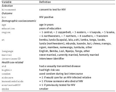
In the relevant survey, respondents are asked, at the end of their individual interview, if they would con-sent to test for HIV. If they concon-sent then a blood sample is drawn by finger prick by the interviewer, and subsequently the dried blood spot is sent to be laboratory tested for HIV. The model includes the variables described in Table 2 in the Appendix.

We specify smooth functions of all the continuous variables, and employ Markov random field smoothers to model spatial variation. All these components enter the additive predictors for the selection and HIV status equations. The selection variable (exclusion restriction) isinterviewerIDand enters the first equation only. We apply a ridge penalty to the coefficients of this variable in order to account for the difficulties associated with its use (e.g.,interviewerIDcan be collinear with other independent variables since interviewers are of-ten matched to participants on the basis of some group-level characteristics such as language and ethnicity). The additive predictor for the copula parameter only depends on the Markov random field term and allows the association parameter to vary by region. See [35] for a detailed discussion of this model specification.

We first read the data-set and region shape list (hiv.polys). Then, to account for geographic clustering of HIV we store the neighborhood structure information in an objectxtwhich is then used in specification of the Gaussian Markov random filed smoother. The model is defined below. Note that the employed specification is fairly complex and it has been adopted to illustrate the flexibility of the modeling approach.

R> library(GJRM)

R> data("hiv", package = "GJRM") R> data("hiv.polys", package = "GJRM") R> xt <- list(polys = hiv.polys)

R> sel.eq <- hivconsent ~ s(age) + s(education) + s(wealth) +

+ s(region, bs = "mrf", xt = xt, k = 7) +

+ marital + std + age1sex_cat + highhiv +

+ partner + condom + aidscare +

+ knowsdiedofaids + evertestedHIV +

+ smoke + religion + ethnicity +

+ language + s(interviewerID, bs = "re")

R> out.eq <- hiv ~ s(age) + s(education) + s(wealth) +

+ s(region, bs = "mrf", xt = xt, k = 7) +

+ marital + std + age1sex_cat + highhiv +

+ partner + condom + aidscare +

+ knowsdiedofaids + evertestedHIV +

+ smoke + religion + ethnicity +

+ language

R> theta.eq <- ~ s(region, bs = "mrf", xt = xt, k = 7) R> fl <- list(sel.eq, out.eq, theta.eq)

R> bss <- gjrm(fl, data = hiv, BivD = "J90", Model = "BSS", + margins = c("probit", "probit"))

R> mean(bss$theta)

-8.459184

R> prev(bss, sw = hiv$sw, type = "naive")

Estimated prevalence (%) with 95% interval:

12.1 (11.2,13.0)

R> set.seed(1)

R> prev(bss, sw = hiv$sw, type = "univariate")

Estimated prevalence (%) with 95% interval:

12.1 (11.6,13.2)

R> prev(bss, sw = hiv$sw)

Estimated prevalence (%) with 95% interval:

22.9 (19.9,26.3)

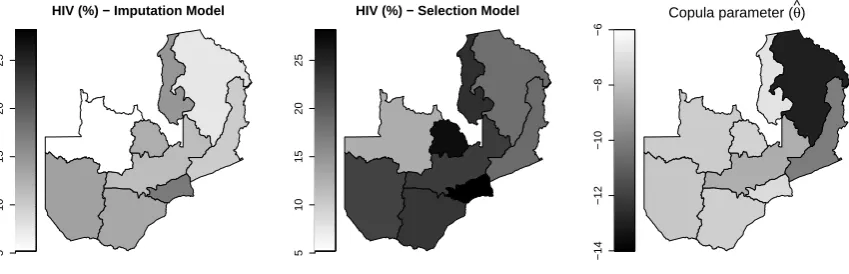
These estimates show that the selection model HIV prevalence is significantly higher than that of the imputation-based and naive models. At regional level the selection model HIV prevalences range from 13% to 28%. Note that prevalence estimates, and more generally model estimates, can be adjusted for clustering usingadjCov()oradjCovSD(). Figure 4 shows maps for the selection model and single imputation estimates as well as the dependence parameter estimates.

R> lr <- length(hiv.polys)

R> prevBYreg <- matrix(NA, lr, 2) R> thetaBYreg <- NA

R> for(i in 1:lr) {

+ prevBYreg[i,1] <- prev(bss, sw = hiv$sw, ind = hiv$region==i, type = "univariate")$res[2]

+ prevBYreg[i,2] <- prev(bss, sw = hiv$sw, ind = hiv$region==i)$res[2] + thetaBYreg[i] <- bss$theta[hiv$region==i][1]

+ }

R> zlim <- range(prevBYreg*100) # to establish a common prevalence range R> par(mfrow = c(1, 3), cex.axis = 1.3)

R> polys.map(hiv.polys, prevBYreg[,1]*100, zlim = zlim, lab = "",

+ cex.lab = 1.5, cex.main = 1.5,

+ main = "HIV (%) - Imputation Model")

R> polys.map(hiv.polys, prevBYreg[,2]*100, zlim = zlim, cex.main = 1.5, + main = "HIV (%) - Selection Model")

R> polys.map(hiv.polys, thetaBYreg, rev.col = FALSE, cex.main = 1.7,

5

10

15

20

25

HIV (%) − Imputation Model

5

10

15

20

25

HIV (%) − Selection Model

−14

−12

−10

−8

−6

Copula parameter (θ^)

Figure 4:HIV prevalence estimates by region obtained by applying the imputation and sample selection models. The copula parameter plot reports the values of the estimated associations with range_{(−∞, −1)}in the₉₀◦_{Joe copula. The higher the}

ab-solute value, the stronger the association between the selection and outcome equations.

Intervals for theθican extracted using the summary function. For instance,

R> set.seed(1)

R> CItheta <- summary(bss)$CItheta R> CItheta[1,]

2.5% 97.5%

-17.916304 -4.264049

5.3 Determinants of civil war onset

To highlight the benefits of using a bivariate probit model with partial observability, we re-estimate the model proposed in the [14]’s seminal study on civil war onset which has also been analyzed more recently by [39].

Civil wars are often theorized as the outcome of an interaction between an opposition group and the government [12, 14]. This means that we can only observe their joint decision (war onset) rather than the decisions of the single decision-makers (the opposition ‘challenges’ and the state ‘fights’). The study by [14] aims at identifying the variables that increase the likelihood of civil war onset, however cannot distinguish between variables that drive local populations to rebel against the government and variables that influence government’s fight. As in [39], the model includes the variables described in Table 3 in the Appendix.

We specify two equations, fit the model and check that convergence has been achieved.

R> library(GJRM)

R> data("war", package = "GJRM")

R> reb.eq <- onset ~ instab + oil + warl + lpopl + lmtnest +

+ ethfrac + polity2l + s(gdpenl) + s(relfrac)

R> gov.eq <- onset ~ instab + oil + warl + ncontig + nwstate + s(gdpenl)

R> bpo <- gjrm(list(reb.eq, gov.eq), data = war, Model = "BPO", margins = c("probit","probit") )

R> conv.check(bpo)

Trust region iterations before smoothing parameter estimation: 20 Loops for smoothing parameter estimation: 2

Trust region iterations within smoothing loops: 3

The convergence diagnostics suggest that the model is perhaps too complex (the gradient is close but not equal to 0 and the condition number of the information matrix relatively large). We check the estimate ob-tained forθand interval for it.

R> set.seed(1)

R> sbpo <- summary(bpo) R> sbpo$theta; sbpo$CItheta

theta 0.05459771

2.5% 97.5%

[1,] -0.8903422 0.9390838

This result suggests that the unobservable variables influencing local populations to rebel against the gov-ernment and govgov-ernment’s decision to fight back are uncorrelated. Following [2], we can therefore simplify the model by assuming a priori thatθ= 0. This implies thatp_11i=Φ(η_1i)Φ(η_2i).

R> bpo0 <- gjrm(list(reb.eq, gov.eq), data = war,

Model = "BPO0", margins = c("probit","probit")) R> conv.check(bpo0)

Largest absolute gradient value: 0.0725329 Observed information matrix is positive definite Eigenvalue range: [0.1355123,4.740461e+13]

Trust region iterations before smoothing parameter estimation: 20 Loops for smoothing parameter estimation: 2

Trust region iterations within smoothing loops: 3

The gradient is now closer to zero. However, looking at the summary results (below) one notes that the esti-mated smooth functions haveedf = 1. Hence,gdpenlandrelfraccan in principle enter the model para-metrically; this is what makes the condition number large in this case.

R> summary(bpo0)

COPULA: Gaussian MARGIN 1: Bernoulli MARGIN 2: Bernoulli

EQUATION 1

Link function for mu.1: probit

Formula: onset ~ instab + oil + warl + lpopl + lmtnest + ethfrac + polity2l + s(gdpenl) + s(relfrac)

Parametric coefficients:

oil 1.074245 0.470581 2.283 0.02244 * warl -0.598469 0.320963 -1.865 0.06224 .

lpopl 0.116009 0.045151 2.569 0.01019 *

lmtnest 0.111640 0.043090 2.591 0.00957 ** ethfrac 0.085478 0.196891 0.434 0.66419 polity2l 0.010101 0.008683 1.163 0.24471

---Signif. codes: 0 ‘***’ 0.001 ‘**’ 0.01 ‘*’ 0.05 ‘.’ 0.1 ‘ ’ 1

Smooth components’ approximate significance: edf Ref.df Chi.sq p-value

s(gdpenl) 1 1 13.763 0.000207 *** s(relfrac) 1 1 0.565 0.452208

---Signif. codes: 0 ‘***’ 0.001 ‘**’ 0.01 ‘*’ 0.05 ‘.’ 0.1 ‘ ’ 1

EQUATION 2

Link function for mu.2: probit

Formula: onset ~ instab + oil + warl + ncontig + nwstate + s(gdpenl)

Parametric coefficients:

Estimate Std. Error z value Pr(>|z|) (Intercept) -0.4317 0.6604 -0.654 0.513

instab 0.8721 0.6107 1.428 0.153

oil -0.9638 0.6070 -1.588 0.112

warl 0.2113 0.6875 0.307 0.759

ncontig 0.5862 0.4968 1.180 0.238

nwstate 2.6507 2.6739 0.991 0.322

Smooth components’ approximate significance: edf Ref.df Chi.sq p-value

s(gdpenl) 1 1 0.434 0.51

n = 6326 total edf = 17

For comparison, usingmgcv, we also fit a probit model where the joint decision of the opposition group and of the government is modeled without distinguishing between the opposition’s challenge and the government’s decision to fight back.

R> war.eq <- onset ~ instab + oil + warl + ncontig + nwstate + lpopl +

+ lmtnest + ethfrac + polity2l + s(gdpenl) + s(relfrac)

R> Probit <- gam(war.eq, family = binomial(link = "probit"), data = war) R> summary(Probit)

Family: binomial Link function: probit

Formula:

ethfrac + polity2l + s(gdpenl) + s(relfrac)

Parametric coefficients:

Estimate Std. Error z value Pr(>|z|) (Intercept) -3.641277 0.294255 -12.375 < 2e-16 *** instab 0.261447 0.100910 2.591 0.009573 **

oil 0.363108 0.122069 2.975 0.002934 **

warl -0.378155 0.129964 -2.910 0.003618 ** ncontig 0.155754 0.121656 1.280 0.200446 nwstate 0.759497 0.163264 4.652 3.29e-06 *** lpopl 0.104802 0.031235 3.355 0.000793 *** lmtnest 0.091518 0.034332 2.666 0.007684 ** ethfrac 0.078613 0.157390 0.499 0.617443 polity2l 0.009303 0.007004 1.328 0.184115

---Signif. codes: 0 ’***’ 0.001 ’**’ 0.01 ’*’ 0.05 ’.’ 0.1 ’ ’ 1

Approximate significance of smooth terms: edf Ref.df Chi.sq p-value s(gdpenl) 1.002 1.004 22.845 1.8e-06 *** s(relfrac) 1.001 1.002 0.366 0.546

---Signif. codes: 0 ’***’ 0.001 ’**’ 0.01 ’*’ 0.05 ’.’ 0.1 ’ ’ 1

R-sq.(adj) = 0.0314 Deviance explained = 10.5% UBRE = -0.845 Scale est. = 1 n = 6326

Although both the probit and bivariate probit models recover coefficients with the same signs, there are sev-eral differences in the statistical significance of these parameters (nwstate,instab, for example). What is of greater consequence, however, is that, unlike probit, the partial observability model allows for a more nu-anced separation of alternative theoretical mechanisms. For instance,instab,oilandwarlare all statisti-cally significant in the probit model; each of these variables may affect the onset of civil war through the two theoretical mechanisms, associated with opposition and government. The partial observability model per-mits for evaluating each of the player-specific and outcome-specific theoretical components. To demonstrate this point, let us focus, for instance, on how the two models separate the competing mechanisms linking civil war and GDP per capita. The probit model shows thatgdpenlhas a negative linear and statistically significant effect. The effect is linear becauseedf= 1 and has a negative impact as illustrated below.

R> coef(Probit)[(which(names(coef(Probit)) == "s(gdpenl).9"))]

s(gdpenl).9 -0.58988

(When using thin plate regression splines with basis dimensions equal to 10 and second-order penalties, if

edf= 1 then the coefficient of the ninth spline basis corresponds to the parametric linear effect.) While this

as GDP per capita increases, potential rebel groups are less likely to challenge the government. In contrast, gdpenlis not significant in government’s fight back equation.

R> coef(bpo0)[(which(names(coef(bpo)) == "s(gdpenl).9"))]

s(gdpenl).9 s(gdpenl).9 -0.9214988 0.4603390

Figure 5 displays the predicted probabilities of several outcomes (war onset, rebels challenging the state, and government fighting back) across varying values in GDP per capita.

0 2 4 6 8

0.0

0.1

0.2

0.3

0.4

0.5

Probabilities for All Outcomes

GDP per Capita (in thousands)

Pr(Outcome)

Figure 5:The probabilities of civil war predicted from the probit model are depicted as a continuous gray line. The probabilities of rebels challenging the state, of government fighting back, and of civil war from the partial observability model are depicted as dashed, dotted and continuous black lines, respectively. Note that the probabilities of civil war for both models can not be distinguished as in this case they are nearly identical.

R> probitW <- bpoW <- bpoReb <- bpoGov <- NA R> gdp.grid <- seq(0, 8)

R> median.values <- data.frame(t(apply(war, 2, FUN = median))) R> for (i in 1:length(gdp.grid)){

+ eta2 <- predict(bpo0, eq = 2, newd)

+ probitW[i] <- predict(Probit, newd, type = "response") + bpoW[i] <- pnorm(eta1)*pnorm(eta2)

+ bpoReb[i] <- pnorm(eta1) + bpoGov[i] <- pnorm(eta2) + }

R> plot(gdp.grid, probitW, type = "l", ylim = c(0, 0.55), lwd = 2, + col = "grey", xlab = "GDP per Capita (in thousands)",

+ ylab = "Pr(Outcome)", main = "Probabilities for All Outcomes", + cex.main = 1.5, cex.lab = 1.3, cex.axis = 1.3)

R> lines(gdp.grid, bpoW, lwd = 2)

R> lines(gdp.grid, bpoReb, lwd = 2, lty = 2) R> lines(gdp.grid, bpoGov, lwd = 2, lty = 3)

The probit and partial observability models yield identical results as far as the probability of civil war is concerned. However, the partial observability model reveals additional information about the effect of GDP per capita on the rebel-government interaction, by also allowing to estimate the probabilities of rebels chal-lenging the state and government fighting back. We see, for example, that while the former decreases as GDP per capita increases, the latter increases.

6 Discussion

We described the bivariate binary models implemented in theRadd-on packageGJRMand illustrated them using three case studies in which the issues of endogeneity, non-random sample selection and partial observ-ability were prevalent. The framework allows the user to specify flexibly covariate effects and the dependence structure between the margins. Given the modular structure of the estimation algorithm, other copulae and link functions can be incorporated in the package with little programming work.

Since link functions other than the ones implemented in the package may be plausible in applications, we explored the empirical performance of skew probit links, derived from the standard skew-normal distribution by [3], and power probit and reciprocal power probit links [6]. We opted for these links as they include the probit as special case and have desirable mathematical properties. We found that the use of these approaches causes numerical difficulties, which is in line with the arguments of [4]. Moreover, even when numerical convergence is achieved, the empirical results are virtually identical to those obtained when assuming probit links. We also considered non-exchangeable copulae and, following the approach detailed in [16], assessed the feasibility of usingCκ1,κ2(u,v) =u1−κ1v1−κ2C(uκ1,vκ2), 0 < κ1,κ2 < 1 in the context of bivariate binary

data. We encountered the same issues mentioned above, even when employing models with a small number of covariates and without nonlinear effects.

Appendix - Variable definitions

Table 1:MEPS data: description of the outcome and treatment variables, and observed confounders.

Variable Definition

Outcome

visits.hosp = 1at least one visit to hospital outpatient departments Treatment

private = 1private health insurance

Demographic-socioeconomic

age age in years

gender = 1male

race = 2white,= 3black,= 4native American,= 5others

education years of education

income income (000’s)

region = 2northeast,= 3mid-west,= 4south,= 5west Health-related

health = 5excellent,= 6very good,= 7good,= 8fair,= 9poor

bmi body mass index

diabetes = 1diabetic

hypertension = 1hypertensive

hyperlipidemia = 1hyperlipidemic

limitation = 1health limits physical activity

Table 2:HIV data: description of the outcome and selection variables, and observed confounders.

Variable Definition

Selection

hivconsent consent to test for HIV

Outcome

hiv HIV positive

Demographic-socioeconomic

age age in years

education years of education

region = 1central,= 2copperbelt,= 3eastern,= 4luapula,= 5lusaka, = 6northwestern,= 7northern,= 8southern,= 9western

et bemba, lunda (luapula), lala, ushi, lamba, tonga, luvale, lunda (northwestern), mbunda, kaonde, lozi, chewa, nsenga, ngoni, mambwe, namwanga, tumbuka, other

language English, Bemba, Lozi, Nyanja, Tonga, other

marital never married, currently married, formerly married

interviewerID interviewer identifier Health sex-related

std had a sexually transmitted disease

highhiv had high risk sex

condom used condom during last intercourse

aidscare = 1 if would care for an HIV-infected relative

knowsdiedofaids = 1 if know someone who died of HIV

evertestedHIV = 1 if previously tested for HIV

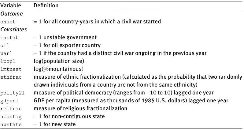
Table 3:Civil war data: description of the outcome variable and covariates.

Variable Definition Outcome

onset = 1for all country-years in which a civil war started Covariates

instab = 1unstable government

oil = 1for oil exporter country

warl = 1if the country had a distinct civil war ongoing in the previous year

lpopl log(population size)

lmtnest log(%mountainous)

ethfrac measure of ethnic fractionalization (calculated as the probability that two randomly drawn individuals from a country are not from the same ethnicity)

polity2l measure of political democracy (ranges from−10to10) lagged one year

gdpenl GDP per capita (measured as thousands of 1985 U.S. dollars) lagged one year

relfrac measure of religious fractionalization

ncontig = 1for non-contiguous state

nwstate = 1for new state

Acknowledgement: We would like to thank Bear F. Braumoeller for suggesting the implementation of the

bivariate probit model with partial observability, and a reviewer for pointing out various corrections which have improved the readability and message of the article.

References

[1] Abadie, A., D. Drukker, J. L. Herr, and G. W. Imbens (2004). Implementing matching estimators for average treatment effects in Stata.Stata J. 4(3), 290–311.

[2] Abowd, J. M. and H. S. Farber (1982). Job queues and the union status of workers.Ind. Labor. Relat. Rev. 35(3), 354–367. [3] Azzalini, A. (1985). A class of distributions which includes the normal one.Scand. J. Stat. 12(2), 171–178.

[4] Azzalini, A. and R. B. Arellano-Valle (2013). Maximum penalized likelihood estimation for skew-normal and skew-t distribu-tions.J. Stat. Plan. Infer. 143(2), 419–433.

[5] Bärnighausen, T., J. Bor, S. Wandira-Kazibwe, and D. Canning (2011). Correcting HIV prevalence estimates for survey non-participation using Heckman-type selection models.Epidemiology 22(1), 27–35.

[6] Bazan, J. L., H. Bolfarinez, and M. B. Branco (2010). A framework for skew-probit links in binary regression.Commun. Stat. Simulat. 39(4), 678–697.

[7] Buchmueller, T. C., K. Grumbach, R. Kronick, and J. G. Kahn (2005). The effect of health insurance on medical care utilization and implications for insurance expansion: a review of the literature.Med. Care Res. Rev. 62(1), 3–30.

[8] Cappellari, L. and S. P. Jenkins (2003). Multivariate probit regression using simulated maximum likelihood. Stata J. 3(3), 278–294.

[9] Chen, G. G. and T. Åstebro (2012). Bound and collapse bayesian reject inference for credit scoring.J. Oper. Res. Soc. 63(10), 1374–1387.

[10] Chib, S. and E. Greenberg (2007). Semiparametric modeling and estimation of instrumental variable models. J. Comput. Graph. Stat. 16(1), 86–114.

[11] Clarke, P. S. and F. Windmeijer (2012). Instrumental variable estimators for binary outcomes. J. Amer. Statist. Assoc. 107, 1638–1652.

[12] Collier, P. and A. Hoeffler (2004). Greed and grievance in civil war.Oxford Econ. Pap. 56, 563–595.

[13] Dubin, J. A. and D. Rivers (1989). Selection bias in linear regression, logit and probit models.Sociol. Method Res. 18(2–3), 360–390.

[14] Fearon, J. D. and D. D. Laitin (2003). Ethnicity, insurgency, and civil war.Am. Polit. Sci. Rev. 97(1), 75–90.

[15] Fitzmaurice, G., M. Davidian, G. Verbeke, and G. Molenberghs (2008). Longitudinal Data Analysis. Chapman & Hall/CRC, London.