Nonlinear Regression Estimation Using Subset-Based Kernel Principal Components

This is a repository copy of

Nonlinear Regression Estimation Using Subset-Based Kernel

Principal Components

.

White Rose Research Online URL for this paper:

http://eprints.whiterose.ac.uk/122673/

Version: Accepted Version

Article:

Ke, Yuan, Li, Degui orcid.org/0000-0001-6802-308X and Yao, Qiwei (2018) Nonlinear

Regression Estimation Using Subset-Based Kernel Principal Components. Statistica

Sinica. pp. 2771-2794. ISSN 1017-0405

Reuse

Items deposited in White Rose Research Online are protected by copyright, with all rights reserved unless

indicated otherwise. They may be downloaded and/or printed for private study, or other acts as permitted by

national copyright laws. The publisher or other rights holders may allow further reproduction and re-use of

the full text version. This is indicated by the licence information on the White Rose Research Online record

for the item.

Takedown

If you consider content in White Rose Research Online to be in breach of UK law, please notify us by

NONLINEAR REGRESSION ESTIMATION USING

SUBSET-BASED KERNEL PRINCIPAL

COMPONENTS

Yuan Ke

, Degui Li

, Qiwei Yao

1

_{Princeton University,}

_{The University of York,}

_{London School of Economics}

function. The numerical studies including three simulated examples and two real data sets illustrate the reliable performance of the proposed method. In particular, the improvement over the global KPCA method is evident.

Key words and phrases: Conditional distribution function, eigenanalysis, kernel Gram matrix, KPCA, mean regression function, nonparametric regression.

1

Introduction

LetY be a scalar response variable andX_{be ap-dimensional random vector. We are interested}

in estimating the conditional mean regression function defined by

h_px_{q “EpY|}X_“x_q, x_PG, (1.1)

techniques may result in systematic biases in estimation. For instance, the estimation based on an additive model may perform poorly when the data generation process deviates from the additive assumption.

In this paper we propose a data-driven dimension reduction approach through using a

Kernel Principal Components Analysis (KPCA) for the random covariateX_{. The KPCA is a}

nonlinear version of the standard linearPrincipal Component Analysis (PCA)and overcomes the limitations of the linear PCA by conducting the eigendecomposition of the kernel Gram matrix, see, for example, Sch¨olkopf, Smola and M¨uller (1999), Braun (2005) andBlanchard, Bousquet and Zwald(2007). See also Section2.2below for a detailed description on the KPCA and its relation to the standard PCA. The KPCA has been applied in, among others, feature ex-traction and de-noising in high-dimensional regression (Rosipalet al.,2001), density estimation (Girolami,2002), robust regression (Wibowo and Desa, 2011), conditional density estimation (Fu, Shih and Wang,2011;Izbicki and Lee,2013), and regression estimation (Lee and Izbicki,

2013).

Unlike the existing literature on KPCA, we approximate the mean regression h_px_{q on}

different subsets of the sample space of X _{by linear combinations of different subset-based}

kernel principal components. The subset-based KPCA identifies nonlinear eigenfunctions in a subset, and thus reflects the relationship betweenY and X _{on that set more parsimoniously}

than, for example, a global KPCA (see Proposition 1 in Section2.2below). The subsets may be defined according to some characteristics ofX_{and/or those on the relationship betweenY}

andX_{(e.g., MACD for financial prices, different seasons/weekdays for electricity consumption,}

observations in the present paper are collected from a strictly stationary and weakly dependent process, which relaxes the independence and identical distribution assumption in the KPCA literature and makes the proposed methodology applicable to the time series data. Under some regularity conditions, we show that the estimated eigenvalues and eigenfunctions which are constructed through an eigenanalysis on the subset-based kernel Gram matrix are consistent. The conditional mean regression functionhp¨qis then estimated through the projection to the kernel spectral space which is spanned by a few estimated eigenfunctions whose number is determined by a simple ratio method. The developed conditional mean estimation is shown to be uniformly consistent over the subset with a convergence rate faster than those of some well-known nonparametric estimation methods. We further extend the subset-based KPCA method to estimation of the conditional distribution function:

FY|Xpy|xq “PpY ďy|X“xq, xPG, (1.2)

and establish the associated asymptotic property.

2

Methodology

Let _tpYi,Xiq,1 ď i ď nu be observations from a strictly stationary process with the same

marginal distribution as that of _pY,X_{q. Our aim is to estimate the mean regression function}

hpx_{q for}x_P G, as specified in (1.1). We first introduce the kernel spectral decomposition in Section2.1, followed by the illustration on the kernel feature space and the relationship between the KPCA and the standard PCA in Section2.2, and finally propose an estimation method for the conditional mean regression function in Section2.3.

2.1

Kernel spectral decomposition

Let L2pGq be the Hilbert space consisting of all the functions defined on G which satisfy the following conditions: for anyfPL2pGq,

ż

G

fpx_qPXpdxq “E “

fpX_qIpX_PG_q‰_“0,

and

ż

G

f2px_qPXpdxq “E “

f2pX_qIpX_PG_q‰_{ă 8},

wherePXp¨qdenotes the probability measure ofX, andIp¨qis an indicator function. The inner

product onL2pGqis defined as

xf, gy “

ż

G

fpx_qgpx_qPXpdxq “CovtfpXqIpXPGq, gpXqIpXPGqu, f, gPL2pGq. (2.1)

pi, j_q-th element is non-negative definite. For any fixedu_PG,K_px_,u_{qcan be seen as a function}

ofx_{. A Mercer kernelKp¨,¨qdefines an operator on}L2pGqas follows:

fpx_{q Ñ}

ż

G

Kpx_,u_qfpu_qPXpduq.

It follows from Mercer’s Theorem (Mercer, 1909) that a Mercer kernel admits the following spectral decomposition:

Kpu_,v_{q “} d ÿ

k“1

λkϕkpuqϕkpvq, u,vPG, (2.2)

where λ1 ěλ2 ě ¨ ¨ ¨ ěλd ą0 are the positive eigenvalues of Kp¨,¨q, andϕ1, ϕ2,¨ ¨ ¨ are the orthonormal eigenfunctions in the sense that

ż

G

Kpx_,u_qϕkpu_qPXpduq “λkϕkpxq, xPG, (2.3)

and

xϕi, ϕjy “ ż

G

ϕipuqϕjpuqPXpduq “ $ ’ ’ & ’ ’ %

1 i_“j,

0 i‰j.

(2.4)

As we can see from the spectral decomposition (2.2),d_“max_tk:λką0uand is possible

to be infinity. We say that the Mercer kernel is of finite-dimension when d is finite, and of infinite-dimension whend_{“ 8}. To simplify the discussion, in this section and Section3below, we assume d is finite. This restriction will be relaxed in Section 4. We refer toFerreira and Menegatto(2009) for Mercer’s Theorem for metric spaces. The eigenvaluesλkand the associated

we construct the sample eigenvalues and eigenvectors through an eigenanalysis of the kernel Gram matrix which is defined in (2.6) below, and then obtain the estimate of the eigenfunction

ϕkby the Nystr¨om extension (Drineas and Mahoney,2005).

Define

pYjG,X G

jq, j“1,¨ ¨ ¨, m (

“ pYi,Xiq ˇ

ˇ1_ďi_ďn, X_iPG(, (2.5)

where m is the number of observations satisfying X_{i P}G, and define the subset-based kernel Gram matrix:

K_G“

¨ ˚ ˚ ˚ ˚ ˚ ˚ ˚ ˚ ˚ ˚ ˚ ˝

KpXG

1,X

G

1q KpX

G

1,X

G

2q ¨ ¨ ¨ KpX

G

1,X

G mq

K_pXG

2,X

G

1q KpX

G

2,X

G

2q ¨ ¨ ¨ KpX

G

2,X

G mq

..

. ... . .. ...

KpXG_m,XG

1q KpX

G m,X

G

2q ¨ ¨ ¨ KpX

G m,X

G mq ˛ ‹ ‹ ‹ ‹ ‹ ‹ ‹ ‹ ‹ ‹ ‹ ‚ . (2.6)

Let pλ1 ě ¨ ¨ ¨ ě λpm ě0 be the eigenvalues of KG, and ϕp₁,¨ ¨ ¨,ϕpm be the corresponding m

orthonormal eigenvectors. Write

p

ϕk“ “

p

ϕkpX G

1q,¨ ¨ ¨,ϕpkpX G mq

‰T

. (2.7)

We next use the so-called Nystr¨om extension to obtain the estimate of the eigenfunction. The Nystr¨om method is originally introduced to get the approximate numerical solution of an integral equation by replacing the integral with a representative weighted sum. The integral in (2.3) can be approximated by 1

m

řm

i“1Kpx,X

G

iqϕkpXGiq. Under some mild conditions (e.g.,

Assumption 3 in Section 3), and using the Law of Large Numbers, such an approximation is sensible. Hence, the eigenfunctionϕkpxqcan be approximated by _mλ1_k

řm

i“1Kpx,X

G

Replacingλk andϕkpXGiq bypλk{mand?mϕpkpXGiq, respectively, we may define the Nystr¨om

extension of the eigenvectorϕpkas

r

ϕkpxq “

?_m

p

λk

¨

m ÿ

i“1

Kpx_,XG iqϕpkpX

G

iq, xPG, k“1,¨ ¨ ¨, d. (2.8)

Let

r

λk“pλk{m, k“1,¨ ¨ ¨, d. (2.9)

Proposition 3 in Section 3 below shows that, for any x _P G, rλk and ϕrkpxq are consistent

estimators ofλkandϕkpxq, respectively.

Another critical issue in practical application is to estimate the dimension of the Mercer kernelKp¨,¨q. When the dimension ofKp¨,¨qisdandd!m, we may estimatedby the following ratio method (Lam and Yao,2012):

p

d_“ arg min 1ďkďtmc0u

p

λk`1{pλk“ arg min

1ďkďtmc0u

r

λk`1{rλk, (2.10)

where c0 P p0,1q is a pre-specified constant such asc0 “0.5 andtzudenotes the integer part of the numberz. The numerical results in Sections5and6show that this ratio method works well in finite sample cases.

2.2

Kernel feature space and KPCA

LetM_pKqbe ad-dimensional linear space spanned by the eigenfunctionsϕ1,¨ ¨ ¨, ϕd, and

By the spectral decomposition (2.2), M_pK_q can also be viewed as a linear space spanned by functions gup¨q ” Kp¨,uq for all u P G. Thus we call MpKq the kernel feature space as it

consists of the feature functions extracted by the kernel functionKp¨,¨q, and callϕ1,¨ ¨ ¨, ϕdthe

characteristic features determined byK_p¨,_¨qand the distribution of X _{on set}G. In addition, we callϕ1pXq, ϕ2pXq,¨ ¨ ¨ the kernel principal components ofXon setG, and one can see they are nonlinear functions ofX_{in general. We next give an interpretation to see how the KPCA}

is connected to the standard PCA.

Anyf_PM_pK_qwhose mean is zero on setG admits the following expression:

fpx_{q “} d ÿ

j“1

xf, ϕjyϕjpxq forxPG.

Furthermore,

||f_||2 _{” x}f, f_{y “}Var f_pX_qIpX_PG_q(_“ d ÿ

j“1

xf, ϕjy2.

Now we introduce a generalized variance incited by the kernel functionKp¨,¨q:

VarKtfpXqIpXPGqu “ d ÿ

j“1

λjxf, ϕjy2, (2.11)

where λj is assigned as the weight on the “direction” ofϕj forj“1, ¨ ¨ ¨ , d. Then it follows

from (2.2) and (2.3) that

ϕ1 “ arg max

fPMpKq,||f||“1

ż

GˆG

fpu_qfpv_qKpu_,v_qPXpduqPXpdvq

“ arg max

fPMpKq,||f||“1

d ÿ

j“1

λjxf, ϕjy2

“ arg max

fPMpKq,||f||“1VarKtfp

which indicates that the functionϕ1is the “direction” which maximizes the generalized variance VarKtfpXqIpXPGqu. Similarly it can be shown thatϕkis the solution of the above

maximiza-tion problem with addimaximiza-tional constraints_xϕk, ϕjy “0 for 1ďjăk. Hence, the kernel principal

components are the orthonormal functions in the feature spaceM_pK_qwith the maximal kernel induced variances defined in (2.11). In other words, the kernel principal componentsϕ1, ϕ2,¨ ¨ ¨ can be treated as “directions” while their corresponding eigenvaluesλ1, λ2,¨ ¨ ¨ can be considered as the importance of these “directions”.

A related but different approach is to viewM_pK_qas a reproducing kernel Hilbert space, for which the inner product is defined different from (2.1) to serve as a penalty in estimating functions via regularization; see section 5.8 of Hastie, Tibshirani and Friedman (2009) and Wahba(1990). Since the reproducing property is irrelevant in our context, we adopt the more natural inner product (2.1). For the detailed interpretation of KPCA in a reproducing kernel space, we refer to section 14.5.4 ofHastie, Tibshirani and Friedman(2009).

We end this subsection by stating a proposition which shows that the smaller G is, the lower the dimension ofM_pK_q is. This indicates that a more parsimonious representation can be obtained by using the subset-based KPCA instead of the global KPCA. The proof of the proposition follows immediately from (2.2) and Proposition 2 in Section2.3below.

Proposition 1. LetG¯be a measurable subset of the sample space ofX_{such that}G_ĂG¯, and

2.3

Estimation for conditional mean regression

For the simplicity of presentation, we assume that the mean of random variateh_pX_{q “EpY|}X_q

on setGis 0, i.e.

ErhpX_qIpX_PG_{qs “ErEp}Y|X_qIpX_PG_{qs “Er}Y IpX_PG_{qs “}0.

This amounts to replacing YG

i byY

G i ´Y¯

G

in (2.5) with ¯YG

“ m´1ř_1ďjďmY G

j . In general M_pK_qis a genuine subspace ofL2pGq. Suppose that on setG, hpxq “EpY|X“xq PMpKq, i.e.,hpx_{qmay be expressed as}

h_px_{q “}

ż

yfY|Xpy|xqdy“

d ÿ

k“1

βkϕkpxq, xPG, (2.12)

wherefY|Xp¨|xqdenotes the conditional density function ofY givenX“x, and

βk“ xϕk, hy “ ż

x_PG

ϕkpxqPXpdxq ż

yfY|Xpy|xqdy“ErY ϕkpXqIpXPGqs.

This leads to the estimator forβkwhich is constructed as

r

βk“

1

m

m ÿ

i“1

YiGϕrkpX G

where _pYG i ,X

G

iq,i“1,¨ ¨ ¨, m, are defined in (2.5), andϕrkp¨qare given in (2.8). Consequently

the estimator forhp¨qis defined as

r

hpx_{q “} d ÿ

k“1

r

βkϕrkpxq, xPG. (2.14)

When the dimension of the kernel Kp¨,¨q is unknown, the sum on the right hand side of the above expression runs fromj_“1 todpwithdpdetermined via (2.10).

The estimator in (2.14) is derived under the assumption that on set G, h_px_{q P} M_pK_q. When this condition is unfulfilled, (2.14) is an estimator for the projection of hp¨qonM_pKq. Hence the goodness ofrhp¨qas an estimator forhp¨qdepends critically on (i) kernel functionK, (ii) set G and PXp¨qonG. In the simulation studies in Section 5below, we will illustrate an

approach to specifyG. Ideally we would like to choose a Kp¨,¨qthat induces a large enough

M_pK_qsuch thath_PM_pK_q. Some frequently used kernel functions include

• Gaussian kernel: Kpu_,v_{q “expp´||}u_´v_||2_{cq,

• Thin-plate spline kernel: K_pu_,v_{q “ ||}u_´v_||2_logp||u_´v_||q,

• Polynomial kernel (Fu, Shih and Wang,2011):

K_pu_,v_{q “}

$ ’ ’ & ’ ’ %

r1_{´ p}u1v_qℓ`1_s{p1´u1v_{q, if}u1v_‰1,

ℓ`1, otherwise,

where _{|| ¨ ||}denotes the Euclidean norm,cis a positive constant, and ℓ_ě1 is an integer. Also note that for any functions inψ1,¨ ¨ ¨, ψdPL2pGq,

Kpu_,v_{q “} d ÿ

k“1

is a well-defined Mercer kernel. A possible choice of the kernel function is to let_tψ1puq,¨ ¨ ¨ , ψdpuqu

be a set of basis functions ofu_{, e.g., Fourier series, polynomial series, wavelets, B-spline, etc.}

The numerical studies in Sections5and6use (2.15) with appropriately chosen functionsψkin

the estimation and dimension reduction procedure, which performs reasonably well. The follow-ing proposition shows that the dimension ofM_pKq withKp¨,¨q defined above is controlled by

d.

Proposition 2. For the kernel functionKp¨,¨qdefined in (2.15), dim_tM_pKqu ďd.

3

Large sample theory

In this section, we study the asymptotic properties for the estimators of the eigenvalues and eigenfunctions of the Mercer kernel as well as the mean regression estimation. We start with some regularity conditions which are sufficient to derive our asymptotic theory.

Assumption 1_{.The processtpYi,}X_{iquis strictly stationary andα-mixing (or strongly mixing)} dependent with the mixing coefficient satisfying

αt“Opt´κq, κą2δ˚`p`3

2, (3.1)

wherepis the dimension of the random covariate,0ďδ˚ă 8such that the volume of

the setG has the ordermδ˚_.

Assumption 2.The positive eigenvalues of the Mercer kernelKp¨,¨qare distinct and satisfy

Assumption 3_{.The eigenfunctions ϕj,j “1,¨ ¨ ¨, d, are Lipschitz continuous and bounded} on the setG. Furthermore, the kernel Kp¨,x_{q is Lipschitz continuous and bounded on}

the setG for anyx_PG.

Remark 1_{. In Assumption 1, we allow the process to be stationary andα-mixing dependent,}

which is mild and can be satisfied by some commonly-used time series models; see e.g., Section 2.6 ofFan and Yao(2003) and the references within. For example the causal ARMA processes with continuous innovations areα-mixing with exponentially decaying mixing coefficients. Note that for the processes with exponentially decaying mixing coefficients, (3.1) is fulfilled automat-ically, and the technical arguments in the proofs can be simplified. We allow setG to expand with the size of the sub-sample in G in the order of mδ˚_{, andδ}

˚ would be 0 ifG is bounded.

Assumptions 2 and 3 impose mild restrictions on the eigenvalues and eigenfunctions of the Mer-cer kernel, respectively. They are crucial to ensure the consistency of the sample eigenvalues and eigenvectors constructed in Section2.1. The boundedness condition onϕj and Kp¨,xqin

Assumption 3 can be replaced by the 2_p2_`δ_q-order moment conditions for someδ _ą0, and Proposition 3 below still holds at the cost of more lengthy arguments. Furthermore, by the smoothness condition on the kernel function and using (3.2) in Proposition 3 below, we may easily show thatϕrjp¨qdefined in (2.8),j“1,¨ ¨ ¨, d, are Lipschitz continuous and bounded with

probability tending to one.

Proposition 3.Suppose that Assumptions 1–3 are satisfied. Then we have

max 1ďkďd

ˇ ˇ ˇrλk´λk

ˇ ˇ

ˇ“ max

1ďkďd ˇ ˇ ˇ

ˇ_m1pλk´λk ˇ ˇ ˇ

ˇ“OP

´

m´1{2¯ (3.2)

and

max

1ďkďdsup|ϕrkp

whereξm“m´1{2log1{2m.

Remark 2_{. Proposition 3 presents the convergence rates of the estimated eigenvalues and}

eigen-functions of the Mercer kernel K_p¨,_¨q. The result is of independent interest. It complements some statistical properties of the KPCA in the literature such asBraun(2005) andBlanchard, Bousquet and Zwald(2007). Note thatPpX_PG_qcan be consistently estimated bym_{n. If it is assumed thatPpX_PG_{q “}c0ą0,mwould be of the same order as the full sample sizen(with probability tending to one). As a consequence, the convergence rates in (3.2) and (3.3) would be equivalent to OP

´

n´1{2¯ and OP ´

n´1{2log1{2n¯, respectively, which are not uncommon in the context of functional principal component analysis (Bosq,2000;Horv´ath and Kokoszka, 2012). Based on Proposition 3, we can easily derive the following uniform consistency result for

r

h_p¨q.

Theorem 1_{.Suppose that Assumptions 1–3 are satisfied, Er|Y|}2`δ

s ă 8for someδ _ą0and

hp¨q PM_pKq. Then it holds that

sup

x_PG

ˇ ˇ

ˇrhpx_{q ´hp}x_q

ˇ ˇ

ˇ“OPpξmq, (3.4)

whereξmis defined in Proposition 3.

Remark 3. As stated above, the uniform convergence rate in (3.4) is equivalent toOP ´

n´1{2log1{2_n¯_, which is faster than the well-known uniform convergence rateOP

´

pnb_q´1{2log1{2n¯in the ker-nel smoothing method (Fan and Yao,2003), wherebis a bandwidth which converges to zero as

ntends to8. The intrinsic reason of the faster rate in (3.4) is that we assume the dimension of the subset-based kernel feature space is finite, and thus the number of the unknown elements in (2.12) is also finite. Section 4below shows that the increasing dimension of the kernel feature

4

Extensions of the estimation methodology

In this section, we consider two extensions of the methodology proposed in Section 2: the estimation for the conditional distribution function, and the case when the dimension of a kernel feature space diverges together with the sample size.

4.1

Estimation for conditional distribution functions

Estimation of the conditional distribution function defined in (1.2) is a key aspect in various statistical topics (such as the quantile regression), as the conditional mean regression may be not informative enough in many situations. Nonparametric estimation of the conditional dis-tribution has been extensively studied in the literature includingHall, Wolff and Yao (1999), Hansen (2004) andHall and Yao (2005). In this section, we use the subset-based KPCA ap-proach discussed above to estimate a conditional distribution function in low-dimensional kernel feature space when the random covariates are multi-dimensional.

Let F˚py|xq “FY|Xpy|xq ´c˚, wherec˚ “PpY ďy,XPGq. ThenErF˚py|Xqs “0. In

practicec˚ can be easily estimated by the relative frequency. Suppose that F˚py|¨q PMpKq,

i.e.,

F˚py|xq “FY|Xpy|xq ´c˚“

ży

´8

fY|Xpz|xqdz´c˚“

d ÿ

k“1

βk˚ϕkpxq, xPG. (4.1)

Note that the coefficientsβk˚in the above decomposition depend on y. The orthonormality of

ϕiimplies that

β˚k “ xF˚py|¨q, ϕky “ ż

G

ϕkpxqPXpdxq

„ży

´8

fY|Xpz|xqdz´c˚ 

“

ż

I_pz_ďy,x_PG_qϕkpxqfY|Xpz|xqdzPXpdxq ´c_˚ ż

G

ϕkpxqPXpdxq

This leads to the following estimator forβk˚:

r

βk˚“

1

m

m ÿ

i“1

I_pYiGďyqϕrkpX G iq ´r

c˚

m

m ÿ

i“1

r

ϕkpX G

iq, (4.2)

where_pYiG,X G

iqare defined in (2.5),ϕrkp¨qare defined in (2.8), and

r

c˚“ 1

n

n ÿ

i“1

IpYiďy, XiPGq, (4.3)

nis the full sample size. Consequently, we obtain the estimator for the conditional distribution:

r

FY|Xpy|xq “

d ÿ

k“1

r

β˚kϕrkpxq `rc˚. (4.4)

The estimator FrY|Xp¨|xq is not necessarily a bona fide distribution function. Some further

normalization may be required to make the estimator non-negative, non-decreasing and between 0 and 1 (Glad, Hjort and Ushakov,2003).

By the classic result for the α-mixing sequence, we may show that rc˚ is a consistent

estimator ofc˚ with a root-nconvergence rate. Then, by Proposition 3 and following the proof

of Theorem 1, we have the following convergence result forFrY|Xpy|xq.

Theorem 2.Suppose that Assumptions 1–3 are satisfied andF˚py|¨q PMpKq. Then it holds

that

sup

xPG

ˇ ˇ

ˇ rFY|Xpy|xq ´FY|Xpy|xq ˇ ˇ

ˇ“OPpξmq (4.5)

4.2

Kernel feature spaces with diverging dimensions

We next consider the case when the dimension of the kernel feature spacedm”maxtk:λką0u

depends onm, and may diverge to infinity asmtends to infinity. Let

ρm“mintλk´λk`1, k“1,¨ ¨ ¨, dmu.

In order to derive a more general asymptotic theory, we need to slightly modify Assumption 2.

Assumption2˚_{.The positive eigenvalues of the Mercer kernelK}

p¨,¨qare distinct and satisfy

0_ăλdm ă ¨ ¨ ¨ ăλ2ăλ1ă 8,

řdm

k“1λkă 8.

The following proposition shows that the divergingdm would slow down the convergence

rates in Proposition 3.

Proposition 4_{.Suppose that Assumptions 1,2}˚_{and 3 are satisfied,dm“o}`_mρ2_mλ2_d

m{logm

˘

,

and theα-mixing coefficient decays to zero at an exponential rate. Then it holds that

max 1ďkďdm

ˇ ˇ ˇrλk´λk

ˇ ˇ

ˇ“ max

1ďkďdm

ˇ ˇ ˇ

ˇ_m1pλk´λk ˇ ˇ ˇ

ˇ“OP

´

d1m{2ξm ¯

(4.6)

and

max 1ďkďdm

sup

xPG|r

ϕkpxq ´ϕkpxq| “OP ´

d1m{2ξm{pρmλdmq

¯

. (4.7)

Remark 4_{. Whendm is fixed, it may be reasonable to assume bothρm andλdm are bounded}

convergence rates in (4.6) and (4.7) would be generally slower than those in (3.2) and (3.3). Let

ci,i“1, ¨ ¨ ¨ ,5, be five positive constants. For any two sequencesamandbm,am9bmmeans

that 0_ăc4ďam{bmďc5ă 8whenmis sufficiently large. Ifdm“c1logm,ρm“c2log´1m andλdm“c3log

´1_{m, we have}

d1m{2ξm9m´1{2logm, d1m{2ξm{pρmλdmq 9m

´1{2_log3

m.

Using Proposition 4 and following the proof of Theorem 1, we can easily obtain the uniform convergence rate for the conditional mean regression estimation whendmis diverging.

In practice, we may encounter the more challenging case when the dimension of the Mercer kernel is infinite (e.g.,λk 9k´ι1 withι1 ą0 orλk 9ιk2 with 0ăι2 ă1). In this case, the convergence result in Proposition 4 is not directly applicable as the rates in (4.6) and (4.7) become divergent when the dimension is infinite. However, the proposed subset-based KPCA approach can still be used to estimate the conditional mean regression function. Assuming that the mean regression functionhpx_{q P}M_pKqand noting that the dimension ofM_pKqis infinite, we have

h_px_{q “}

8 ÿ

k“1

βkϕkpxq “ dm

ÿ

k“1

βkϕkpxq `

8 ÿ

k“dm`1

βkϕkpxq ”h1pxq `h2pxq, (4.8)

where βk and ϕkpxq are defined as in Section2, anddm is a divergent number satisfying the

condition in Proposition 4. LetM1pKq be adm-dimensional kernel feature space spanned by

ϕ1,¨ ¨ ¨, ϕdm. From (4.8), the mean regression functionhpxq can be well approximated by its

some smoothness condition onh_px_{qand letdmdivergent at an appropriate rate, which is similar}

to the conditions on sieve approximation accuracy (Chen,2007). Letb‹

m“supx_PG|h2pxq|. We may estimateβkandϕk,k“1,¨ ¨ ¨, dm, in the same manner

as in Sections2.2and2.3. Denote the estimates byβrk andϕrk, and letrhmpxq “řd_km_“1βrkϕrkpxq.

By Proposition 4 and following the proof of Theorem 1, we can establish the following uniform convergence rate:

sup

x_PG

ˇ ˇ

ˇrhmpxq ´h1pxq

ˇ ˇ

ˇ“OPpνm‹q,

whereνm‹ “d3m{2ξm{pρmλdmq. Furthermore, we can prove, via the decomposition in (4.8), that

sup

x_PG

ˇ ˇ

ˇrhmpxq ´hpxq ˇ ˇ

ˇ“sup

x_PG

ˇ ˇ

ˇrhmpxq ´h1pxq

ˇ ˇ

ˇ`sup

x_PG|

h2pxq| “OPpνm‹ `b‹mq.

5

Simulation Studies

In this section, we use three simulated examples to illustrate the finite sample performance of the proposed subset-based KPCA method and compare it with the global KPCA and other existing nonparametric estimation methods, i.e., cubic spline, local linear regression and kernel ridge regression. We start with an example to assess the out-of-sample estimation performance of conditional mean function based on a multivariate nonlinear regression model. Then, in the second example, we examine the one-step ahead out-of-sample forecast performance based on a multivariate nonlinear time series model. Finally, in the third example, we examine the finite sample performance of the estimation of conditional distribution function.

as in (2.15) with_tψ1puq,¨ ¨ ¨, ψdpuqubeing a set of normalized polynomial basis functions (with

the unit norm) ofu_{“ pu1,¨ ¨ ¨, upq}T_{of order 2 and 3, i.e.,t1, uk,¨ ¨ ¨u}r

k, k“1,¨ ¨ ¨, pu, where

r “2,3 and d“rp`1. For the latter case, we call the kernel asthe quadratic kernelwhen

r _“ 2 and the cubic kernel when r _“ 3. In practice, d is estimated by the ratio method as in (2.10). The simulation results show that (2.10) can correctly estimatedp“dwith frequency close to 1. The subset is chosen to be the tκnunearest neighbors, wherenis the sample size and κ_{P p}0,1_q is a constant bandwidth. The bandwidthκand the tuning parameter cin the Gaussian kernel are selected by a 5-fold cross validation.

Example 5.1. Consider the following model:

yi“gpx2iq `sintπpx3i`x4iqu `x5i`logp1`x26iq `εi,

where x1i,¨ ¨ ¨, x6i andεi are i.i.d. Np0,1q,gpxq “e´2x

2

forx_ě0, andg_px_{q “}e´x2 _forx

ă0. In the model, the covariatex1i is irrelevant toyi.

We draw a training sample of sizen_“500 or 1000 and a testing sample of size 200. We estimate the conditional mean regression function using the training sample, and then calculate the mean squared errors (MSE) and out-of-sampleR2s over the testing sample as follows:

MSE_“ 1 200

200_ÿ

i“1

”

yi´rhpxiq ı2

, R2_“1_´

ř200

i“1ryi´rhpxiqs2

ř200

i“1pyi´y¯q2

,

whererhp¨qis defined as in (2.14),x_{i“ px1i,¨ ¨ ¨, x6iq}T_{and ¯yis the sample mean ofyiover the}

training sample.

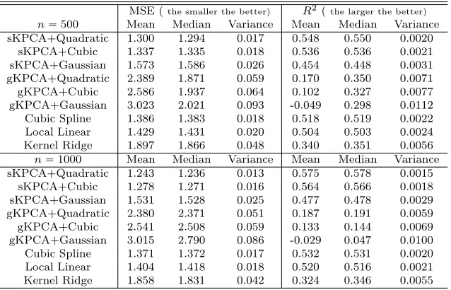
of MSE andR2. The simulation results are reported in Table 1. In this simulation, for the quadratic kernel and cubic kernel, the ratio method in (2.10) can always correctly estimate

p

d“rp`1. According to the results in Table 1, the subset-based KPCA with the quadratic kernel outperforms the global KPCA methods and other nonparametric methods as it has the smallest sample mean, median and variance of MSE and the highestR2. In addition, both the quadratic kernel and cubic kernel perform better than the Gaussian kernel due to the fact that they can better capture different degree of smoothness on different directions.

To assess the the bandwidth choice for subset-based KPCA, we set n_“ 500, letκvary from 0.05 to 0.8 and calculate the sample mean of MSE over 100 replications. The results are plotted in Figure 1. According to Figure 1, the subset-based KPCA method is not sensitive to the choice ofκ. The smallest MSE is achieved at κ_“0.27, and any κbetween 0.15 and 0.45 yields similar result.

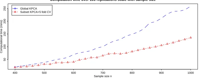
Furthermore, we compare the computational costs between the subset-based KPCA and global KPCA approaches with quadratic kernel function. The computational cost of subset-based KPCA includes the selection of bandwidth κ. The bandwidth κ is selected by 5-fold cross validation over 10 grid points equally spaced between 0.1 and 0.5. We let the sample size increase from 400 to 1000 with a step size of 20 and record the computational time over 100 replications for both approaches. The comparison results are presented in Figure 2. The major computational cost of the global KPCA methods is the eigen-decomposition of thenˆngram matrix which is of computational complexityO_pnω

q for someω_ą2. To see this, we calculate the empirical order of growth for both approaches:

p

ω“₃₀1

30

ÿ

l“1

log_pTl`1{Tlq

log_pnl`1{nlq

wherenlis thel-th component in the sett400,420,¨ ¨ ¨,980,1000uandTlis the corresponding

computational cost over 100 replications. The empirical order of growth for the global KPCA is 2.69, whereas that for the subset-based KPCA is 2.17. Hence, both Figure 2 and the calculation of empirical order of growth show the subset-based KPCA method scales with sample size much better than the global counterpart.

Table 1: Out-of-sample estimation performance in Example 5.1

MSE (the smaller the better) R2₍the larger the better)

n_{“500 Mean Median Variance Mean Median Variance}

sKPCA+Quadratic 1.300 1.294 0.017 0.548 0.550 0.0020 sKPCA+Cubic 1.337 1.335 0.018 0.536 0.536 0.0021 sKPCA+Gaussian 1.573 1.586 0.026 0.454 0.448 0.0031 gKPCA+Quadratic 2.389 1.871 0.059 0.170 0.350 0.0071 gKPCA+Cubic 2.586 1.937 0.064 0.102 0.327 0.0077 gKPCA+Gaussian 3.023 2.021 0.093 -0.049 0.298 0.0112 Cubic Spline 1.386 1.383 0.018 0.518 0.519 0.0022 Local Linear 1.429 1.431 0.020 0.504 0.503 0.0024 Kernel Ridge 1.897 1.866 0.048 0.340 0.351 0.0056 n_{“1000 Mean Median Variance Mean Median Variance}

sKPCA+Quadratic 1.243 1.236 0.013 0.575 0.578 0.0015 sKPCA+Cubic 1.278 1.271 0.016 0.564 0.566 0.0018 sKPCA+Gaussian 1.531 1.528 0.025 0.477 0.478 0.0029 gKPCA+Quadratic 2.380 2.371 0.051 0.187 0.191 0.0059 gKPCA+Cubic 2.541 2.508 0.059 0.133 0.144 0.0069 gKPCA+Gaussian 3.015 2.790 0.086 -0.029 0.047 0.0100 Cubic Spline 1.371 1.372 0.017 0.532 0.531 0.0020 Local Linear 1.404 1.418 0.018 0.520 0.516 0.0021 Kernel Ridge 1.858 1.831 0.042 0.324 0.346 0.0055

“sKPCA” and “gKPCA” stand for the subset-based KPCA and global KPCA; “Quadratic”,

“Cu-bic” and “Gaussian” stand for the quadratic kernel, cubic kernel and Gaussian kernel, respectively;

“Cubic Spline”, “Local Linear” and “Kernel Ridge” stand for non-parametric estimation methods

based on cubic spline, local linear regression and kernel ridge regression.

Example 5.2_{. Consider the following time series model:}

● ● ● ● ● ● ● ● ● ● ● ● ● ● ● ● ● ● ● ● ● ● ● ● ● ● ● ● ●

0.2 0.4 0.6 0.8

1.3

1.4

1.5

1.6

1.7

Estimation performance of subset KPCA with respect to bandwidth kappa

Bandwidth kappa

Mean of MSE o

v

er 100 replications

Figure 1: The out-of-sample estimation performance of the subset-based KPCA approach with the quadratic kernel with respect to the bandwidthκ_whenn_“500.

● ● ● ● ● ● ● ● ● ● ● ● ● ● ● ● ● ● ● ● ● ● ● ● ● ● ● ● ● ● ●

400 500 600 700 800 900 1000

50

100

150

200

250

Computation time over 100 replications scale with sample size

Sample size n

Computational time (mins)

● Global KPCA

Subset KPCA+5 fold CV

Figure 2: The computation costs for global KPCA method and subset-based KPCA method (with κ_{selected by 5-fold cross validation) with respect to the sample size.}

wherey0“0 andtǫtuis a sequence of independentNp0,1qrandom variables. We next estimate

the conditional meanEpyt|yt´1, yt´2, yt´3, yt´4qand denote the estimator aspyt which is to be

used as the one-step-ahead predictor ofyt.

k_“1,_{¨ ¨ ¨},100, we use theT observations right before timeT_`kas the training set to predict

yT`k. The performance is measured by MSE and out-of-sampleR2:

MSPE_“ 1 100

100_ÿ

k“1

pyT`k´ypT`kq2, R2“1´

ř100

k“1pyT`k´ypT`kq2

ř100

k“1pyT`k´y¯q 2 ,

where ¯yis the sample mean ofytover the training sample.

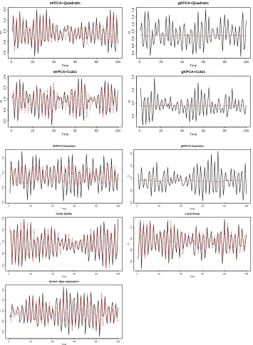
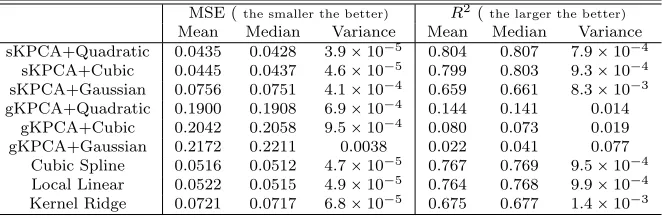
We setT “500, and repeat the experiment 200 times for each method. The sample means, medians and variances of MSE and R2 are presented in Table 2. Similar to Example 5.1, the subset-based KPCA method with the quadratic kernel provides the most accurate prediction. The subset-based KPCA method with the cubic kernel is a close second best in terms of both MSE and R2_{. Figure 3 plots a typical path together with their one-step-ahead forecasts for} each method. The typical path is the replication with median R2. Figure 3 shows that the forecasted path from the subset-based KPCA method with the quadratic kernel follows the true path closely. A similar pattern can also be found for other subset-based KPCA method with the cubic and Gaussian kernel and the three nonparametric methods (cubic spline, local linear and kernel ridge). However the global KPCA methods fail to capture the variation of the series and tend to forecast the future values by the overall mean value, which is not satisfactory.

Example 5.3.Consider the model:

X1„Np0, 1q, X2 „Np0, 1q,

Y|pX1, X2q „NpX1, 1`X22q.

The conditional distribution of Y given X _{” pX1, X2q}T _{is a normal distribution with mean}

0 20 40 60 80 100 0.0 0.5 1.0 1.5 2.0 sKPCA+Quadratic Time Yt

0 20 40 60 80 100

0.4 0.6 0.8 1.0 1.2 1.4 1.6 gKPCA+Quadratic Time Yt

0 20 40 60 80 100

0.0 0.5 1.0 1.5 2.0 sKPCA+Cubic Time Yt

0 20 40 60 80 100

0.5 1.0 1.5 2.0 gKPCA+Cubic Time Yt

0 20 40 60 80 100

0.0 0.5 1.0 1.5 sKPCA+Gaussian Time Yt

0 20 40 60 80 100

0.0 0.5 1.0 1.5 2.0 gKPCA+Gaussian Time Yt

0 20 40 60 80 100

0.0 0.5 1.0 1.5 2.0 Cubic Spline Time Yt

0 20 40 60 80 100

0.0 0.5 1.0 1.5 Local linear Time Yt

0 20 40 60 80 100

0.0

0.5

1.0

1.5

2.0

Kernel ridge regression

Time

Yt

Figure 3: One-step ahead out-of-sample forecasting performance based on the replication with medianR2 _{for each method. The black solid line is the true value and the red dashed line is the}

Table 2: One-step ahead forecasting performance in Example 5.2

MSE (the smaller the better) R2₍the larger the better)

Mean Median Variance Mean Median Variance sKPCA+Quadratic 0.0435 0.0428 3._9ˆ10´5 _{0.804 0.807 7}._9ˆ10´4

sKPCA+Cubic 0.0445 0.0437 4._6ˆ10´5 _{0.799 0.803 9}._3ˆ10´4 sKPCA+Gaussian 0.0756 0.0751 4._1ˆ10´4 _{0.659 0.661 8}._3ˆ10´3 gKPCA+Quadratic 0.1900 0.1908 6._9ˆ10´4 _{0.144 0.141 0.014}

gKPCA+Cubic 0.2042 0.2058 9._5ˆ10´4 _{0.080 0.073 0.019} gKPCA+Gaussian 0.2172 0.2211 0.0038 0.022 0.041 0.077

Cubic Spline 0.0516 0.0512 4._7ˆ10´5 _{0.767 0.769 9}._5ˆ10´4 Local Linear 0.0522 0.0515 4._9ˆ10´5 _{0.764 0.768 9}._9ˆ10´4

Kernel Ridge 0.0721 0.0717 6._8ˆ10´5 _{0.675 0.677 1}._4ˆ10´3

conditional distribution functionFY|Xpy|xqusing the subset-based KPCA with the quadratic

kernel.

We draw a training sample of size n_“300 or 500 and a testing sample of size 100. The estimated conditional distributionFrY|Xpyi|xiqis obtained using the training data. We repeat

the simulation 200 times and measure the performance by MSE as well as largest absolute error (LAE) over the testing sample:

MSE_“ 1 100

100_ÿ

i“1

” r

FY|Xpyi|xiq ´FY|Xpyi|xiq ı2

,

LAE_“ sup

py,xqPΩ˚

ˇ ˇ

ˇ rFY|Xpy|xq ´FY|Xpy|xq ˇ ˇ ˇ,

where Ω˚_{is the union of all validation sets. The results are reported in Table 3. As the values of}

Table 3: Estimation of the conditional distribution function

MSE LAE

Mean Median Variance

n_{“300 6}._0ˆ10´4 ₄._1ˆ10´4 ₃._6ˆ10´7 _0.098 n_{“500 3}._7ˆ10´4 ₂._8ˆ10´4 ₈._6ˆ10´8 _0.080

6

Real data analysis

In this section, we apply the proposed subset-based KPCA method to two real data examples. Throughout this section, the kernel function is set to be either Gaussian or Quadratic kernel. The subset is chosen to be thetκnunearest neighbors, wherenis the sample size andκP p0,1_q. The bandwidthκis selected by 5-fold cross validation.

6.1

Circulatory and respiratory problem in Hong Kong

We study the circulatory and respiratory problem in Hong Kong via an environmental data set. This data set contains 730 observations and was collected between January 1, 1994 and December 31, 1995. The response variable is the number of daily total hospital admissions for circulatory and respiratory problems in Hong Kong, and the covariates are daily measurements of seven pollutants and environmental factors: SO2, NO2, dust, temperature, change of tem-perature, humidity and ozone. We standardize the data so that all the covariates have zero sample mean and unit sample variance. To check the stationarity, we apply the augmented Dickey-Fuller test (e.g.,Dickey and Fuller,1981) to each variable in the data set. The tests are applied using the “urca” package inRand the lags included are selected by AIC. For each vari-able, the test result suggests us to reject the unit root null hypothesis. Therefore, we consider the variables in the dataset to be stationary.

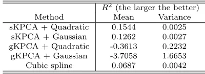
circulatory and respiratory problem using the collected environmental data, i.e., estimate the conditional mean regression function. The estimation performance is measured by the mean and variance of the out-of-sampleR2, which are calculated by a bootstrap method described as follows. We first randomly divide the data set into a training set of 700 observations and a testing set of 30 observations. For each observation in the testing set, we use the training set to estimate its conditional mean regression function. Then we calculate out-of-sample R2 for the testing set as in Example 5.1. By repeating this re-sampling and estimation procedure 1000 times, we obtain a bootstrap sample ofR2s, and calculate its sample mean and variance.

Table 4: Estimation performance for the Hong Kong environmental data

R2_{(the larger the better)}

Method Mean Variance

sKPCA + Quadratic 0.1544 0.0025 sKPCA + Gaussian 0.1262 0.0027 gKPCA + Quadratic -0.3613 0.2232 gKPCA + Gaussian -3.7058 1.6653 Cubic spline 0.0687 0.0042

6.2

Forecasting the log return of CPI

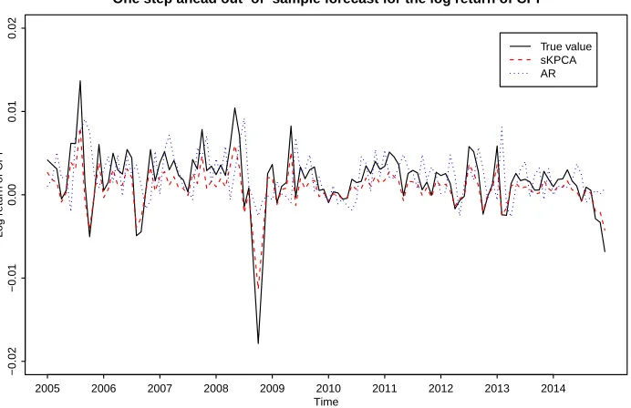
The CPI is a statistical estimate that measures the average change in the price paid to a market basket of goods and services. The CPI is often used as an important economic indicator in macroeconomic and financial studies. For example, in economics, CPI is considered as closely related to the cost-of-living index and used to adjust the income eligibility levels for government assistance. In finance, CPI is considered as an indicator of inflation and used as the deflater to translate other financial series to inflation-free ones. Hence, it is always of interest to forecast the CPI. We next perform one-step-ahead forecasting for the monthly log return of CPI in USA based on the proposed subset-based KPCA method with the quadratic kernel. The data span from January 1970 to December 2014 with 540 observations. The augmented Dickey-Fuller test suggests the monthly log return of CPI over this time span is stationary.

Instead of using the traditional linear time series models, we consider that the log return of CPI follows a nonlinear AR(3) model:

yt“gpyt´1, yt´2, yt´3q `ǫt,

wheregp¨qis an unknown function andǫtdenotes an unobservable noise at timet. The regression

functiong_p¨qis estimated by the subset-based KPCA method with the quadratic kernel. For the comparison purpose, we also forecastyt based on a linear AR(p) model with the

orderpdetermined by AIC. Suppose the testing set starts from timeT and ends at timeT_`S, the forecast performance is measured by the out-of-sampleR2as

R2_“1_´

S ř

s“1p

yT`s´ypT`sq2

S ř

s“1p

yT`s´y¯q2

whereypT`sis the estimator ofyT`s, and ¯yis the sample mean ofyt over the training set.

We set the data from January 2005 to December 2014 as the testing set, which contains 120 observations. We forecast each observation in the testing set with the data up to its previous month. The out-of-sample R2 is calculated over the testing set. The out-of-sampleR2 of the nonlinear AR(3) model is 0.2318 while theR2 of the linear AR model is 0.0412. The detailed forecasting result is plotted in Figure 4, which shows clearly that the forecast based on the subset-based KPCA method is more accurate as it captures the variations much better than the linear AR modelling method.

−0.02

−0.01

0.00

0.01

0.02

One step ahead out−of−sample forecast for the log return of CPI

Time

Log retur

n of CPI

2005 2006 2007 2008 2009 2010 2011 2012 2013 2014 True value sKPCA AR

7

Conclusion

In this paper, we have developed a new subset-based KPCA method for estimating nonparamet-ric regression functions. In contrast to the conventional (global) KPCA method which builds on a global kernel feature space, we use different lower-dimensional subset-based kernel feature spaces at different locations of the sample space. Consequently the resulting localized kernel principal components provide more parsimonious representation for the target regression func-tion, which is also reflected by the faster uniform convergence rates presented in Theorem 1, see also the discussions immediately below Theorem 1. The reported numerical results with both simulated and real data sets illustrate clearly the advantages of using the subset-based KPCA method over its global counterpart. It also outperforms some popular nonparametric regression methods such as the cubic spline and kernel regression (the results on kernel regression are not reported to save the space). It is also worth mentioning that the quadratic kernel constructed based on (2.15) using normalized univariate linear and quadratic basis functions performs better than the more conventional Gaussian kernel for all the examples reported in Sections5and6.

Supplementary materials

The online supplementary material contains the detailed proofs of Propositions 1–4 and Theorem 1.

Acknowledgements

References

Blanchard, G., Bousquet, O. and Zwald, L. (2007). Statistical properties of kernel principal component

analysis.Machine Learning,66, 259–294.

Bosq, D. (2000). Linear Processes in Function Spaces: Theory and Applications. Lecture Notes in

Statistics, Springer.

Braun, M. L. (2005).Spectral Properties of the Kernel Matrix and Their Relation to Kernel Methods

in Machine Learning. PhD Thesis, University of Bonn, Germany.

Chen, X. (2007). Large sample sieve estimation of semi-nonparametric models.Handbook of

Economet-rics,76, North Holland, Amsterdam.

Dickey, A.D. and Fuller, W. A. (1981). Likelihood ratio statistics for autoregressive time series with a

unit root.Econometrica,49_{, 1057–1072.}

Drineas, P. and Mahoney, M. (2005). On the Nystr¨om method for approximating a Gram matrix for

improved kernel-based learning.Journal of Machine Learning Research,6_{, 2153–2175.}

Ferreira, J. C. and Menegatto, V. A. (2009). Eigenvalues of integral operators defined by smooth positive

definite kernels.Integral Equations and Operator Theory,64, 61–81.

Fan, J. and Gijbels, I. (1996).Local Polynomial Modelling and Its Applications. Chapman and Hall,

London.

Fan, J. and Yao, Q. (2003).Nonlinear Time Series: Nonparametric and Parametric Methods. Springer,

New York.

Fu, G., Shih, F.Y. and Wang, H. (2011). A kernel-based parametric method for conditional density

estimation.Pattern Recognition,44_{, 284-294.}

Girolami, M. (2002). Orthogonal series density estimation and the kernel eigenvalue problem.Neural

Glad, I.K., Hjort, N.L. and Ushakov, N.G. (2003). Correction of density estimators that are not densities.

Scandinavian Journal of Statistics,30, 415-427.

Green, P. and Silverman, B. (1994). Nonparametric Regression and Generalized Linear Models: A

Roughness Penalty Approach. Chapman and Hall/CRC.

Hall, P., Wolff, R.C.L. and Yao, Q. (1999). Methods for estimating a conditional distribution function.

Journal of the American Statistical Association,94, 154-163.

Hall, P. and Yao, Q. (2005). Approximating conditional distribution functions using dimension reduction.

The Annals of Statistics,33, 1404-1421.

Hansen, B. (2004). Nonparametric estimation of smooth conditional distributions. Working paper

avail-able athttp://www.ssc.wisc.edu/„bhansen/papers/cdf.pdf.

Hastie, T., Tibshirani, R. and Friedman, J. (2009).The Elements of Statistical Learning(2nd Edition).

Springer, New York.

Horv´ath, L. and Kokoszka, P. (2012).Inference for Functional Data with Applications. Springer Series

in Statistics.

Izbicki, R. and Lee, A.B. (2013). Nonparametric conditional density estimation in high-dimensional

regression setting.Manuscript.

Lam, C. and Yao, Q. (2012). Factor modelling for high-dimensional time series: inference for the number

of factors.The Annals of Statistics,40, 694-726.

Lee, A.B. and Izbicki, R. (2013). A spectral series approach to high-dimensional nonparametric

regres-sion.Manuscript.

Mercer, J. (1909). Functions of positive and negative type, and their connection with the theory of

integral equations.Philosophical Transactions of the Royal Society of London,A,209, 415-446.

Rosipal, R., Girolami, M., Trejo, L.J. and Cichocki, A. (2001). Kernel PCA for feature extraction and

Sch¨olkopf, B., Smola, A. J. and M¨uller, K. R. (1999). Kernel principal component analysis. Advances

in Kernel Methods: Support Vector Learning, MIT Press, Cambridge, 327–352.

Ter¨asvirta, T., Tjøstheim, D. and Granger, C. (2010). Modelling Nonlinear Economic Time Series.

Oxford University Press.

Wahba, G. (1990).Spline Models for Observational Data. SIAM, Philadelphia.

Wand, M. P. and Jones, M. C. (1995).Kernel smoothing. Chapman and Hall/CRC.

Wibowo, A. and Desa, I.M. (2011). Nonlinear robust regression using kernel principal component analysis

and R-estimators.International Journal of Computer Science Issues,8, 75-82.

Department of ORFE, Princeton University, 08544, U.S.A.

E-mail: [email protected]

Department of Mathematics, The University of York, YO10 5DD, U.K.

E-mail: [email protected]

Department of Statistics, London School of Economics, WC2A 2AE, U.K.