Anomaly detection using local kernel density estimation and context based regression

BIROn - Birkbeck Institutional Research Online

Hu, W. and Gao, J. and Wu, O. and Du, J. and Maybank, Stephen (2018)

Anomaly detection using local kernel density estimation and context-based

regression. IEEE Transactions on Knowledge and Data Engineering , ISSN

1041-4347. (In Press)

Downloaded from:

Usage Guidelines:

Please refer to usage guidelines at or alternatively

Anomaly Detection Using Local Kernel Density Estimation and

Context-Based Regression

Weiming Hu, Jun Gao, and Bing Li

(National Laboratory of Pattern Recognition, Institute of Automation, Chinese Academy of Sciences, Beijing 100190) {wmhu, jgao, bli}@nlpr.ia.ac.cn

Ou Wu

(Center for Applied Mathematics, Tianjin University, Tianjin 300073) [email protected]

Junping Du

(School of Computer Science, Beijing University of Posts and Telecommunications, Beijing 100876) [email protected]

Stephen Maybank

(Department of Computer Science and Information Systems, Birkbeck College, Malet Street, London WC1E 7HX) [email protected]

Abstract: Current local density-based anomaly detection methods are limited in that the local density estimation and the neighborhood density estimation are not accurate enough for complex and large databases, and the detection

performance depends on the size parameter of the neighborhood. In this paper, we propose a new kernel function to

estimate samples’ local densities and propose a weighted neighborhood density estimation to increase the robustness

to changes in the neighborhood size. We further propose a local kernel regression estimator and a hierarchical

strategy for combining information from the multiple scale neighborhoods to refine anomaly factors of samples. We

apply our general anomaly detection method to image saliency detection by regarding salient pixels in objects as

anomalies to the background regions. Local density estimation in the visual feature space and kernel-based saliency

score propagation in the image enable the assignment of similar saliency values to homogenous object regions.

Experimental results on several benchmark datasets demonstrate that our anomaly detection methods overall

outperform several state-of-art anomaly detection methods. The effectiveness of our image saliency detection

method is validated by comparison with several state-of-art saliency detection methods.

Index terms: Anomaly detection, Local kernel density estimation, Weighted neighborhood density, Hierarchical context-based local kernel regression

1. Introduction

The task of anomaly (novelty, outlier, or fault) detection [1, 2, 3, 18, 25, 29, 30, 40, 52, 53, 54, 55, 57, 58, 59] is

to find abnormal data, rare events, or exceptional cases in large datasets. Anomalies [4, 5] in datasets may contain

very important information, even possibly inspiring new perspectives, theories, or discoveries. Anomaly detection

has a wide range of applications, such as visual surveillance [24], detection of abnormal regions in images, industrial

damage detection, medical diagnostics, protein sequence analysis, irregularity finding in gene expressions,

search, and network intrusion detection. Anomaly detection has attracted much attention, and many attempts have

been made for it.

1.1. Related work

Anomaly detection methods are classified as supervised, if labeled training samples are available, otherwise

they are classified as unsupervised. If only a few labeled samples are available, then they may not meet the

requirements for detecting anomalies in very large datasets. In particular, it may not be possible to detect the types of

anomalies which do not appear in the training dataset. Unsupervised methods do not require labeled samples, but

they usually make assumptions about the data. When the data do not match the assumptions, a high false alarm rate

occurs.

According to the assumptions made and the choice of algorithms, anomaly detection methods can be classified

into statistical model-based, classifier-based, clustering-based, beyond supervised and unsupervised, and local

density-based.

1) Statistical model-based: These methods construct distribution models for samples, and detect anomalies which do not match the models. Supervised methods model the distributions of normal samples and/or anomalies.

Unsupervised methods model the distribution of all the samples and regard samples in the sparse regions as

anomalies. The statistical models include

 non-parametric models, such as histograms [31] and the Parzen windows-based models [32],

 parametric models [26], such as the Gaussian distribution [33], the Poisson distribution, the Markov chain model [34], and the mixture statistical model [35].

Statistical model-based methods are effective in detecting anomalies in low dimensional datasets. But, statistical

models are not effective enough in describing the large high-dimensional complex datasets.

2) Classifier-based: These methods usually detect anomalies using classifiers constructed from labeled samples [28]. For instance, Jumutc and Suykens [23] detected anomalies using a multi-class classifier. These methods are appropriate for the applications in which anomalous samples are not difficult to obtain. There are also some methods

for constructing classifiers in an unsupervised way, i.e., by transforming unsupervised detection to supervised

detection. For instance, Markou and Singh [27] proposed a neural network-based method for anomaly detection

using normal samples and artificially generated anomalies. Stein et al [51] detected anomalies in the process of

constructing a random decision tree classifier. The original classifier-based methods require labeled anomalous

samples and normal samples. The methods which construct classifiers in an unsupervised way lack solid theoretical

support and extendable learning frameworks.

wavelet transformation to the quantized feature space and found sample clusters in this space. The clusters were

removed and then the anomalies were identified. He et al. [39] applied the Squeezer clustering algorithm to estimate

samples’ local anomaly factors which were used to detect anomalies. Shah et al. [65] proposed an excellent

information theoretic method for general node-based anomaly detection in edge-attributed graphs. They leveraged

minimum description length to rank abnormality of nodes in an unsupervised way. Wu et al. [67] explicitly modeled

temporal patterns of users’ review behaviors using a probabilistic generative model, and modeled users’ review

credibility and objects’ highly-skewed review distributions for reliable fake review detection. The merit of the

clustering-based methods is that they are unsupervised. Their limitations are that they have high computational

complexity, and the anomalous samples may affect the clustering, leading to reduced performance.

4) Beyond supervised and unsupervised: There are anomaly detection methods beyond supervised and unsupervised, such as semi-supervised learning-based and active learning-based. Semi-supervised methods,

including semi-supervised classification and semi-supervised clustering, utilize both unlabeled and labeled samples

to find anomalies. A good semi-supervised method is belief propagation [62, 63, 64] which iteratively propagates the

information from a few nodes with explicit labels to a whole network. Pandit et al. [62] employed a belief

propagation mechanism to detect likely abnormal sub-graphs in the full graph. The maximum likelihood state

probabilities of nodes were inferred, given that the correct states for some nodes are known. Chau et al. [63]

leveraged the labels of the known normal and known abnormal samples in the graph to infer unknown labels. Abe et

al. [14] presented an active learning-based method for anomaly detection by classifying the artificially generated

anomalies and the normal samples taken from the dataset. A selective sampling mechanism based on active learning

was employed to provide improved accuracy for anomaly detection. Li et al. [66] proposed a semi-supervised

method for social spammer detection. A classifier with a small number of labeled data was trained. A ranking model

was used to propagate trust and distrust. Yuan et al. [68] proposed an intrusion detection framework, using

tri-training with three different Adaboost algorithms. This framework combines the ensemble-based and

semi-supervised learning methods. The methods beyond supervised and unsupervised improve the accuracy of

anomaly detection using supervision of a small number of labeled samples in contrast with unsupervised learning,

while reducing the need for a large number oflabeled samples required for supervised learning. Their limitation is

that anomaly detection has to be customized to specific application domains in which only some of the samples are

labeled.

5) Local density-based: These methods [8, 10, 11, 12, 13, 17] detect anomalies by analyzing contexts between samples and the densities of their neighbors. In contrast with the clustering-based methods which detect anomalies

from a global perspective [19, 22], the local density-based methods detect anomalies by analyzing the sample

distribution in the neighborhood of a given sample from a local perspective. The local density-based methods are

radius-based, local anomaly factor-based, local correlation integral-based, and local peculiarity factor-based:

 The DBSCAN-based methods [60, 61] divide samples into core, reachable, and abnormal. A sample p is a core sample if at least a fixed number of samples are within a fixed radius of p. Those samples are said to be

directly reachable from p. A sample q is directly reachable from p if q is within a fixed radius of p and p is a

core sample. A sample q is reachable from p if there is a path linking p and q, and all the samples on the

path are core ones, with the possible exception of q. All the samples not reachable from any other samples

are anomalies. The DBSCAN-based methods cannot detect anomalies reliably in datasets with large

differences in densities.

 The neighborhood radius-based methods use the distance [41] between a given sample and its k-th nearest neighbor (the neighborhood radius of the sample) to decide if the sample is anomalous. Given a fixed value

of k, the larger this distance, the sparser the distribution of the samples and the more likely it is that the

given sample is an anomaly. The neighborhood radius-based methods are not well adapted to datasets in

which denseness and sparseness of distributions of samples are mixed very irregularly.

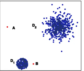
Fig. 1. An example to show the advantage of the local density estimation-based anomaly detection method over the neighborhood radius-based method.

 Local anomaly factor-based methods use the ratio of the neighborhood density of a given sample, measured using the local densities of the neighbors of the sample, to the local density of the sample to

determine the anomaly factor of the sample [7]. The less the local density of a sample and the larger its

neighborhood density, the larger the anomaly factor of the sample. The local anomaly factors for normal

samples fluctuate around 1 and the local anomaly factors for anomalies are much larger than 1. This can

distinguish anomalies from normal samples more clearly. Fig. 1 shows an example that the local anomaly

factor-based methods have advantages in contrast with the neighborhood radius-based methods. In the figure,

the blue points represent normal samples distributed in the denser cluster D1 and the less dense cluster D2.

The red points A and B represent anomaly samples which are isolated from the two clusters. Anomaly A is

neighborhood density of Anomaly B is high, it is easily detected by the local density estimation-based

method. Latecki et al. [9] proposed a typical local anomaly factor-based anomaly detection method.They

used the Gaussian kernel to estimate local densities of samples. The shape of the whole neighborhood was

adjusted using the covariance matrix of the Gaussian. The limitations of Latecki et al’s work [9] are that the

influence of the size of the neighborhood is not considered and the global properties of the distribution of

the samples are ignored. Schubert et al. [56] formulated an excellent generalization of a density-based

anomaly detection method based on kernel density estimation. They applied the z-score transformation to

standardize the deviation from normal density. The normal cumulative density function was used to

normalize the scores to the range [0, 1], and then a rescaling was applied to obtain the anomaly score.

Schubert et al.’s method [56] has flexible applicability and scalability.

 The local correlation integral-based methods [8] use the number of neighbors in a fixed radius of a sample to measure the local density of the sample. The distance between the Gaussian distributions of the

local density of a given sample and the local densities of its neighbors is used as the anomaly factor of the

sample. For a given sample, the maximum of the anomaly factors obtained using different neighborhood

radiuses is used to measure the possibility that the sample is an anomaly. These methods avoid the choice of

the neighborhood size k, but require more computational cost.

 The local peculiarity factor-based methods [10] compute the anomaly factors for each feature dimension and the weighted average of these anomaly factors for a sample is used as the final anomaly factor for the

sample. The computational complexity has a direct correlation with the number of dimensions of feature

vectors. Therefore, these methods are not adapted to high-dimensional datasets.

The local density-based methods [20] are unsupervised and can be applied to complex datasets with sparse or dense

mixed samples of different types. However, overall the current local density-based methods have the following

common limitations:

 Local density estimation is not accurate enough, which leads to a reduced performance.

 Their performance depends on the choice of the neighborhood size parameter.

 These methods are based on local analysis. The global properties of the distribution of the samples are ignored.

1.2. Our work

In this paper, we focus on local density-based anomaly detection, aiming at removing the above limitations in

local density estimation-based anomaly detection. We propose a new anomaly factor estimation method which uses

the ratio of the weighted neighborhood density to the local kernel density of a sample as the anomaly factor of the

sample and uses hierarchical context-based local regression to refine the anomaly factors of each sample. The main

 We propose a new kernel function, the Volcano kernel, which is more appropriate for estimating the local densities of samples and then detecting anomalies.

 We propose a weighted neighborhood density estimation which is more robust to the neighborhood size parameter than the traditional averaged neighborhood density estimation.

 We propose a multi-scale local kernel regression method together with a new context-based kernel function to combine the information from multiple scale neighborhoods for locally and globally refining the samples’

anomaly factors.

 We apply the proposed general anomaly detection methods to image saliency detection, based on local

density estimation of visual features and saliency score propagation in the image. Our method uniformly

highlights entire salient regions in contrast with previous methods which only produce high saliency scores

at or near object edges [49, 50].

The remainder of this paper is organized as follows: Section 2 proposes our anomaly detection method based on

local kernel and weighted neighborhood density. Section 3 presents our anomaly factor refinement method based on

the hierarchical context-based kernel regression. Section 4 applies our anomaly detection methods to image saliency

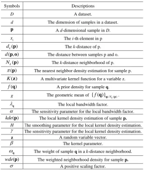
detection. Section 5 reports the experimental results. Section 6 concludes the paper. Table 1 clarifies notations in the

paper, helping keep track of symbols’ meaning.

Table 1. Symbol Table

Symbols Descriptions

D A dataset.

d The dimension of samples in a dataset.

p A d-dimensional sample in D.

i

x The i-th element in p

( )

k

d p The k-distance of p.

( , )

d p o The distance between samples p and o.

( )

k

N p The k-distance neighborhood of p.

( )

 p The nearest neighbor density estimation for sample p.

( )

K z A multivariate kernel function for a variable z.

( )

f q A prior density for sample q.

g The geometric mean of { ( )} _{( )}

k N

f q _{q p} .

q The local bandwidth factor.

 The sensitivity parameter for the local bandwidth factor.

( )

kdep The local kernel density estimation of sample p. H The smoothing parameter for the local kernel density estimation.

 _{The sensitivity parameter for the local kernel density estimation.}

z A random variable vector.

 The kernel parameter.

q The weight of sample q in a k-distance neighborhood.

( )

wdep The weighted neighborhood density for sample p.

( )

WAF p The weighted anomaly factor for a sample p.

N The number of samples in a dataset.

i

x The i-th sample in the dataset.

i

y The estimated anomaly factor for x_i.

t The iteration step index.

j

c The value vector of pixel j in the CIE L*a*b* color space. i

I The image patch centered at pixel i. i

v A feature vector describing I_i

j

 The weight for pixel j.

dspatial(i, j) The Euclidean distance between positions of pixels i and j.

( )

S i The saliency score for pixel i.

L An image multi-scale set.

2. Local Kernel Density-Based Anomaly Detection

A density estimation-based method detects anomalies by comparing the density of each sample with its

neighborhood density which is usually the average of the local densities of its neighbors [7]. We propose a new

kernel function for local density estimation and a weighted neighborhood density to calculate each sample’s anomaly

factors which are used to detect anomalies. Our anomaly detection method based on the weighted neighborhood

density is robust to the neighborhood size parameter.

2.1. Definition of neighborhood

Fig. 2. 3-distance neighborhoods.

Let D be a dataset and let D be the number of the samples in D. Let p[ ,x x_{1 2},...,x_d] be a d-dimensional sample in D. For any positive integer k (k D ), the k-distance dk( )p of p is defined as the distance d( , )p o between p and a sample oD, such that in D\{ }p

 there are at least k samples q of which holds that d( , )p q d( , )p o ,

 there are at most k-1 samples q of which holds that d( , )p q d( , )p o .

than the k-distance of p: Nk( )={p qD\{ } ( , )p d p q dk( )}p . Any sample q in Nk( )p is called a k-distance

neighbor of p. In Fig. 2, the red points are normal samples and the blue point is an anomaly. In particular, the point p2

is a normal sample and the point p1 is an anomaly. The 3-distance neighborhood of p2 is obviously less than the

3-distance neighborhood of p1, i.e., k-distance(p2)<k-distance(p1). The size of the k-distance neighborhood of a

sample in the space has an inverse relation to the local density of the sample. Given k, the denser the samples, the

smaller the k-distances of these samples.

2.2. Local kernel density estimation

The density estimation methods in common use include histogram-based, nearest neighbor-based, and

kernel-based methods [6]. The histogram-based density estimation is simple to implement and has a low time

complexity. But its distribution density is discrete (not a smooth curve) and it is seldom used for anomaly detection.

The nearest neighbor density estimation is defined as:

1 ( )

2 k( )

k D d

 p  

p . (1)

The limitations of the distribution curve yielded by the nearest neighbor density estimation are that the curve is not

smooth and the integral over it does not equal to 1 [6]. As shown in Fig. 3, the heavy tails of the density function and the discontinuities in the derivative for the nearest neighbor density estimate reduce the accuracy of the density

estimate. This reduction may lead to an increase in errors of anomaly detection for complex and large databases. By

using kernel functions, the kernel density estimate yields a smooth distribution curve over which the integral equals

1. The size of the window can be used to adjust the smoothness of the curve.

(a) Old Faithful data (b) Density estimate

Fig. 3. (a) The lengths of 107 eruptions of Old Faithful geyser; (b) The density of Old Faithful data based on the nearest neighbor density estimate, redrawn from [6].

We extend the standard kernel density estimation [6] to a type of local kernel density estimation and propose to

for a variable vector z. Let f( )q be a prior density for sample q. Let g be the geometric mean of { ( )}f q qNk( )p :





( )

log ( ) exp ( ) k N k f g = N           



p (2)

where Nk( )p is the number of the k-distance neighbors of p. Let q be the local bandwidth factor:

( ( ) / )f g 

 _ 

q q , where  is the sensitivity parameter that satisfies o  1. The local kernel density estimation of

a sample p is defined as:













( ) ( ) ( ) k N k

h K h

kde N _  _       



p (3)

where h is the smoothing parameter and  is the sensitivity parameter. We explain the following points with respect to (3):

 As in traditional kernel density estimation, the local kernel density estimation adaptively adjusts the kernel window size from one sample to another according to the value of q.

 The kde( )p is computed locally in the k-distance neighborhood of sample p, rather than in the entire dataset for the traditional kernel density estimation. Therefore, the computational complexity is greatly

reduced.

 In the traditional kernel density estimation [6], the parameter  is set to the dimension d of the sample feature vectors. For the local kernel density estimation, a large value of  may make kde( )p unstable or sensitive. For example, if _q is very small, then (_q) approximates infinity. We experimentally

determine an appropriate value of  as  2 using cross verification to maintain a balance between sensitivity and robustness.

 In kde( )p , the window adjustment parameter q depends on the prior density function f( )q . It is

required that f( )q can, overall, contrast local densities of different samples. As the k-distance of q is inversely related to the local density of q, we estimate f( )q as follows:

1 ( ) ( ) k f d  q

q . (4)

We substitute (4) into (3), and then the local kernel density of sample p becomes:

2 ( ) 1 ( ( ) ) ( ( )) ( ) ( ) k

N k k

k K

C d C d

kde N          _{ }

q



p q

q q

p

p (5)

2.3. Kernel function

The kernel function in (5) is very important for density estimation. The multivariate Gaussian function and the Epanechnikov kernel function are commonly used in the kernel density estimation. However, the Gaussian kernel

and the Epanechnikov kernel are not appropriate for use in (5). Therefore, we define a new kernel function which is

more appropriate for our kernel-based anomaly factor method to detect anomalies.

The multivariate Gaussian kernel function is defined as:

2

/ 2 1

( ) exp 2

d

K   _ _

 

z=(2 ) z (6)

where z denotes the Euclidean norm of a variable vector z. The Epanechnikov kernel function is defined as:

2

(3 / 4) (1 ), 1

( )

0,

d

if K

otherwise

 _{ }

   

z z

z . (7)

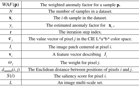
Fig. 4 shows the curves of the Gaussian kernel and the Epanechnikov kernel. The traditional local density-based

anomaly detection methods, which usually use the ratio of its neighborhood density to its local density as its anomaly

factor, have the advantage that the obtained anomaly factors of normal samples fluctuate around “1” and the obtained

anomaly factor values of anomalies are obviously larger than “1”. But, if the Gaussian kernel is used for estimating

anomaly factors, it is not guaranteed that the anomaly factors of normal samples within a cluster are approximately

equal to 1. This makes it difficult to determine the threshold value for anomaly factors. As shown in Fig. 4, the

Epanechnikov kernel function equals zero when z is larger than 1. If the Epanechnikov kernel is used for estimating anomaly factors, most of anomalies and normal samples lying in the borders of clusters have anomaly

factors equal to infinity. This influences the results of anomaly detection.

Fig. 4. The shapes of the curves of the Gaussian kernel and the Epanechnikov kernel.

In order to avoid the limitations in using the Gaussian kernel and the Epanechnikov kernel for estimating

, 1 ( )

( ),

if K

otherwise

 

 

  

z z

z

= (8)

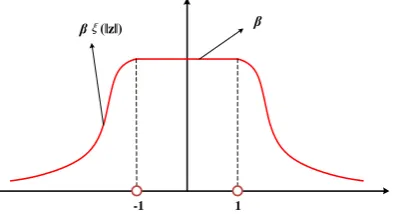
where  is chosen such that K( )z integrates to one, and (z) is a monotonically decreasing function taking values in the closed interval [0,1] and tending to zero at the infinity. We use (z)exp( z 1) as the default function. The mathematical derivation of β is included in Appendix A. Fig. 5 shows the curve of our Volcano kernel

function in a univariate feature space. When z 1, the kernel value equals a constant  . This ensures that the anomaly factors of the samples within a cluster approximate to 1. When z 1, the kernel value is less than 1 and monotonically decreases as z increases. This makes the anomaly factors of anomalies much larger than 1. Hence, the proposed kernel function is suitable for anomaly detection.

Fig. 5. The curve of the proposed Volcano kernel function in a univariate feature space.

The neighborhood size k needed by our Volcano kernel is less than the neighborhood size k needed by the

Gaussian kernel and the Epanechnikov kernel. The reason is that the Gaussian kernel and the Epanechnikov kernel

are designed to estimate the distribution densities of samples. The larger the value of k, the more samples are

involved in density estimation and the more accurate the density estimate. However, our Volcano kernel is

specifically designed to detect anomalies. Its motivation is to make the anomaly factors of normal samples

approximate to 1 and the anomaly factors of anomalies much larger than 1. The values of the random variable z

for normal samples, which are the majority of the samples in the dataset, lie between -1 and 1. For our Volcano

kernel, only a line segment is used to represent the densities when z is within [-1,1] as shown in Fig. 5, while a curve segment is used for the Gaussian kernel or the Epanechnikov kernel as shown in Fig. 4. It is apparent that

estimation of the density of a sample using the Volcano kernel requires fewer neighboring samples than estimation

using the Gaussian kernel or the Epanechnikov kernel. Therefore, our Volcano kernel requires a smaller

neighborhood size k.

2.4. Weighted neighborhood density

The performance of local density-based anomaly detection depends strongly on the choice of an appropriate

value of the neighborhood parameter k. Only when k is large enough such that most of the samples in the

neighborhood are normal, can the anomalies be detected. In order to increase the robustness to the parameter k, we

1 -1

propose a weighted neighborhood density, in contrast with the traditional neighborhood density which is the average

of the local densities of all the neighbors of a sample and is sensitive to the presence of anomalies in the

neighborhood.

The weighted neighborhood density wde( )p is defined for a sample p as follows:

( )

( )

( ) ( ) k

k N N kde wde      





p (9)

where q is the weight of sample q in the k-distance neighborhood of sample p. The weight q is inversely

related to the k-distance of q, and we define it as follows:

2 2 ( ) 1 exp 2 k k d min    _{ }   _  _   _{ }   _ _       q q (10)

where  is a positive scaling factor and

( )

min ( ( ))

k k k N min d  

q p q . (11)

The weight of a neighboring sample is a monotonically decreasing function of its k-distance. The neighboring

sample with the smallest k-distance has the largest weight which equals 1. Other neighbors’ weights lie within

interval (0,1). The k-distance of a sample describes its local density: The more the k-distance, the less the local

density. It follows that the weight of a neighboring sample depends on the density of this sample. For a normal

sample, its neighboring samples are mostly normal, and its weighted neighborhood density is similar to its average

neighborhood density. But for an anomaly, the proportion of anomalies in its neighborhood is uncertain when the

parameter k is small. When a large proportion of samples are anomalies in the neighborhood of an anomaly, the

average neighborhood density may be drastically decreased, which influences the detection of the anomaly. However,

the weighted neighborhood density of an anomaly is obviously larger than the average neighborhood density.Then,

the anomaly is easier to detect using the weighted neighborhood density. Therefore, the range of appropriate values

of k for the weighted neighborhood density estimation is much wider than the range for the traditional average

neighborhood density estimation. This means that our weighted neighborhood density estimation is more robust to the

variations in the value of k. Our weighted neighborhood density estimation can replace the average neighborhood

density estimation in any local density-based anomaly detection method, and make the method less sensitive to the

parameter k.

2.5. Anomaly factor estimation

The anomaly factor is used to estimate the extent to which a sample is an anomaly. Normal samples lie in dense

and have low local densities. The local kernel density and weighted neighborhood density-based anomaly factor

( )

WAF p of a sample p is defined as:

( ) ( )

( )

wde WAF

kde

 p

p

p (12)

The less a sample’s local kernel density and the larger the weighted density of its neighborhood, the larger the

anomaly factor and the more probably the sample is an anomaly. For most anomalies which are isolated from the

cluster, their local densities are much different from their neighborhood densities, ensuring that their anomaly factors

are much larger than 1. For most samples in a cluster, their local densities are closer to their neighborhood densities,

ensuring that their anomaly factors fluctuate around 1. This makes it easy to distinguish between anomalies and

normal samples.

Given the anomaly factors of all the samples, the anomalies are detected in the following ways:

 The top N samples listed in the descending order of anomaly factors are considered as anomalies.

 The samples whose anomaly factors are larger than a threshold are considered as anomalies.

Appendix B gives a mathematical proof of the claim that the weighted neighborhood density estimation is more

robust to the parameter k than the traditional average neighborhood density estimation for anomaly factor estimation.

This gives a theoretical support to the robustness of our anomaly detection method to the neighborhood size

parameter.

2.6. Computational complexity

Computation of the anomaly factors based on local kernel density and weighted neighborhood density includes

the following two steps:

 The k-distance neighbors for each sample are found.

 The whole dataset is traversed, and the kde( )p , wde( )p , and WAF( )p values for each sample p are computed.

Without optimization, the computational complexity of the first step is 2 ( )

O n where n is the number of samples in the dataset. By optimization using an index technology, such as the K-D index tree algorithm [7, 20], the

computational complexity is reduced to O n( log )n . The computational complexity of the second step is O nk( ), since both kde( )p and wde( )p are computed in the k-distance neighborhood of p. Hence, the total computational complexity of our local kernel and weighted neighborhood density-based anomaly detection method is

( )

O n log n+ nk . The larger the k _{is, the more the runtime. Increasing the robustness to the parameter} k not only

overcomes the difficulty in determining the value of k without any prior knowledge, but also ensures that a lower

2.7. Limitations

There are the following two limitations in the local kernel density-based local anomaly factor estimation

method:

 Anomaly factors are not accurate enough to rank all the samples in the database. In the local density-based methods, the anomaly factor of a sample is determined by both the estimate of its density and the density

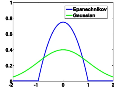
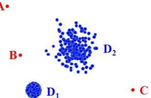
estimate of its neighborhood. As shown in Fig. 6, sample A is close to cluster D2 and sample B is close to

cluster D1. Cluster D1 has a larger density than cluster D2. Then, the estimated anomaly factor of sample A

is smaller than that of sample B. However, as sample A is farther away from the normal sample clusters, it

has a higher probability of being an anomaly than sample B in practice.

 The local kernel-based local anomaly factor of a sample depends on the density estimation in its neighborhood. The estimated local anomaly factors in the same cluster may differ widely because of

different neighborhood densities. With a fixed value of k for all the samples, the neighborhood density

estimation may not be accurate enough to express the relative magnitudes of the neighborhood densities of

different samples. If the anomalies are randomly distributed in a number of clusters that have different

densities, a single value of k may not be appropriate for detecting all the anomalies. Then, the estimated

local anomaly factor values are not accurate enough to rank all the samples in a complex database with

highly variable region densities.

Fig. 6. The inaccurate anomaly factors for local density-based methods.

3. Hierarchical Context-Based Kernel Regression

In order to handle the above limitations of local density-based methods, we propose to adopt non-parametric

regression to refine the anomaly factors obtained by a local density-based method F(). The dataset { ,x x1 2,...,xn}

is preprocessed:

( )

1 1 1

{ ,..., } {( , ),..., ( , )}

F

n  y yn n

x

x x x x (13)

where y_i is sample x_i’s anomaly factor estimated by F( )x . We propose a multi-scale local kernel regression method to combine the information from multiple scale neighborhoods to hierarchically refine the anomaly factors

1 2

3.1. Local kernel regression

Nadaraya-Watson kernel regression is a classic nonparametric regression method [21]. It has strong adaptability,

high robustness, and unfettered regression function forms. It is able to effectively handle nonlinear inhomogeneous

regression problems.

Given a dataset {( ,y₁ x₁), (y₂,x₂),..., (y_n,x_n)}, the Nadaraya-Watson kernel regression estimates the dependent parameter y of a vector x in the following way:

1 1 1 ( ) 1 ( ) n i i

i i i

n

i

i i i

K y y K                       





x x (14)

where _i is an adaptive smoothing parameter,  is a sensitivity parameter, and K() is a multivariate kernel function. The Nadaraya-Watson kernel regression attains the estimation of y for sample x using the weighted average of { ,...,y₁ y_n}. The weight depends on:

 the kernel function K() which determines the mapping relation between the weight of x_i and the difference between x and x_i.

 the parameter _i which determines the size of the window of the kernel function.

Intuitively, the less the difference between x and xi, the larger the weight for xi, and the closer the value y is to yi.

The Nadaraya-Watson kernel regression estimator avoids the parameter solving process in the traditional linear

regression models. It is more adaptable to complex samples which are nonlinearly distributed. The limitation of the

Nadaraya-Watson regression is that it is necessary to traverse all the samples in the dataset to estimate the regression value of a new sample, and then the computational complexity is high.

To reduce the computational complexity of the Nadaraya-Watson regression, we extend it to propose a local

kernel regression estimator which is computed locally in the k-distance neighborhood of a sample. The local kernel

regression estimator of a sample p is defined as:









N k k

N _k k

K y d d y K d d                   





where sample q is a k-distance neighbor of p and y_q is the anomaly factor of q. The local kernel regression estimator is different from the Nadaraya-Watson kernel regression in the following ways:

 The computational complexity of the Nadaraya-Watson regression for estimating the dependent parameter of a sample is O(n). The computational complexity of our local regression estimator for a sample is O(k). It

Nadaraya-Watson regression estimator.

 In the Nadaraya-Watson regression, the parameter  is usually set to the dimension d of the sample vectors. In high dimensional databases, (k-distance)d is unstable, because when k-distance is small (k-distance)d

approximates to 0, and when k-distance is large (k-distance)d is very large. This makes the regression

estimator indiscriminative to samples. To obtain a balance between the sensitivity and the robustness, a

default value of  is 2, which is verified as an optimal value by our experiments.

 The window control parameter _i for a sample i in the Nadaraya-Watson regression becomes the

k-distance of the sample in our local kernel regression estimator. We use the k distance of each sample in the

neighborhood to control the size of the window. This ensures that the size of the window is adaptively

adjusted in a data-driven way. Selection of the parameter  for a sample as in the Nadaraya-Watson regression is avoided.

3.2. Context-based kernel

The kernel K() in (15) is critical for determining the performance of the local kernel regression. The kernel

function in the local regression has the following requirements:

 It should effectively keep high anomaly factors for the isolated anomalies which can be easily detected by the local anomaly detection methods, such as our method based on local kernel and weighted neighborhood

density.

 It should make the anomaly factors of anomalies in the same cluster close to each other and obviously distinguishable from the factors of normal samples.

The local kernel function should be able to utilize the relation between a sample and its k-distance neighbors, besides

only using the differences between samples and the neighborhood size to determine the weight of each neighbor.

The traditional kernels, such as the Gaussian kernel and the Epanechnikov kernel, cannot meet the above

requirements. So, we propose a new kernel function which is defined as follows for a variablevector z:





, 1

( ) 1

exp ,

2

if K

otherwise





 

 _{ }

 _  _



 _{ }

 _{ }



z

z z (16)

where the constant  is chosen to ensure that K() integrates to 1(The mathematical derivation of β is included

in Appendix A). Based on the new kernel, the local kernel regression estimator computes the weight of a k-distance

neighbor q of a sample p according to the followed rules:

 If p is also a k-distance neighbor of q, then p q d_k( )q and

( )

K

d 

  _    

p q

 If p is not a k-distance neighbor of q, then p q dk( )q , and

2

1 ( ) )

exp

( ) 2

k

k

d K

d 

 _{  }         _ _  

   

   

 

 

p q q p q

q . (18)

The kernel value of q is, with the maximum β, a monotonically decreasing function of the difference between p and q.

The reason for the first rule is that, if either of two samples is a neighbor of the other sample, then they have similar

local distributions and they are likely to belong to the same cluster. Therefore, both of them are assigned larger

weights to obtain similar anomaly factors. The reason for the second rule is that, if only one of two samples is a

neighbor of the other sample, then they are less closely related, and thus we use their difference to inversely weight

them. In this way, our neighborhood context-based kernel retains the properties of the traditional kernels. It also

considers the different properties of isolated anomalies and anomalies distributed in clusters and deals with these two

types of anomalies differently. By combining similarities between samples and the neighborhood context, our kernel

can more effectively distinguish anomalies from normal samples.

3.3. Hierarchical kernel regression

A complex dataset includes anomalies which are easier to detect by taking into account the global distribution

of all the samples and anomalies which are distributed in small clusters and are easier to detect locally. We propose a

hierarchical kernel regression strategy which iteratively updates anomaly factors of samples using our local kernel

regression method by gradually enlarging the size of the neighborhood. In this way, sample anomaly factors are

estimated both locally and globally to increase their accuracies.

The hierarchical kernel regression-based anomaly detection method initializes the anomaly factors 0 0 1 {y ,...,y_n}

for the samples using the anomaly factors obtained by the local kernel density and weighted neighborhood

density-based method described in Section 2. The initial value k₀ of k for the hierarchical updating process is set to

the value of k used in the initial anomaly factor estimation. Isolated anomalies should be specifically handled to

avoid that the anomaly factor of an isolated anomaly is smoothed by its k-neighbors. As shown in Fig. 6, isolated

samples are obviously far from other samples. We propose to use the neighborhood context to identify isolated

anomalies, i.e., if a sample is not a k-neighbor of its own k-neighbors, then there is no similar sample in its

neighborhood and the sample is treated as an isolated sample. The anomaly factors of isolated anomalies are kept

unchanged, because the anomaly factors of the isolated anomalies usually have been accurately estimated by the

initial local density-based method.In this way, our regression method effectively handles the isolated anomalies and

increases the accuracy of detecting anomalies distributed in clusters. Our hierarchical kernel regression-based

Step 1: 1t; k₀k; 0 0 1

{y ,...,y_n} is given.

Step 2: Determine the k-distance neighborhoods for all the samples.

Step 3: Compute { ,...,y₁t yt_n} using the local kernel regression estimator (15), given 1 1 1

{yt ,...,ynt }

  _;

If  q Nk( )p p q dk( )q , then p is identified as an isolated anomaly and

1

t t

y_py_p .

Step 4: If 1

1| |

n _{t t}

i i

i y y



 



Step 5; otherwise t 1 t, k  k( is a stepping factor), and go to Step 2 for another loop of iteration.

Step 5: Output the anomaly factors { ,...,₁t t}

n

y y .

Our hierarchical kernel regression combines the multiple scale information from the different sizes of

neighborhoods using the local kernel regression estimator. This combination makes the hierarchical kernel regression

more effective in detecting anomalies in mixed and large databases.

4. Spatial Constrained Anomaly Detection: Image Saliency Detection

We apply the above general anomaly detection theory to image saliency detection [47, 48], and propose a

spatial constrained anomaly detection method. Salient regions in an image deviate from the background regions and

capture the attention of human viewers. This makes it possible to treat salient pixels in object regions as anomalies

and background regions as normal, and then use our unsupervised anomaly detection method to construct a saliency

map. In contrast to pure anomaly detection, saliency detection combines visual feature contrast information and

pixels’ spatial distribution information. A saliency detection method is proposed, which consists of local

density-based saliency map computation in the feature space and saliency score propagation in the image.

4.1. Local density-based saliency map

According to the human vision attention mechanism theory, the saliency of a pixel depends on its appearance

and its context with its surrounding pixels. Hence, we use visual features of the image patch centered at each pixel,

instead of only the pixel value itself. Let c_j be the value vector of pixel j in the CIE L*a*b* color space. A pixel i

is represented by a visual feature vector v_i describing the image patch I_i centered at pixel i:

i i j j j I i j j I     





v (19)

where _j is the weight for pixel j. The weight is computed by:

2 ( , ) 1 exp 2 2 spatial j

d i j

 

 

 _ _

  (20)

the appearance of its patch I_i deviates from the majority of patches in the visual feature space. Given the visual

feature vector set { }v_i of all the patches in an image, we propose to estimate the saliency score S i( ) for each pixel i using anomaly factor obtained by comparing the local density of the patch I_i with its neighborhood density

using the anomaly detection method in Section 2.

We use local density estimations from multi-scales which are obtained by shrinking (subsampling) the original

image, to improve the saliency scores. As a prior knowledge, background patches always have more similar

appearances than salient patches. This indicates that a background patch and its k-nearest neighbors in the visual

feature space follow the more similar distributions than a salient patch in multi-scales. For each shrunken image, we

estimate its saliency map and then enlarge the saliency map to the same size as the original image. In this way, a

number of saliency scores for each pixel in multiple scales are obtained. To improve the visual contrast between

salient patches and background patches, we combine these saliency scores by:

1

( ) l( )

l L

S i S i L 





where S i_l( ) is the saliency score of pixel i in a scale l, and L is the multi-scale set with the size of L .

4.2. Kernel-based saliency score propagation

The above local density-based saliency map computation captures the salient pixels which are the foci of human

attention. We keep the original saliency scores of the pixels which have large saliency scores, and propose a

kernel-based saliency score propagation method to adjust the saliency scores of other pixels. This propagation

method which is similar to the local kernel regression in Section 3.1 is defined as follows:

{ ( ), } { ( ), } ( ) ( ) ( ) ( ) k Spatical k Spatical i j

j N i i k j

i j

j N i i k j

K S j d S i K d                     





where K() is a kernel function as defined in (16), and different from (15) the neighborhood N_Spatialk ( )i is defined in

the image space rather than in the visual feature space. Our kernel-based saliency score propagation method causes

that pixels in the same salient region achieve closer saliency scores. According to the definition of K(), if either of

patch i and one of its spatial neighbors lies in the k-nearest neighborhood of the other patch in the feature space, the

weight of the spatial neighbor patch is set to be the maximum. Our saliency score propagation method ensures that

pixels spatially near to the pixels which have large saliency scores increase their saliency scores, while the background pixels have low saliency scores.

5. Experiments

methods on several synthetic and real datasets. We compared our image saliency detection method with the

state-of-the-art methods on a publicly available dataset. In the experiments, there are a few parameters and

thresholds which were determined by cross-validation. The parameter  in (3) was set to 2. The parameters 

and C in (5) were set to 1. The parameter  in (10) was set to 1 except for testing the effect of  . The parameter

 in (15) was set to 2. The initial value k0 of k for the hierarchical context-based kernel regression updating

process was set to 1.5% of the number of samples in the dataset. The stepping factor  was set to 2.5% of the number of samples in the dataset. The maximum number of iterations was set to 5. For image saliency detection,

each pixel was expressed by a patch of size of 7*7 pixels. Saliency scores in (21) were computed in the four scales

which correspond to the sizes of 100%, 50%, 25%, and 12.5% of the original image. The neighborhood size in the

image space in (22) was set to 10% of the number of pixels in the image.

In the following, we first evaluated the robustness of our local kernel and weighted neighborhood density-based

method to the neighborhood parameter k on two synthetic datasets. Then, we compared our local kernel and

weighted neighborhood density-based anomaly detection method and the hierarchical local regression-based method

with several state-of-the-art anomaly detection methods on several real datasets. Finally, the comparison results for

image saliency detection were reported.

5.1. Synthetic datasets

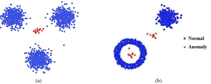
Fig. 7 shows two synthetic datasets. The Synthetic-1 dataset consists of 1500 normal samples and 16 anomalies.

The normal samples are distributed in three clusters where each cluster contains 500 normal samples. Fifteen

anomalies lie in a cluster whose center is equidistant from the centers of the three clusters of the normal samples; and

one anomaly is isolated from all the others. The Synthetic-2 dataset consists of 1000 normal samples and 20

anomalies. There are 500 normal samples uniformly distributed in an annular region and 500 normal samples

distributed in a cluster. There are 10 anomalies lying in the center of the annular region and 10 anomalies distributed

between the two clusters of the normal samples.

(a) (b)

Fig. 7. The distributions of two synthetic datasets: (a) Synthetic dataset 1; (b) Synthetic dataset 2.

work. In the baseline [7], the local anomaly factor of a sample is the ratio of its neighborhood density to its own

density. Table 2 shows the anomaly detection results of the baseline [7] and our method on the Synthetic-1 dataset,

when the weight parameter  in (10) was set to 0.1 and 1. The performance of anomaly detection was estimated using the number and proportion of the anomalies in the 16 samples which have the largest estimated anomaly

factors. It is seen that our local kernel and weighted neighborhood density-based method identifies all the anomalies

when k27 and σ = 0.1 and detects all the anomalies when k31 and σ = 1. The baseline is unable to identify all the anomalies until k60. This indicates the following points:

 The available range of k _{for our method is much larger than the range for the baseline. So, our method is less}

sensitive to the parameterk.

 The value of k for our method to reach the best performance is much smaller than that for the baseline, so our method can obtain the same result as the baseline with less runtime.

 Our method is robust to the parameter  .

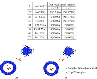
Table 2. Results of anomaly detection on the Synthetic-1 dataset: the number and proportion of anomalies in the top-16 samples

k Baseline [7] Our local kernel method σ = 0.1 σ = 1 26 1(6.25%) 15(93.75%) 15(93.75%) 27 2(12.5%) 16(100%) 15(93.75%) 30 4(25%) 16(100%) 15(93.75%) 31 5(31.25%) 16(100%) 16(100%) 59 15(93.75%) 16(100%) 16(100%) 60 16(100%) 16(100%) 16(100%) 70 16(100%) 16(100%) 16(100%)

(a) (b)

Fig. 8. The best results of our method and the baseline on the Synthetic-2 dataset: (a) The results of our local kernel and the weighted neighborhood density-based method with k=14; (b) The results of the baseline [7] with k=20.

Fig. 8 shows the best results that our method and the baseline obtain on the Synthetic-2 dataset. It seen that our

method captures all the anomalies in the top-20 sample list of anomaly factors when k=14. The baseline obtains its

best performance when k=20, and only 17 anomalies are correctly detected in its top-20 sample list. Compared with

our method, the baseline cannot detect all the anomalies whatever the value of k, because the annular cluster

our method is more adaptable to the complex datasets than the baseline.

5.2. Real datasets

The following public real datasets were used to compare our methods with the state-of-the-art anomaly

detection methods:

 The KDD Cup 1999: This is a general dataset for network intrusion detection research. The 60593 normal sample and the 228 U2R attack samples labeled as anomalies were selected to form the KDD dataset for

anomaly detection. Each sample is described by 41 features.

 The Mammography dataset: This dataset was extracted from a mammography image dataset. It includes 10923 normal samples and 260 anomalies. Each sample consists of 6 features.

 The Ann-thyroid dataset: This is a dataset of pathological thyroid changes. It consists of 73 anomalies and 3178 normal samples. Each sample consists of 21 features.

 The Shuttle dataset: This dataset has six classes in which there are 11478, 13, 39, 809, 4, and 2 samples, respectively. Five test datasets were constructed. The samples in the largest class become the normal

samples in all the five test datasets. The samples in one of the other five classes become anomalies in a test

dataset. Each sample is described by a 9-dimensional feature vector.

 The visual trajectory dataset: The trajectories in this dataset were captured by tracking vehicles in a crowded traffic scene. There are 1500 normal trajectories and 50 anomalies which correspond to traffic

offences or tracking errors. Each trajectory was linearly interpolated with points to ensure that all the

trajectories have the same number of points. The coordinates of the points in a trajectory form a vector

representing the trajectory.

The samples in these datasets were preprocessed by the inverse document frequency method [10, 13, 14] in order

that the discrete features can be handled in the same way as the continuous features.

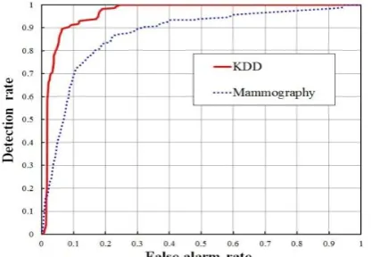
Fig. 9. ROC curves of our local kernel and weighted neighborhood density-based method on the KDD and the Mammography datasets.

the y-coordinate and the false alarm rate as the x-coordinate. As an example, Fig. 9 shows the ROC curves of our

local kernel and weighted neighborhood density-based method on the KDD dataset and the Mammography dataset.

The AUC value is the surface area under the ROC curve. The larger the AUC value, the more accurate the anomaly

detection result. The AUC value on the Shuttle dataset is the average AUC of all the five subsets.

Table 3. The AUC values of our local kernel and weighted neighborhood density-based method with different kernels on the real datasets

Datasets

Kernels KDD Mammography Ann-thyroid Shuttle (average) Trajectory

Our kernel 0.962 0.871 0.970 0.990 0.979

Gaussian kernel 0.961 0.870 0.970 0.990 0.976

Epanechnikov kernel 0.944 0.855 0.965 0.993 0.973

Table 4. The runtimes (seconds) of our local kernel and weighted neighborhood density-based method with different kernels on the real datasets

Datasets

Kernels KDD Mammography Ann-thyroid Shuttle (average) Trajectory

Our kernel 1918.1 15.8 4.9 36.4 4.1

Gaussian kernel 2095.2 19.8 5.2 36.9 5.5

Epanechnikov kernel 2363.7 48.2 13.2 66.7 12.3

Fig. 10. Thevalues of k with the best results for different kernels.

We compared the performances of our local kernel and weighted neighborhood density-based method when the

Gaussian kernel, the Epanechnikov kernel, and our Volcano kernel were used respectively, where the parameters and

thresholds were kept unchanged. Tables 3 and 4 show, respectively, the AUC values and the runtimes of our local

kernel and weighted neighborhood density-based method with different kernels on the real datasets. Fig. 10 shows

the values of k for all the three kernels on all the datasets when the best detection results were obtained. It is seen that

although the detection accuracy of our Volcano kernel is overall only slightly higher that the detection accuracy of

the Gaussian kernel and the Epanechnikov kernel, the neighborhood size k with the best results for our Volcano

kernel are smaller than those of the other kernels.This supports the claim that our kernel achieves the least runtime.

of a normal sample using the Volcano kernel requires fewer neighboring samples than estimation using the Gaussian

kernel or the Epanechnikov kernel (See Section 2.3).

We compared our method with the following eight state-of-the-art anomaly detection methods:

 The local anomaly factor-based method [7] (the baseline of our work): The local outlier factor captures the relative degree to which the sample is isolated from its surrounding neighborhood.

 The local density factor-based method [9]: This method modifies a nonparametric density estimate with a variable kernel to yield local density estimation. Anomalies are then detected by comparing the local

density of each sample to the local density of its neighbors.

 The local peculiarity factor-based method in [10]: This method applies the local peculiarity factor which is the µ-sensitive peculiarity description for general distributions to anomaly detection.

 The feature bagging-based method [13]: This method combines anomaly scores computed by the individual anomaly detection algorithms that are applied using different sets of features to more accurately

detect anomalies.

 The active learning-based method [14]: This method detects anomalies by classifying a labeled data set containing artificially generated anomalies. Then, a selective sampling mechanism based on active learning

was invoked for the reduced classification problem.

 The bagging-based method in [14, 15]: The bagging method in [15] was applied to detect anomalies using the same component algorithm in [14] on the same reduced problem in [14].

 The boosting-based method in [14, 16]: The boosting-based method was applied to detect anomalies using the same component algorithm in [14] on the same reduced problem in [14].

 The generalized density-based anomaly detection method in [56]: This method produces a series of density estimates. The z-score transformation was applied to standardize the deviation from normal density. A

rescaling was applied to obtain the anomaly score.

Table 5 shows the AUC values of our method and the competing methods on the real datasets. The AUC values

of the competing methods, except for the generalized density-based anomaly detection method [56], on the KDD,

Mammography, Ann-thyroid, and Shuttle datasets were directly taken from the publications [7, 9, 10, 13, 14, 15, 16].

The setting of the parameters in these competing methods can be found in the publications. For the generalized

density-based anomaly detection method, the setting of the minimum and maximum values of k is the same as for

our hierarchical context-based kernel regression method. Other parameters were tuned to make the results as

accurate as possible. Table 6 shows the runtimes of the local density-based methods. Since the local peculiarity

factor-based method has the much higher complexity and needs much more runtime than other methods, its accurate

runtime was not given. The runtimes for the other competing methods are not available in the literature. Fig. 11