Performance analysis of a Poisson-Pareto queue over the full range of system parameters

Performance Analysis of a Poisson-Pareto Queue over

the Full Range of System Parameters

Ronald G. Addie

, Timothy D. Neame

and Moshe Zukerman

Australia, Tel +61 7 46 31 5520, Fax: +61 76 46 31 5550.

2. ARC Special Research Centre for Ultra-Broadband Information Networks (CUBIN), The University of Melbourne, Parkville, Victoria 3010, Australia.

3. Electronic Engineering Department, City University of Hong Kong, Hong Kong.

Abstract

There have been many queuing analyses for a single server queue fed by an M/G/∞ traf-fic process, in which G is a Pareto Distribution, that focus on certain limiting conditions. In this paper we enhance the so-called Quasi-Stationary (QS) approximation – a queuing analysis introduced previously that provides an algorithm for computation of an accurate approximation for the stationary queue distribution, applicable to the entire range of system parameters. By numerical evaluation of the QS approximation and the asymptotic approx-imations (large buffer, many sources, and heavy traffic) over an extremely wide range of parameter values we are able to graphically display consistency of the QS approximation with all the asymptotic results. We demonstrate that the accuracy of the asymptotic approx-imations is satisfactory only in limited regions of the system parameter space.

Key words: Large Deviation Theory, Long Range Dependence, Queueing Theory, Pareto

Distribution, PPBP

1 Introduction

The discovery that Internet traffic has Long Range Dependent (LRD) characteristics [1] has resulted in much attention given to analyses of queues with LRD input [2–28]. A popular family of traffic models that exhibits the LRD phenomenon and also captures the behaviour of Internet traffic is the one based on a Poisson arrival stream of random, heavy-tailed, or more specifically Pareto distributed bursts [2, 3, 10, 14–16, 18, 19, 22, 25, 26, 28]. This model is widely referred to as the M/G/∞traffic process. Robertset al.[29] use the namePoisson burst processfor it. The traffic model we consider is a special case of the M/G/∞traffic process in which G is a Pareto distribution. Accordingly, and following [2, 30], we call it thePoisson Pareto Burst Process (PPBP).

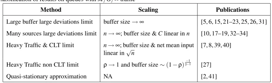
Table 1

Classification of results on queues withM/G/∞traffic

Method Scaling Publications

Large buffer large deviations limit buffer size→∞ [5, 6, 15, 21–23, 25, 26, 31] Many sources large deviations limit n→∞; buffer size &Clinear inn [10, 17–19, 32–34] Heavy Traffic & CLT limit n→∞; buffer size & net mean input

linear in√n

[7, 8, 39, 40]

Heavy Traffic non CLT limit ρ→1 and buffer size∼(1−ρ)

−1

γ−1 [27]

Quasi-stationary approximation NA [2, 41]

process. Let ρ be the ratio of the total arrival rate [bits/sec] of all active bursts to the service rate [bits/sec] of the server.

The papers [5, 6, 15, 21–23, 25, 26, 31] consider asymptotic regimes where the buffer size, or buffer threshold (in an infinite buffer case), tends to infinity while the number of sources and the server rate

C (and consequently the offered load) are fixed. This asymptotic regime is widely referred to as the

Large Buffer Limit. The papers [10, 17–19, 32–34] consider the case where the buffer size and server speed are linear in the number of sources, which tends to infinity. This is generally known as theMany Sources Limit. In both these asymptotic regimes the probability of overflow tends to zero, as either the buffer level increases or the number of sources increases, and therefore these situations are referred to asLarge Deviationslimits.

Another important case which has received attention is where the buffer size grows in proportion to √n, where n is the number of sources. This has been proposed as a practical way to provision buffers to cope with growth in traffic [35] and similar or related comments are made in [36–38]. In this literature it is assumed that the server rate also increases with the number of sources,n, in such a way that queueing performance tends to a limit not depending onn. In order that the limit of the buffer distribution exists, in these models, the server rate increases in such a way that the net mean input rate (i.e. the difference between rate of arrival of work and the server speed) also increases linearly with √

n. As n increases, the utilization tends to 1, and consequently these results are also termed, here and elsewhere,heavy traffic approximations. This literature often relies explicitly on convergence of the input traffic process to a Gaussian process, and hence we associate these results with the Central Limit Theorem (CLT). In these cases the server rate increases along with the burst arrival intensity in such a way that the CLT applies.

A different heavy traffic limit is provided in [27] where the server speed remains constant as the intensity of burst arrivals increases and the buffer level is scaled to ensure that a limit occurs. As a consequence asymptotically power-law behaviour is exhibited, much as in the large buffer large deviations results. Because in this asymptotical regime system utilization is increased towards 1, with server speed held constant, the limit is consistent with the large buffer limit in the special case where one more than the average number of flows is sufficient to overload the server. This paper also makes use of a light traffic approximation, which provides an estimate of the probability of queue non-emptiness which is asymptotically accurate as traffic becomes lighter.

than that of the tail obtained by Large Deviations Theory, suggesting that LRD queues might also have the feature that the tail behaviour of their queue distributions is not characteristic of the distribution as a whole.

In addition to these asymptotic approximations, the Quasi-Stationary (QS) approximation for the buffer level stationary distribution was presented in [2], which we here show to be a lower bound. This approximation was validated against a specially tailored type of simulation in [2]. Simulation has only rarely been used in studies of PPBP queueing systems, possibly because conventional simu-lations cannot successfully include details at the wide range of time scales needed to provide accuracy. In this paper we explore the boundaries between the regions where one or the other asymptotic ap-proximation is more accurate. The QS apap-proximation is consistent with all the asymptotic results, although the buffer level at which the large buffer approximation becomes approximately the same as the QS approximation may be, depending on the parameters of the system, rather large. All the approaches considered in this paper are summarized in Table 1.

The remainder of the paper is organised as follows. In the next section, we describe the model of a single server queue fed by PPBP input. In Section 3, we review the asymptotic results available in the literature for this system: the large buffer asymptote (where buffers increase but traffic levels stay constant), the many sources asymptote (in which buffer sizes increase in proportion to traffic), the heavy traffic approximation in which buffers increase with the square root of traffic, and the heavy traffic approximation ([27]), in which the server speed remains fixed as utilization approaches 1 and convergence to a limit occurs by scaling buffer levels. In Section 4 the QS approximation of [2], which relies on separation of traffic into long and short bursts, is further developed. A more rigorous derivation, including a demonstration that it provides a lower bound, is provided and some numerical refinements are introduced which enable the method to be used to evaluate very small probabilities, in order to be able compare the QS approximation to the large buffer asymptote in the remote regions where the two approach each other.

In Section 5, two arguments are used to show that the power-law behaviour (∼c_λxκ_{, wherex is}

buffer level) of the stationary queue distribution in a PPBP single server queue is only exhibited for a very remote region in the parameter space. First, it is shown that any power-law upper or lower bounds on the tail of the stationary complementary distribution function (CDF), or an exact asymp-totic power-law approximation for the queue stationary CDF, necessarily diverges unboundedly from the stationary queue CDF as the rate of the PPBP increases. Secondly, it is shown that the level,x_λ, where power-law behaviour begins, is unbounded as a function ofλ, the arrival rate of bursts, as it varies even over a finite range, let alone asλ−→∞.

2 The queueing model

We consider a single server queue with constant service rate,C [bits/sec], and PPBP input. As discussed, the PPBP traffic model is made up of bursts. The arrival times of each burst form a Poisson process with rateλ[bursts/sec]. Letd[seconds] be a random variable representing the burst duration. We assume that the rate at which data is generatedduringeach burst is constant for the duration of each burst and the same for all bursts, hereafter denoted byr[bits/sec]. This assumption is common in the literature, with the exception of [15, 25].

Throughout this paper, we focus on the PPBP case wheredfollows a Pareto distribution. The CDF of the Pareto distribution used in this paper takes the form:

Pr(d>x) =

(

x

δ

−γ

, x≥δ,

1, otherwise, (1)

in whichδ>0 [seconds] and γ>0. As mentioned in the Introduction,δis the scale parameter and γ is the shape parameter of the Pareto distribution. We haveE(d) =∞for 0<γ≤1, and forγ>1,

E(d) = ₍δγ

γ−1). For 0< γ< 2, the variance of d is infinite. The lower the value of γ, the heavier

the tail of the Pareto distribution becomes. In the sequel we shall generally assume that 1<γ<2 unless otherwise indicated. Thus, the PPBP queueing systems considered here are characterized by five parameters:λ,r,δ,γ, andC. In several places in the sequel we will consider a scaling in which the mean and second order statistics of the the input process minus the service process, which is termed thenet input process, will be held constant. The mean of this process shall be termed the net mean input.

An alternative definition of the Pareto distribution, in which the density is non-zero for all x∈ (0,∞), could be used without significantly affecting the conclusions of this paper. The definition (1) has the practical feature that there is a non-zero shortest burst length.

LetY_t be the amount of work [bits] that arrives between time 0 and timet, multiplied by (-1) if

t<0. Then for any real numberss, t, witht >s, positive or negative,Y_t−Y_s is the amount of work arriving between timesand timet. LetQt be the queue size process, which is also the virtual waiting time in our case where work arrives and is served continuously. By Reich’s formulaQ_t is given by

Q_t=sup s≤t

{Y_t−Y_s−C(t−s)}.

If at timet, we have thatQt>0, thebusy periodthat includes timet, is said to start at the timessuch that the above supremum occurs for this particular value ofs. By the above definitions,Y_tis stationary, thereforeQ_tis stationary, so henceforth we omit the indext, and use the random variableQto denote the stationary queue size.

The termsqueueandbufferare treated as synonymous, and we shall refer to thequeue distribution, and sometimes Complementary Distribution Function (CDF) of a queue, to mean the same thing as the distribution, or CDF, of buffer level. In an equation such asP(Q>x) =y, we shall refer toQas the stationary buffer level or queue size andxas the threshold thatQexceeds.

of our analysis are accompanied by technically precise description and no blurring of the distinction between loss and overflow is employed in any derivations. With the exception of the discussion in subsection 3.1, we concentrate onOverflow Probability P(Q>x)rather than loss probability,P_loss(x), as our key performance indicator.

3 Review of asymptotic results

Here we review existing performance analyses of Poisson-Pareto queues in four asymptotic regimes: (i) as buffer thresholds become larger and larger, with traffic and server rate fixed; (ii) as the number of sources becomes larger and larger, with the buffer thresholds and server speed increasing in pro-portion; (iii) as the number of sources becomes larger and larger, with buffer thresholds increasing in size in proportion to the square root of the number of sources; and (iv) as the number of sources be-comes larger and larger, approaching the level where the server is fully occupied, while server speed remains fixed but buffer thresholds are scaled. The first two of these asymptotic regimes apply with the considered probabilities approaching zero, and Large Deviations theory therefore supplies an ef-fective analysis method. The third of the asymptotic approximations applies to systems with overflow probabilities tending to a finite positive limit other than zero and so Large Deviations theory is not applicable. The CLT applies in this case. This case has also been described as a heavy traffic approxi-mation in [7,8], which name is justified by the fact that asλincreases, and the other system parameters are adjusted so that the probability of buffer overflow converges to a constant, systemutilizationtends to 1. The last case is a more traditional heavy traffic approximation in which the overflow probability for a fixed buffer threshold approaches 1, but by introducing a scaling of buffer thresholds the shape of the probability distribution of the overflow probability is determined for heavy traffic.

3.1 The large buffer estimate

Upper and lower power-law bounds for the loss probability,P_loss(x), in a single server queue with PPBP input process were obtained in [26]. The decay coefficient of the tail is shown to be identical for both upper and lower bounds. Large Deviations Theory was used in [22] to obtain a consistent result for overflow probabilities. Related results have been obtained in [15, 18].

The upper bound for the loss probability from [26] is

P_loss(x)≤

a(λ,C)

λγδγ(γ−1)−γ C_r +2γ−1rγ−1

k

x(−γ+1)k

λE(d)k! (2)

where

a(λ,C) =e2λ+e(λE(d)−λ)[λE(d)−λ]

C+1

(1+C)! . (3)

The lower bound from [26] is

P_loss(x)≥ γ

k_δγk_r(γ−1)k_x(−γ+1)k

λrE(d)γ(γ−1)k E(d) + (1−e−ρ∗/E(d))−1−1γ+k

whereE(d)is the mean burst duration. The parameterkis given byk=1+C_r −λE(d). Finally, the value ofρ∗ depends uponλE(d). IfλE(d)≤1 thenρ∗=λE(d), otherwise,ρ∗may be any value in the range

0≤ρ∗<

(

1+δp−∆, if∆≥δp,

δp−∆, if∆<δp.

(5)

The terms δp and ∆ introduced in this definition for ρ∗ are given by δp =λE(d)− bλE(d)c, and ∆=C_r −C_r.

Combining (32) (from Appendix A) with (4) gives a lower bound for the queue level distribution in the infinite queue which is of the form

P(Q>x)≥W x(−γ+1)k_{, (6)}

whereW is a value constant with respect to the buffer size, x. We cannot make the same assertion with regard to an upper bound forP(Q>x).

The fact that the upper and lower bounds, (2) and (4), decay at the same power-law rate gives us some confidence that the true “asymptotic shape” of the CDF has been identified. This form is also supported by a result which includes both shape and weight for the asymptotic form of the PPBP overflow probability, as given in [15] and also, more recently, in [6]. That is to say, in these papers a function is given explicitly which is neither an upper nor a lower bound, but whose ratio to the overflow probability tends to one as the buffer threshold tends to infinity. Another somewhat simpler expression for the weight of the tail is independently derived in Subsection 6.1.

In Subsection 5.1, it is shown that bounds of the form of (2) and (4) must inevitably diverge from each other as λ−→∞. A plot of the ratio of these bounds which confirms this result in a specific example is provided in Figure 3 in that Subsection.

3.2 Many sources large deviations estimate

Large Deviations Theory has been applied to the problem under study with the asymptotic regime considered having buffer threshold growing linearly with the number of sources, n, by a number of authors [5, 6, 10, 17, 19, 32]. The ground for this approach was laid in [33] and the mathematical framework by which these results can be obtained is also presented in [45].

The results obtained in this work take the form [10, Eq (4)], [19]

P

Q{n}>nx

≈

(

e−nI(x) nlarge

e−nεv(x) _nandxlarge (7)

in whichQ{n}denotes the buffer level in a system withntimes the intensity of arrivals,εis a constant (denoted by δin [10]),I(x) is the shape functionwhich depends upon the burst length distribution,

v(x) is lnGe(x) where Ge(x) = (1−G(x))/M, and M is the mean of G, which is the distribution of burst lengths. In the present instance,v(x) =kln(x), for some constant k and the shape function,

I(x)≈εv(x)for largex, and so we obtain again a result in which

P

Q{n}>nx

for a certain constantk₁.

The many sources asymptote is numerically evaluated in Subsection 6.3, where we shall see that although it is able to provide much better accuracy for buffer thresholds near zero, this accuracy very quickly evaporates as larger thresholds are considered.

3.3 The Heavy Traffic Limits

The performance of a PPBP single server queue can be modelled by a Gaussian process with the same mean and autocovariance [30]. As shown in [8, 39], for any PPBP, if the intensity of the process is increased while maintaining the net mean (the mean arriving work per second minus the server rate) and autocovariance unchanged, the stationary buffer distribution will tend to the Gaussian result. A consistent result was obtained in [7] without explicitly showing that the traffic process converges to a Guassian process. This result will be demonstrated in a numerical experiment in Subsection 6.2.

This approach to modelling a PPBP queue can be described as a heavy traffic approximation be-cause if we take any PPBP and increaseλ (the intensity of burst arrivals), the PPBP will tend to a Gaussian process and if we rescale the serverandbuffer thresholds in such a way that first and second order statistics of the net input process are preserved, utilization will tend towards 1 asλ−→∞. But this is not the only way in which we can rescale a PPBP queue so that as utilization tends to 1, the distribution of buffer levels tends to a limit. Another approach, used in [27], is to keep the server speed constant and rescale buffer thresholds.

In [27], the distribution of rescaled buffer thresholds approaches a limit which can be expressed in terms of the Mittag-Leffler special function. Because the Mittag-Leffler special function is asymptot-ically similar tox−1asx−→∞, the distribution is shown to take the form∼const×x1−γin this case, which is consistent with the large buffer asymptote discussed earlier and developed independently in §6.1.

The paper [27] also uses a light traffic asymptote, which provides an estimate of the probability of buffer emptiness which is accurate for light traffic, to complement the heavy traffic approximation and thereby obtain a result which is potentially accurate for a full, or at least a much wider, range of system parameters. However, the results rely on the assumption either that burst lengths have finite variance, or that one additional burst, above the mean load, is sufficient to overload the server.

4 The Quasi-Stationary (QS) approximation

been developed, which shows that the QS algorithm provides a lower bound (in Subsection 4.3); and (iii) the accuracy with which logarithms of very small probabilities can be computed by the algorithm has been enhanced considerably by using large deviations based approximations for logarithms of some of the component probability formulae (in Subsection 4.4).

4.1 The Quasi Stationary algorithm

The Quasi-stationary algorithm makes use of an idea which was used in [19] to find the rate function for a large deviations characterization of multi-source heavy-tailed on-off traffic as the number of sources increases. This idea is to separate the bursts of the PPBP into long and short bursts. If we consider the PPBP over a finite interval of lengthW, i.e., the period[t,t+W], for arbitraryt, then any burst which last for the entire time period, we label as along burst. All other bursts are calledshort bursts.

This separation into short and long bursts leads to the formula:

lnP{Q>x} ≥max

(

sup_{η≥1,τ≥0}{lnP(`b[η,τ]) +lnP(Sτ(−τ,0)>Cτ+x−rητ)},

sup_τ≥0lnP(S∞(−τ,0)>Cτ+x),

(9)

where `b[η,τ] denotes the event that η or more bursts which began before −τ have continued to the present time, and S_τ(−τ,0)denotes the traffic contributed by bursts of length less than τduring the interval (−τ,0). This formula will be derived in Subsection 4.3, but before we undertake that derivation, let usillustratethe concept by plotting the most likely configuration of long bursts which give rise to specified overflow states, together with the evaluation of the approximation (9).

4.2 Demonstration of the quasi-stationary approximation

Examples of the application of this algorithm are shown in Figures 1 and 2. The parameters which remain fixed in all of the systems under study in these diagram are: δ=1, γ =1.3, r=0.2. The parameters which vary from one diagram to the next are arrival rate of bursts (λ) and the net mean input, measured in units of the standard deviation of the traffic.

The net mean input is −0.9σ1 in the first example and −3σ1 in the second example, where σt denotes the standard deviation of the quantity of work (traffic) delivered in an interval of timet. In the first example the net mean input of the system is −2.54558r, and in the second this number is −12r. The number of long bursts which are sufficient to cause overload also depends upon thelength

of these long bursts. When the length,W, of a long burst is lower, the mean traffic contributed by the short burst process is reduced (because we have redefined what it means to be a short burst), and so a larger number of long bursts are required to cause overload. This explains why, in the example shown in Figure 2, the most likely number of long bursts associated with an overflow exhibits a peak before it falls to its asymptotic limit.

0.0001 0.001 0.01 0.1

0.1 10 1000 100000 1e+07

2 1e 2 [5] 1e 4 [10] 1e 6 [15] 1e 8 [20]

P{Q>x}

Long bursts: length (sec) [number]

Threshold (x) Long bursts: length P{Q>x}

Long bursts: number

Fig. 1.P(buffer level>x), the most likely number of long bursts when buffer level>x, and the most likely long burst length [in seconds] when this occurs, whenλ=2, net mean input=−0.9σ1=−0.509117=−2.54558r,

in whichσ1denotes the standard deviation of the number of bytes arriving in an interval of length 1.

traffic from the short bursts, to cause an overflow. In each case, for low values ofx the most likely number of long bursts to cause overload is low, at or near zero. Asxgrows, the most likely number of long bursts that will cause overflow climbs, and its maximum may significantly exceed the smallest number of long bursts which drives the system into overload, but then drops back to the smallest integer value larger than−1×the net mean input divided byr, i.e. the smallest number sufficient to drive the system into overload.

In these figures, the stationary queue distribution clearly exhibits the power-law tail (which is char-acterized, on a log-log graph, by appearing as a straight line). In the case presented in Figure 1, 3 sufficiently long bursts will overload the system. In this case, the power-law tail appears to emerge from the pointx=1,000,000, by which time the overflow probability has dropped to below 0.01. In the second example, shown in Figure 2, 13 sufficiently long bursts will overload the system. In this case, the power-law tail appears to emerge from the pointx=1,000, by which time the overflow probability has dropped to below 10−10.

1e -20 1e -15 1e -10 1e -5

0.1 10 1000 100000 1e+07 2 1e 2 [5] 1e 4 [10] 1e 6 [15] 1e 8 [20] 1e 10 [25]

P{Q>x}

Long bursts: length(sec) [number]

Threshold (x)

Long bursts: number P{Q>x}

Long bursts: length

Fig. 2. P(buffer level>x), the most likely number of long bursts when buffer level>x, and the most likely long burst length [in seconds] when this occurs, whenλ=4, net mean input=−3σ_δ=−2.4=−12r, in which σ1denotes the standard deviation of the number of bytes arriving in an interval of length 1.

4.3 Justification of the quasi-stationary approximation

Whenever a buffer overflow occurs, the long bursts associated with this event can be uniquely

identified as follows:

(i) trace back the evolution of the traffic and buffer process from now,τ0say, to the last time when

the buffer was empty,τ1<τ0say;

(ii) identify any bursts which were continuously active during this entire period of time, fromτ1to

τ0; let us say that the number of these bursts isη;

(iii) trace back the evolution of the traffic and buffer process, observing the long bursts, till thestart

of one of these bursts is observed, call thisτ2<τ1.

In this way we can find a more complex event, in which (a) at leastη−1 bursts are simultaneously active; (b) a new burst arrives, atτ2; (c) while all ηof these bursts continue, a busy period starts, at timeτ1; (d) while allηof these bursts continue, an overflow occurs (the buffer exceeds level x), at

timeτ0.

Let us denote this compound event by`b[x,η,τ0,τ1,τ2].

overflow probabilityP(Q>x). The stationary overflow probability is therefore

P{Q>x}=

∞

∑

η=0

P{for someτ1,τ2, `b[x,η,0,τ1,τ2]}. (10)

During an overflow event, the long bursts provide a constant load on the server, so the buffer and the remaining traffic (theshort burst traffic) is identical to a different model in which the server has reduced capacity, and the traffic has only short bursts.

If the largest term in the sum at (10) is much larger than the remaining terms, and numerical experiments confirm this appears to be frequently the case, the bound:

P{Q>x} ≥ sup

η≥0,η∈Z,τ0≥τ≥0

P{`b[x,η,0,−τ,−τ0]}. (11)

will be close to the true value ofP{Q>x}.

Moreover, so long as η>0, the probability of a long burst event decreases with increasing τ0 – there is no point in the long bursts being longer than necessary, so except whenη=0, the supremum in (11) will always occur when τ0=τ. On the other hand, whenη=0 the optimal value forτ0 is∞ because the only effect ofτ0in this case is to define which component of the traffic is regarded as the short bursts. This produces the somewhat simpler lower bound:

P{Q>x} ≥max

(

sup_{η≥1,η∈Z,τ≥0}P{`b[x,η,0,−τ,−τ]}, sup<sub>τ≥0</sub>P{`b[x,0,0,−τ,−∞]}.

(12)

For simplicity of calculation it will be useful to separate the long burst aspect of a long burst overflow event from the exceedance aspect.

When we take this step of seeking the largest term of the sum at (10), and therefore replacing (10) by (12), we might as well also slightly alter the definition of the long-burst overflow event that we seek to include any cases whereη or morebursts occur during the interval of time τ. This will still be a lower bound because the event whereη or more long bursts occur and the short burst process is sufficient to cause an overflow to occur even if onlyηlong bursts occur is still a sub-event of the event where an overflow occurs. Let us now define`b[η,τ]to be the event in which ηor more bursts have been consistently active for at least timeτand let us denote the short burst trafficbySτ(t1,t2),

i.e. this is the quantity of traffic made up of bursts starting after−τor finishing before 0 in the interval

(t1,t2). This leads to

P{Q>x} ≥max

(

sup_{η≥1,τ≥0}P{`b[η,τ]&Sτ(−τ,0)>Cτ+x−rητ},

sup_τ≥0P{S_∞(−τ,0)>Cτ+x}.

(13)

Since the short and long burst events are conditionally independent, given a specific choice ofηand τ, taking logs gives (9).

approximated by a Gaussian distribution. Even in the caseη=0, it is appropriate to use a Gaussian estimate because we need an approximation which is accurate for moderate deviations from the mean; large deviations will necessarily involveη>0.

In order to calculate probabilities associated with the short bursts we will need to make use of their variance, which can be found easily once we have an expression for the variance of the arriving bytes in a PPBP. This was derived in [2], but because of its importance we reproduce it here:

σ_t2=σ2_t(λ,γ,δ,r) =







2r2λt2

δγ

2(γ−1)−

t

6

, 0≤t≤δ,

2r2λ

n

δ3γ

6(3−γ)−

δ2tγ

2(2−γ)−

t3−γ

δγ

(1−γ)(2−γ)(3−γ) o

, t>δ.

(14)

The number of long bursts is Poisson distributed with mean,β, equal toλ(the burst intensity) times the probability that the backward recurrence time of the Pareto distribution of burst lengths is longer thanτ, the nominated length of a long burst, i.e.

β= λτ

1−γ

δ(γ−1).

4.4 Accurate calculation of logarithms of small probabilities

Since (9) provides an estimate for lnP(Q>x)in terms of logarithms of probabilities we can reduce numerical error in the evaluation of this formula, when the probabilities are small, by working exclu-sively in logarithms of probabilities. If the number of long bursts which are to have occurred is very large (6 standard deviations more than the mean), in order to obtain satisfactory accuracy, we should use a large deviations estimate for the logarithm of its probability [46, p10]:

lnP{long bursts≥η} ∼ −η(lnη−lnβ)−(β−η). (15)

Similarly, when computing logarithms of the Normal distribution, when the standard score is larger than 5, the formula from [47], i.e.

lnP{bursts≥η}=lnP

(

Z> η_p−β β

)

∼ −1 2

η−β

p

β

!2

−ln η_p−β β

!

−ln 2, (16)

has been used.

More details of the QS approximation are provided in [48]. The Mathematica code which has been used to compute the QS approximation is included in [49].

5 Inherent limitation of power-law approximations

to-gether with an increase in the server speed and buffer capacity chosen so that queue level distribution, appropriately scaled, converges to a certain limit.

The sequence{S_λ}_λ>0maintains the burst length distribution parameters,γandδ, as fixed values but the parametersr_λ(the rate of each burst) andC_λ(the server rate) change withλas follows:

r_λ=r1/

√ λ,

C_λ=C₁+(rλλ−r1)δγ

(γ−1) =

C₁+r1( √

λ−1)δγ

(γ−1) . (17)

This rescaling of PPBP systems undergoing linear growth of burst arrival rate, with constant burst characteristics, has been chosen so that the net mean and autocovariance of the input process are the same for allλ. The stationary cumulative distribution function of the buffer level in this system, when the traffic intensity isλ, is denoted byφ_λ.

In Subsection 5.1 we show that for any rule which provides a pair of upper and lower power-law bounds on the stationary PPBP CDF over a fixed region of the form[x0,∞), the ratio of the bounds grows without bound asλ increases. In addition to the unboundedness of the ratio of the upper and lower bounds, we show that the worst value of the ratio of the upper bound toφ_λ(x)is unbounded over

(x0,∞)asλ−→∞and the same applies to the ratio ofφ_λ(x)to a power-law lower bound. Finally, we use these results to show that an exact power-law asymptote,A_λx−f(λ)_{, forφ}

λ(x)cannot be uniform in

λ, i.e. ifφ_λ(x)/A_λx−f(λ)−→1 asx−→∞, then for anyx0>0, either supx>x0

A_λx−f(λ)

φ_λ(x) →∞asλ→∞

or infx>x0

A_λx−f(λ)

φλ(x)

→0 asλ→∞.

It is well understood in the literature, and we saw in Subsection 4.2, that power-law behaviour of the tail of the PPBP CDF comes into play when the overflow events under consideration are caused by a group of long bursts in association with short burst traffic arrivingat its expected rate. In Subsection 5.2 we estimate how large buffers need to be in order that the overflow is most likely to occur in this way, rather than by the long bursts and short bursts acting in concert. It is shown in Subsection 5.2 that this threshold of power-law tail behaviour is unbounded, as a function of the burst arrival rate (λ), even for modest values ofλ.

5.1 Unbounded separation of bounds for largeλ

In the scaling (17), the stationary waiting time CDF for a single server queue fed by a PPBP converges weakly, as the intensity of the Poisson process,λ, increases, to the waiting time CDF of the Gaussian queueing system with the same net mean input and autocovariance [8, 39]. The fact that the Gaussian system has a Weibull tail [20] appears to contradict the power-law tails of individual functions making up the limit, however this is not necessarily a contradiction because asλ−→∞, the remoteness of the power-law tails may increase. Proposition 1 confirms that this must occur.

Proposition 1 For any functions, A_λ, B_λ of λ, and any increasing function, f(λ), defined on [0,∞),

such that

A_λx−f(λ)_≤

φ_λ(x)≤B_λx−f(λ), (18)

for all x>x0, necessarily, B_Aλ

λ

Note that the proposition applies for any increasing function, f(λ), however the case of most inter-est is where the LHS and RHS of (18) tend, in the sense of a ratio for fixedλ, asx−→∞, toφ_λ(x). In this case, we shall see below, in Equation (30) of Section 6.1, that f(λ) =η1(λ)(1−γ)whereη1(λ)is

the smallest number of bursts which exceeds the net capacity of the server, after the mean load from the arriving traffic is subtracted, i.e.

η1(λ) =1+

_C

r −

λγ

δ(γ−1)

. (19)

The proofs of this proposition and the following two propositions are given in Appendix B.

The ratio between the upper and lower power-law bounds from [26] presented earlier, in Equations (2) and (4), is plotted as a function ofλin Figure 3. The parameters in this example areγ=1.5,δ=1,

r=1, net mean input=−2×σ1and the buffer level where the bounds are evaluated is 100. The ratio

increases extremely quickly as a function of λ, as predicted by Proposition 1. Proposition 1 shows that the behaviour shown is not dependent on the specific bounds used, and that any pair of upper and lower bounds proposed for this system will grow further apart asλincreases. The ratio between the bounds appears to be discontinuous, an explanation for which is provided in Subsection 6.1.

1 2 5 10 20 50

1 1033 1066 1099 10132 10165

_intensity of flow arrival rate

ra

ti

o

of

b

ou

n

d

s

Fig. 3. The ratio between upper and lower bounds obtained by Tsybakov and Georganas.

Proposition 1 leaves open the possibility, for a rule for assigning upper and lower bounds, that although the bounds become increasingly far apart, one of the bounds, for example the upper bound, is nevertheless a good approximation uniformly in λ. The next proposition shows that this cannot occur.

Proposition 2 In the same context as Proposition 1

For any mapping,λ7→B_λ, (orλ7→A_λ) and function, f(λ), defined on[0,∞), such that

A_λx−f(λ)≤φ_λ(x)

, (21)

for all x>x₀, necessarily, for any x₀>0,sup_x>x0 Bλx−

f(λ)

φ_λ(x) →∞(infx>x0

φ_λ(x)

Aλx−f(λ)

→0) asλ→∞.

Proposition 3 In the same context as Proposition 1, if A_λx−f(λ) _{is a power-law asymptote for a}

PPBP queue, in the sense that for any PPBP system, Aλx−f

(λ)

φ_λ(x) −→1as x−→∞, the convergence is not

uniform inλ. For any x0>0, eithersupx>x0

A_λx−f(λ)

φλ(x0) −→∞orinfx>x0

A_λx−f(λ)

φλ(x0) −→0asλ−→∞.

5.2 The boundary where the tail becomes power-law

For a given buffer threshold, x, let κ(x)denote the number of simultaneous long bursts which is most likely to be present during the busy period leading up to the event that level x is exceeded. The figures in Subsection 4.2 show how κ(x) varies withx, and as we would expect, this number approachesη1(see (19)), the number of extra bursts required to cause system overload, asx−→∞.

But how large doesxhave to be in order thatκ(y) =η1for ally≥x?

In a system with a very low arrival rate of bursts, but high utilization, so that for example one burst is sufficient to fully load the server, power law behaviour may apply for all x≥0. However, such systems are not relevant to the question we wish to pursue here, so we assume henceforth in this subsection that the utilization level of our system is sufficiently moderate and the burst arrival rate is sufficiently high that power-law queueing behaviour is not exhibited for allx.

We now use the QS approximation, but with a further simplification which is justified whenx is large. In the QS approximation, the variance of the short-burst traffic was reduced to take into account the absence of the long bursts. In this simplified model, with the sole purpose of finding the buffer threshold beyond which the power-law asymptote applies, we ignore this effect, and assume that the short burst traffic variance has the same variance-time curve as the complete traffic, no matter what value we consider separates the short from the long bursts.

The variance due to these longer bursts is quite small anyway. In addition, we shall soon see that with this simplification, there is a unique first location where the likelihood of an overflow event is a maximum when the number of long bursts equalsη1.

Letx_h denote the threshold level where the overflow probability begins to follow a power law as a function of x. We seek to estimate x_h by the characteristic feature that κ(x) =η1 for x≥xh but

κ(xh−)<η1.

Define event A_k ≡ {the number of long bursts isk<η1}, and event B≡ {there are precisely η1

long bursts}. Let us now develop formulae forP(Q>x∩A_k)andP(Q>x∩B), respectively. The long burst boundary is denoted byt_k∗(x)in both cases, withk<η1in the first case andη1in the second.

Evaluation of P(Q>x∩A_k)

In this case, the mean input to the system will be m1=m+kr, below the server rate,C, and in

in excess of their normal rate. From [30, (1.1)], in accordance with a principle established earlier in [20], the most likely way in which this exceedance eventQ>xwill occur is that the short bursts in aggregate contribute at above their usual rate over a period of durationt∗(x)which can be estimated by approximating the PBPP variance-time curve by that of FBM to be

t_k∗(x)≈ Hx

(1−H)(C−m₁) =

Hx

(1−H)(C−m−kr), x≥0. (22)

Because it will almost certainly take this long for the short bursts to make their contribution to the overflow event, the long burst boundary must be at least as large ast_k∗(x).

Since the thresholdxcould be exceeded, also, by a combination of short bursts andklong bursts in which the boundary between long and short bursts waslessthant_k∗(x), this formula provides a lower bound forP(Q>x∩A_k). In the case wherek=η1−1, and especially whenη1r−C1, a choice of

a much shorter long burst boundary might produce a much more likely event. Also, any inaccuracy in estimation oft∗(x)due to our adopting the FBM variance-time curve instead of the correct PPBP time curve, when obtaining the formula fort_k∗(x), will merely produce a lower estimate of the probability of an overflow event due toklong bursts, and therefore a lower estimate of the power-law threshold.

In this situation, the probability of there beingklong bursts will be

_E(d)λ(t∗

k(x)/δ) 1−γ

γ

k

e

−E(d)λ(t_k∗(x)/δ)1−γ γ

k! (23)

and we can estimate the probability that the short bursts contribute sufficient to combine with the long bursts to exceed the levelxas the probability of exceedingx+ (C−rk)t_k∗(x)from a Gaussian distribu-tion with mean λrtk∗(x)γδ

γ−1 and varianceσ 2

t_k∗(x)(λ,γ,δ,r)as defined at (14). This Gaussian probability is

therefore 1₂erfc x+

C−r

k+λγδ

γ−1

t_k∗(x)

√

2σ_t∗

k(x)(λ,γ,δ,r)

!

. The resulting estimate of the probability of exceedingxwith

klong bursts is therefore

P(Q>x∩A_k) = 1

2

_E(d)

λ(t_k∗(x)/δ)1−γ

γ

k

e

−E(d)λ(t_k∗(x)/δ)1−γ γ

k! erfc





x+

C−r

k+_γλγδ₋₁

t_k∗(x) √

2σ_t∗

k(x)(λ,γ,δ,r)



. (24)

Evaluation of P(Q>x∩B)

In this case, the mean input of the system is more than the capacity of the server and therefore the most likely way for the buffer to exceedxis that the short bursts contribute at their usual mean and the overflow will most probably occur by the buffer simply filling at the rate by which the server fails to meet the demand of the arriving traffic. This will lead to an event of duration

t_η∗

1(x) =

x

(m+η1r−C)

, x≥0. (25)

is approximately

P(Q>x∩B) =

E(d)λ(t_η∗

1(x)/δ) 1−γ

γ

η1

e−

E(d)λ(t_η∗ 1(x)/δ)

1−γ

γ

η1!

. (26)

A choice of boundary between long and short bursts larger thant_η∗

1(x)will produce a lower probability, and a shorter boundary would not lead to level x being exceeded without a contribution from short bursts.

Plots of the overflow probability due to a variety of scenarios, calculated using (24) and (26) are shown in Figure 4. The true overflow probability is given by the maximum of all the curves displayed

1.0 20. 4.0102 _8.1103 _1.6105 _3.3106 _6.6107 1.0

2.1109

4.21018

8.81027

1.81035

3.71044

7.71053

1.61061

3.31070

Thresholdx

O ve rf lo w Pr ob ab ili ty ,P  Q  x  16 15 14 13 11 8

Fig. 4. Plot of the overflow probability under six scenarios: 16 long bursts, 15 long bursts with help from short bursts, 14, 13, 11 and 8 long bursts with help from short bursts, with λ=10.65, δ=1, r=1. In all cases

C= λγδr

γ−1 +3σ1, whereσ21 is the variance of the number of bytes arriving in one second in the PPBP input

process.

in Figure 4 and therefore the location where power-law behaviour starts, i.e. a straight line in this plot, will usually be where the two curves with the highest and the second highest number (k) of long bursts intersect.

It follows that usually a lower bound on the buffer threshold at which the power-law behaviour of the tail first sets in, x_h, is provided by the solution (for x) of the equation (24) = (26), in which

k=η1−1. In cases where the server is just a tiny bit too slow to fully deal withη1−1 extra flows

the most likely length of an overflow event, estimated just by considering the short flows, iet∗

η1−1(x), is unrealistically long. In this situation it is preferable to solve (24) = (26) withk=η1−2 to provide

a lower bound on the power-law tail threshold.

Mathematica’s secant method for solving equations was used to solve (24) = (26), withk≤η1−1.

The maximum of the casesk=η1−1 andk=η1−2 has been used as an estimate of the threshold

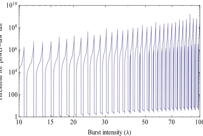
of power-law behaviour. The resulting estimate is shown in Figure 5.

10 15 20 30 50 70 100 1

100 104 106 108 1010

Burst intensity_

T

hr

es

ho

ld

fo

r

po

w

er



la

w

ta

il

Fig. 5. Lower bound for the threshold for power-law behaviour of the tail, in Mbytes (δ=1 second, r=1 Mbyte/s,γ=1.5,C=λγδ_γ−1r+3σ1, whereσ2₁is the variance of the number of bytes arriving in one second in the PPBP input process), computed by solving (26)=(24) by the Secant method.

will occur by a joint contribution of long and short bursts – hence the threshold, x_h, where power-law behaviour begins, becomes very large. In addition, even if we only consider systems where the capacity of the server,C, exceeds the arriving traffic by nearlyr, x_h increases steadily as λ−→∞. Because the estimate of x_h shown here is a lower bound on power-law behaviour, no significance should be given to the teeth projecting downward in Figure 5.

6 Comparison of approximations

6.1 The weight of the power-law tail

Expressions for the weight of the power-law tail provided in [6, 15, 28] (the result in [28] is appli-cable for a slightly different context), are difficult to evaluate numerically, except in the case where one burst is sufficient to overload the server.

Using the analysis of Subsection 4.3, and in particular equation (15), we obtain the approximation, which applies for largex:

lnP(Qt>x)∼ −η1(lnη1−lnβ) + (η1−β) (27)

whereη1=1+ j

C r −

λγ δ(γ−1)

k

is the least number of long bursts which cause an overflow of the buffer at threshold xwhen combined with the mean short burst load (we assume that the xis so large that virtually all bytes are in short bursts) andβis the mean number of long bursts (which will be defined more precisely in a moment).

The duration, τ, of this event leading to the overflow must stand in a simple relationship to the buffer threshold reached in the overflow,x, namely:

τ= x

rη1−C+λ_γ−rγδ₁

, (28)

because, whenxis large, the short burst component of the probability to be maximised rapidly moves from zero to one asτincreases in the near vicinity ofx/(rη1−C+λ_γ−rγδ₁). Putting this more directly:

the large bursts in combination with the short bursts are supplying work at a rate rη1−C+λ_γ−rγδ₁ in

excess of the servers capacity, during this overflow event. Therefore, the simplest, and most likely, way for the overflow to occur is for the buffer to start empty, and fill at this rate, until it reachesx. This will therefore happen over a period of timeτ, as defined at (28).

From this we conclude that the “long bursts” are all the bursts longer thanτand therefore the mean number of long bursts isβ= λτ

1−γ

δ(γ−1). From (27), therefore

lnP(Q_t>x)∼ −η1

lnη1−ln

λτ1−γ δ(γ−1)

+η1−

λτ1−γ δ(γ−1)

∼ −η1

lnη1−ln

λτ1−γ δ(γ−1)

+η1, (29)

because for largex,τis also large and so ln(τ1−γ)is large in magnitude, whereasτ1−γ→0.

Exponentiating both sides of (29) gives:

P(Qt>x)≈cλx

η1(1−γ)_{, (30)}

where

c_λ= η

−1

1 eλ

δ(γ−1)

!η1

rη1−C+

λrγδ

γ−1

−η1(1−γ)

(31)

This asymptotic formula is consistent with known results as regards thedecay; a formula for the

weightof the tail has been provided in [6], however equivalence of these two formulae is not clear and numerical evaluation of the formula in [6] has not been demonstrated in [6] or attempted here. The context in [6] is significantly different from here, so deducing a specific form, from this result, for the weight of the tail which applies in the present case would be difficult. This formula is also consistent with [27] in regard to the decay but because the latter formula is a heavy-traffic approximation the

weightof the tail is not comparable to the weight given here. The derivation ofc_λrelies on an assump-tion that events in which a coincidence of long bursts overload the linkoverlapis sufficiently rare that its probability can be neglected. For sufficiently heavy traffic this is not the case, so the formula given here forc_λcannot be expected to be consistent with the heavy traffic result in [27].

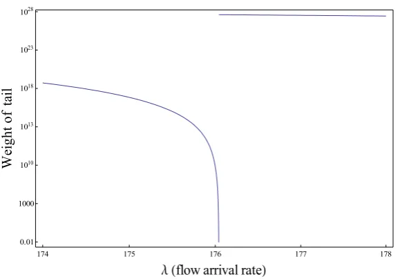
Plots ofc_λvsλare shown in Figures 6 and 7. From these graphs it seems that the weight of the large buffer asymptote can vary between 0 and 1028 over a very small range of λvalues. As λincreases fromr×kbelow server capacity tor×(k−1)below server capacity, the weight of the tail associated with events where there are preciselyk long bursts, gradually reduces to zero. The behaviour of c_λ

shown in Figures 6 and 7 is an essential feature of this system, not a numerical aberration.

1 5 10 50 100 500 1000

1085 1050 1015 1020 1055 1090

flow arrival rate

W

ei

gh

t

of

tai

l

Fig. 6. Weight of Large Buffer Asymptote as a function ofλ(broad view)

6.2 Comparison of the heavy traffic limit, large buffer limit and QS approximation

A series of similar PPBP queueing systems, with increasing burst rates, have been analysed by three methods (large buffer asymptote, heavy traffic Gaussian approximation, and QS approximation) and the results are shown in Figure 8. The parameters of the models under consideration in this figure areγ=1.5,δ=0.2 [seconds],r=1 [Mbit/sec] and λν=1, 64, and 32000 [bursts/sec]. The server

capacity,Cν, for each model has been adjusted so that the net mean,Cν−λ_γ−νr₁δ, and the autocorrelation

174 175 176 177 178 0.01

1000 1010

1013

1018

1023

1028

flow arrival rate

W

ei

gh

to

f

ta

il

Fig. 7. Weight of Large Buffer Asymptote as a function ofλ(close view)

The capacities of the three systems compared in Figure 8 have been set to λkrδγ γ−1 +

3σ_δ(λk,γ,δ,r)

δ . The

server rates which emerge from this calculation are: 2.79089, 55.9271, and 19591.9 Mbit/s.

Because Gaussian systems include, in general, significant amounts of “negative” traffic, the concept of system utilization is not meaningful for them. Instead, it is preferable to use the net meaninput. For this reason, even for PPBP systems, the net mean input, expressed in standard deviations over a certain time period, is a more meaningful parameter than system utilization for characterizing system behaviour. However, the system utilization is nevertheless of interest, particularly so that we can observe the gain in system efficiency as traffic load increases. The utilizations of the three systems shown in Figure 8 areλkrδγ

γ−1

/λkrδγ

γ−1 +

3σδ(λk,γ,δ,r)

δ

,k=1, 2, 3, which turns out to be 21.5%, 69%, and 99%, respectively.

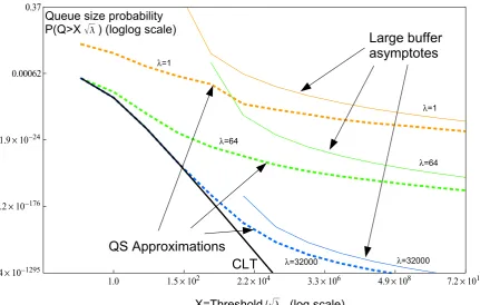
Figure 8 shows clearly that the quasi-stationary solution method is consistent with the Gaussian limit and with the large buffer limit. Although the large buffer asymptote appears to be an upper bound for the three choices of λdisplayed in Figure 8, cases where the large buffer asymptote are not an upper bound have also been observed in other experiments. This graph is plotted using log-of-log scale for the Y axis and a log-of-log scale for the X axis. These scales enable us to see results over a very wide range. The horizontal axis extends to buffer sizes up to 1010×√λ. The Y axis extends to probabilities as low as 10−1000. This range has been used so that the relationship between the different asymptotic regimes can be seen clearly. Calculating estimates by the different methods over such a wide range of parameter values is quite challenging and cannot be achieved without special effort.

The figure shows clearly the convergence of the queueing model to a limiting behaviour of a queue fed by Gaussian noise, which is also shown in the figure. The Gaussian model, with exactly the same autocorrelation as this PPBP, has been analysed in [30]. The method derived in that paper has been used here to compute the stationary distribution.

obtained as the large-deviations limit for the buffer distribution of a system handling this traffic, the resulting straight line curve would appear in almost the same position as the curve labelled CLT.

Plots of this type for a wider range ofλ values have shown that for Poisson arrival rates greater than about 4000 per second, a Gaussian model should be satisfactory. This figure for when a Gaus-sian model becomes satisfactory will depend critically upon assumptions concerning expected perfor-mance, the rate of each burst, and so on.

1.0 1.5102 _2.2104 _3.3106 _4.9108 _7.21010

2.4101295 6.210176 1.91024 0.00062 0.37

Large buffer asymptotes

QS Approximations CLT

X=Threshold (log scale)

λ=1

λ=32000

λ=1

λ=64

λ=32000

Queue size probability P(Q>X ) (loglog scale)

λ=64

/



Fig. 8. The stationary CDF as a function of buffer threshold for varying burst arrival rates (λ), estimated by QS algorithm, large buffer asymptote, and the CLT limit;C=mean traffic+3σ_δ/δ; buffer thresholds are measured in units of

√

λ.

Figure 8 clearly demonstrates how the heavy trafficandlarge buffer limits can apply despite appear-ing to lead to contradictory conclusions since, although the CDF’s clearly converge to the Gaussian result asλgrows, each one individually exhibits a completely different tail behaviour (which we know to be power-law).

6.3 Comparison with the many sources limit

Large Deviations Theory has been applied in two different ways to the system under study in this paper. One of these approaches was discussed in the previous subsection. The other approach has been used in [10, 15, 17–19, 32–34]. In this approach the limit is taken asn−→∞wherenis the number of sources, and the buffer threshold is assumed to grow in linear proportion tonalso.

Figure 1 of [10]. The many sources result diverges from the results of the present paper very sig-nificantly for any non-zero buffer threshold. Since the many sources approximation lies below the quasi-stationary approximation, which is itself a lower bound, it is clear that the discrepancy reveals a problem with the many sources large deviations result. To further emphasize the fact that the many sources approximation is clearly an underestimate, forx>0, we have included the stationary distri-bution for an FBN queueing system in this figure as well. The FBN input was chosen so that the input process had the same Hurst parameter as the PPBP process and the same variance at the time interval δ, which is equal to 0.2 in this instance. We expect, from experience with simulations for example [2], that the FBN system will exhibit better performance than the PPBP system. However, the many sources approximation exhibits better performance than the FBN system, which, in turn, is better than the quasi-stationary approximation.

It might be hoped that the difficulties of finding a satisfactory solution for the PPBP queue by the large buffer large deviations asymptotic approximation could be addressed by using the many sources asymptote instead. However, the many sources and the large buffer large deviations results must be consistent to a fairly high degree. As a consequence, the fact that the tail behaviour of the stationary queue distribution is not typical of practical buffer thresholds is forced to be a feature of the many sources approximation as well, for any buffer threshold greater than zero.

1.0 1.5102 _2.2104 _3.3106 _4.9108

3.51065

1.91024

1.9109

0.00062 0.066

Thresholdx log scale

P



Q



x



lo

g

sc

al

e



Duffield

model [10] QS Estimate

FBM

Fig. 9. Comparison with the many sources large deviations results.

7 Concluding remarks

The M/G/∞traffic model can be further improved, by allowing more complex behaviour for the individual bursts. Such an extension is natural to consider and the methods of this paper appear to be readily applicable to such models.

Appendix A: Overflow ProbabilityP(Q>x)and Loss ProbabilityP_loss(x)

As observed in [50], for the N∗D/D/1 queue and its finite buffer N∗D/D/1/xequivalence, thatP(Q>

x)provides an upper bound onP_loss(x)as follows:

P_loss(x)≤P(Q>x)

ρ (32)

whereρis the ratio of the mean arrival rate, denotedE(A), to the service rateC. In [29], it is shown that (32) applies also to the G/D/1 queue and its finite buffer equivalence. This observation was based on the definition of theoverflow period which is a maximal continuous period of time that the event

Q>xoccurs. Following [50], it can be shown that (32) applies also to the PPBP queue and its finite buffer equivalence. Since the PPBP queue size Q in the infinite queue system is the same at the beginning as at the end of the overflow period, the amount of work that joined the queue during an overflow period must be equal to the the amount of work served during the overflow period. Suppose ε>0 is arbitrary. Then, for sufficiently largeLt >0, the mean amount of work lost in the finite buffer PPBP queue (with buffer size x) during L_t is in the interval (E(A)L_tP_loss−ε,E(A)LtPloss+ε). This must be lower or equal to the amount of work thatarrivedduring the overflow period of the infinite buffer PPBP queue which is equal, as discussed above, to the amount of work served during that overflow period. Therefore, since the processQ_t is stationary,

E(A)LtPloss−ε≤CLtP(Q>x).

Sinceε>0 was arbitrary, (32) follows.

Appendix B: Proof of Propositions 1–3

Asλ→∞, in propositions considered in this appendix, the parametersr, the rate associated with each burst, and C, the capacity of the server, are scaled with λ according to the formulae (17), as explained at the start of Section 5. The remaining parameters,δandγ of the system of PPBP traffic processes under consideration remain fixed.

Proposition 1 For any functions, A_λ, B_λ of λ, and any increasing function, f(λ), defined on [0,∞),

such that

A_λx−f(λ)_≤

φ_λ(x)≤B_λx−f(λ), (18)

for all x>x₀, necessarily, Bλ Aλ →∞

asλ→∞.

The proof relies on four lemmas which we state and prove prior to presenting the proof.

ε>0there exists x0>0such that for x>x0,

e−(D+ε)xγ−1 ≤P(Q>x)≤e−(D−ε)xγ−1, (33)

where

D=4λr

2_δγ_(3−γ)γ−2

(2−γ)3(γ−1)γ

µ3−γ_.

Proof

Since the PPBP variance-time curve,σ_t2, takes the form shown in (14), ast−→∞

σ2_t ∼

D

r2λt3−γδγ

(γ−1)(2−γ)(3−γ)

where

_D

(γ−1)(2−γ)(3−γ), and in fact, for typical parameter values, this term is dominant even for

relatively smallt. In particular, for anyε>0 there existt0>0 such that for allt>t0,

(

_D

D

Observe therefore that the limitg(c) =limt→∞ σ2t

c2_σ2 t/c

exists andg(c) =c1−γ_{,c>0. Now}

inf

c>0g(c)(c+µ)

2_/2=2(γ−1)(3−γ)γ

(3−γ)3(γ−1)γµ

3−γ_,

so, by [9, Theorems 2.1 & 2.2],

lim b→∞

σ2_b

b2lnP(Q>b) =−

2(γ−1)(3−γ)γ

(3−γ)3(γ−1)γµ

3−γ_.

That is to say, for anyε0>0 we can findb0>0 such that forb>b0,

−2(γ−1)(3−γ)

γ

(3−γ)3(γ−1)γµ

3−γ₋

ε0

b2

σ2_b <ln

P(Q>b)<

−2(γ−1)(3−γ)

γ

(3−γ)3(γ−1)γµ

3−γ₊

ε0

b2

σ2_b.

Using (34), therefore, for anyε00>0, there is anx0>0 such that forx>x0,

−2(γ−1)(3−γ)

γ

(3−γ)3(γ−1)γµ

3−γ

_D

ε00

xγ−1_<lnP(Q>x)<

−2(γ−1)(3−γ)

γ

(3−γ)3(γ−1)γµ

3−γ

_D

ε00

xγ−1

from which the assertion of the lemma follows by exponentiation.

Lemma 2 Given arbitrary B, D₁>D₂>0, β>0, for any K >0, x0>0, there exists xL >0such that

inf

λ,α>0x0≤supx≤xL

max αx

−λ

Be−D2xβ ,Be

−D1xβ

αx−λ

!

Proof

Essentially, this lemma says that a graph of the mapping x7→αx−λ is fundamentally different in shape to a graph of x7→Be−Dxβ, no matter how the parameters α, λ, B, D, and β are chosen. The detailed proof has been omitted in the interests of brevity, but can be found in the long version of this paper [48].

Lemma 3 The CDF of a Gaussian queueing system with non-zero idle probability is continuous on

(0,∞).

Proof

This result follows from Theorem 11 in [51, Section 11]. In [51] the main conclusion of Theorem 11 is that the CDF, F(r) say, is absolutely continuous on (r0,∞) where r0 =inf{r :F(r)>0}. In

[51],F(r)is the CDF of convex functional defined on an Gaussian process on an arbitrary index set whereas in the present case we shall apply this withF(r)as the CDF of

sup s≤t

X_t−X_s=X_t−X_St

whereS_tdenotes the time,s, previous totwhereX_t−X_sachieves its maximum value. As noted in the Corollary to Theorem 11 in [51], this sup is a convex linear functional, so Theorem 11 applies to it. In the present case,r₀=0, since the system has a non-zero probability of being idle.

Lemma 4 The sequenceφ_λ(x)converges to the CDF of the Gaussian queueing system whose input

process has the same first and second order statistics as the PPBP uniformly in x on any finite interval

in[0,∞), asλ−→∞.

Proof

Point-wise convergence follows from the CLT [8, 39] and Lemma 3. Choose a finite interval[a,b]⊆ [0,∞). Letφ(x) =lim_λ→∞φ_λ(x),x>0. This is a uniformly continuous function on[a,b](because[a,b] is compact). The rest follows from the fact that bothφ(x)and all theφ_λ(x), are increasing functions ofx.

Proof of Proposition 1

By Lemma 1, for anyε>0, for somex1>x0, (33) holds for all x>x1. We could chooseε=D/4

for example. LetD1=D+εandD2=D−ε, so, by (33), for allx>x1,

Ce−D1xγ−1 _{≤ψ(x)≤Ce}−D2xγ−1_{. (35)}

Now, by Lemma 2, we can find x_L > x₁ such that for any α, κ, for some x ∈ (x1,xL), either

αx−κ

Ce−D₂xγ−1 >K2or

Ce−D₁xγ−1

αx−κ >K

2_.

Applying this withB_λ forα, and f(λ)forκ, we see that over the rangex1toxL, the upper bound B_λx−f(λ)

λ must, for some value ofx, fail to approximate the functionsCe

−D1xγ−1 _andCe−D2xγ−1 _{by a}

ratio of at leastK2, i.e. for anyλ>0, we can findx_λ∈(x1,xL)such that either

B_λx−f(λ)

λ

Ce−D2xγ− 1 λ

>K2 (36)

or

Ce−D1xγ_λ−1

B_λx−f(λ)

λ

>K2. (37)

By Lemma 4, φ_λ(·) converges to its limit ψ(·) as λ→ ∞ uniformly on any finite interval of x values. So we can choose λK sufficiently large that for all λ>λK the ratioφλ(x)/ψ(x)>1/K and

ψ(x)/φ_λ(x)>1/K over(x1,xL). Using (35), we now see that for allλ>λK

Ce−D2xγ−1_/

φ_λ(x)>1/K (38)

and

φ_λ(x)/Ce−D1xγ

−1

>1/K (39)

over(x1,xL).

If (37) were to hold, multiplying it by (39) gives

B_λx−f(λ)

λ

φλ(xλ)

< 1

K,

forλ>λK, which contradicts the assumption thatBλx

−f(λ)

λ is an upper bound. Hence (37) does not

hold.

So (36) holds. Multiply it by (38) to give

B_λx−f(λ)

λ

φ_λ(x_λ) >

K

forλ>λK. SinceK >0 was arbitrary, this proves that

B_λx−f(λ) λ

φ_λ(x_λ) −→∞asλ−→∞ and hence, since

A_λx−f(λ)

λ <φλ(xλ), also that

B_λ

Proposition 2 In the same context as Proposition 1

For any mapping,λ7→B_λ, (orλ7→A_λ) and function, f(λ), defined on[0,∞), such that

φ_λ(x)≤B_λx−f(λ) (40)

A_λx−f(λ)≤φ_λ(x)

, (41)

for all x>x₀, necessarily, for any x₀>0,sup_x>x0 Bλx−f

(λ)

φ_λ(x) →∞(infx>x0

φ_λ(x)

A_λx−f(λ) →0) asλ→∞.

Proof

Selectx₀>0. Except that when we pickx₁, we need to select it to be larger than max(x0,x0), instead

of just larger thanx₀, the proof is the same as for Proposition 1 up to the penultimate conclusion. The

penultimate conclusion was thatBλx −f(λ)

λ

φ_λ(x_λ) −→∞asλ−→∞. Sincexλ>x1, it is also larger thanx0. The

primary statement of the proposition follows. The secondary statement follows by an entirely parallel argument.

Proposition 3 In the same context as Proposition 1, if A_λx−f(λ) _{is a power-law asymptote for a}

PPBP queue, in the sense that for any PPBP system, Aλx −f(λ)

φλ(x)

−→1as x−→∞, the convergence is not

uniform inλ. For any x0>0, eithersupx>x0 Aλx−f

(λ)

φ_λ(x0) −→∞orinfx>x0 Aλx−f

(λ)

φ_λ(x0) −→0asλ−→∞.

Proof

If it is not the case that infx>x0 Aλx

−f(λ)

0

φλ(x0) −→ 0 as λ−→∞, then for some K > 0, for all x >x0, Aλx−f

(λ)

φ_λ(x) >K. Then(K

−1_A

λx−f(λ))will be an upper bound satisfying the conditions of Proposition 2,

and therefore sup_x>x0K−1Aλx −f(λ)

φλ(x) →∞asλ→∞, from which the conclusion follows.

Acknowledgement

This work was supported by the Australian Research Council (ARC). The work on the paper was conducted when M. Zukerman was with the ARC Special Research Centre for Ultra-Broadband In-formation Networks, EEE Dept, The University of Melbourne, Australia.

References

[1] W. E. Leland, M. S. Taqqu, W. Willinger, D. V. Wilson, On the self-similar nature of Ethernet traffic (extended version), IEEE/ACM Trans. Networking 2 (1) (1994) 1–15.

[2] R. G. Addie, T. D. Neame, M. Zukerman, Performance evaluation of a queue fed by a Poisson Pareto burst process, Computer Networks 40 (2002) 377–397.