Traffic Flow Forecasting Based on Combination of Multidimensional Scaling and SVM

Traffic Flow Forecasting Based on Combination of Multidimensional

Scaling and SVM

a. Key Laboratory for Computer Network of Shandong Province, Shandong Computer Science Center, Jinan, Shandong, 250014, China

b. School of Informatics and Computing, Pervasive Technology Institute, Indiana University Bloomington,

Bloomington, Indiana, 47408, USA

Abstract: Traffic flow forecasting is a popular research topic of Intelligent Transportation Systems (ITS). With the development of information technology, lots of history electronic traffic flow data are collected. How to take full use of the history traffic flow data to improve the traffic flow forecasting precision is an important issue. More history data are considered, more computation cost should be taken. In traffic flow forecasting, many traffic parameters can be chosen to forecast traffic flow. Traffic flow forecasting is a real-time problem, how to improve the computation speed is a very important problem. Feature extraction is an efficient method to improve computation speed. Some feature extraction methods have been proposed, such as PCA, SOM network, and Multidimensional Scaling (MDS) and so on. But PCA can only measure the linear correlation between variables. The computation cost of SOM network is very expensive. In this paper, MDS is used to decrease the dimension of traffic parameters, interpolation MDS is used to increase computation speed. It is combined with nonlinear regression Support Vector Machines (SVM) to forecast traffic flow. The efficiency of the method is illustrated through analyzing the traffic data of Jinan urban transportation.

Keywords: Traffic flow forecasting, Multidimensional Scaling; SVM; Interpolation

1

Introduction

Short-time traffic flow forecasting is a popular research topic of Intelligent Transportation Systems (ITS). Correct traffic flow forecasting is the precondition of real-time traffic signal control, traffic assignment, route guidance, automatic guidance, and accident detection. The study of traffic flow forecasting is very significant in ITS. Many scholars have been studying on the topic and many forecasting models have been developed. Commonly used methods include average method, ARMA, linear regression, nonparametric regression, and neural networks [1-3]. The forecasting precisions of these methods usually can’t meet with the practical requirement. Support Vector Machines (SVM) is proposed by V. Vapnik in 1995[4]. It is a network model that is based on the principle of structure risk minimization and VC dimension theory. It can resolve small sample, nonlinear, high dimension, and local minimum problems efficiently [5]. SVM is mainly used to resolve classification and regression problems. Nonlinear regression SVM has been used to forecast traffic flow and obtained good results [6].

observations that are similar to one another are represented by points that are close together. It is a nonlinear dimension reduction method. But the computation complexity is 𝑂(𝑛2) and memory requirement is 𝑂(𝑛2). With the increase of sample size, the computation cost of MDS increase sharply. For improving the computation speed, interpolation MDS are introduced in reference [10]. It is used to extract feature from large scale traffic flow data. Nonlinear SVM is used to forecast traffic flow.

The following of the paper is organized as follows. Interpolation MDS method is introduced in part 2. Nonlinear SVM is introduced in part 3. Traffic flow forecasting procedure based on MDS and nonlinear SVM is introduced in part 4. A practical example is analyzed with the proposed model in part 5. At last some conclusions are summarized.

2 Interpolation MDS

2.1 Multidimensional Scaling

MDS is a non-linear optimization approach constructing a lower dimensional mapping of high dimensional data with respect to the given proximity information based on objective functions. It is an efficient feature extraction method. The method can be described as follows.

Given a collection of 𝑛 objects 𝐷= {𝒙₁,𝒙₂,⋯,𝒙_𝑛},𝒙_𝑖∈ 𝑅𝑁(𝑖= 1,2,⋯,𝑛) on which a distance function is defined asδ_i,j, the pairwise distance matrix of the 𝑛 objects can be denoted by

∆≔ �

𝛿

𝛿

𝛿

𝛿

⋯

𝛿

𝛿

⋮

⋱

⋮

𝛿

𝛿

⋯ 𝛿

�

whereδ_i,j is the distance between 𝒙_𝑖 and 𝒙_𝑗. Euclidean distance is often adopted.

The goal of MDS is, given Δ, to find𝑛 vectors 𝒑₁,⋯,𝒑_𝑛 ∈ 𝑅𝐿(𝐿 ≤ 𝑁) to minimization the STRESS or SSTRESS. The definition of STRESS and SSTRESS are as follows.

𝜎(𝑃) =∑ 𝑤𝑖<𝑗 𝑖,𝑗�𝑑𝑖,𝑗(𝑃)− 𝛿𝑖,𝑗�2 (1)

𝜎2_{(𝑃) =∑ 𝑤}

𝑖,𝑗�(𝑑𝑖,𝑗(𝑃))2− 𝛿𝑖2,𝑗�2

𝑖<𝑗 (2) where 1≤i < j≤n, 𝑤_𝑖,𝑗 is a weight value (𝑤_𝑖,𝑗 > 0), 𝑑_𝑖,𝑗(𝑃) is a Euclidean distance between mapping results of 𝒑_𝑖 and 𝒑_𝑗. It may be a metric or arbitrary distance function. In other words, MDS attempts to find an embedding from the 𝑛 objects into 𝑅𝐿such that distances are preserved.

2.2 Interpolation Multidimensional Scaling

One of the main limitations of most MDS applications is that it requires 𝑂(𝑛2) memory as well as O(n2_{) computation. It is difficult to process MDS with large scale data set because of the limitation of} memory limitation. Interpolation is a suitable solution for large scale MDS problems. The process can be summarized as follows.

Given n samples data 𝐷= {𝒙₁,𝒙₂,⋯,𝒙_𝑛},𝒙_𝑖 ∈ 𝑅𝑁(𝑖= 1,2,⋯,𝑛) in N dimension space, m samples

𝐷𝑠𝑠𝑠 = {𝒙1,𝒙2,⋯,𝒙𝑚}, are selected to be mapped into L dimension space 𝑃𝑠𝑠𝑠 = {𝒑1,𝒑2,⋯,𝒑𝑚} with MDS. The other samples 𝐷_{𝑟𝑠𝑠𝑟} = {𝒙₁,𝒙₂,⋯,𝒙_𝑛−𝑚}, will be mapped into L dimension space 𝑃_{𝑟𝑠𝑠𝑟} = {𝒑1,𝒑2,⋯,𝒑𝑛−𝑚} with interpolation method. The computation cost and memory of interpolation MDS is only 𝑂(𝑛). It can improve the computing speed markedly.

After data set 𝑄 being selected, the mapped value of the input sample is calculated through minimizing the following equations as similar as normal MDS problem with 𝑘+ 1 points.

𝜎(𝑋) =∑ �𝑑𝑖<𝑗 𝑖,𝑗(𝑃)− 𝜹𝒊,𝒋�2=𝐶+∑ 𝑑𝑘𝑖=1 𝑖𝑖2 −2∑ 𝑑𝑘𝑖=1 𝑖𝑖𝛿𝑖𝑖

(3)

In the optimization problems, only the position of the mapping position of input sample is variable. According to reference [10], the solution to the optimization problem can be obtained as

𝑥[𝑟]_=𝒑�+1

𝑘∑ 𝛿𝑖𝑖

𝑑𝑖𝑖�𝑥

[𝑟−1]_{− 𝒑}

𝑖� 𝑘

𝑖=1 (4)

where 𝑑_𝑖𝑖=�𝒑_𝑖− 𝑥[𝑟−1]� and 𝒑� is the average of k pre-mapped results. The equation can be solved through iteration. The iteration will stop when the difference between two iterations is less than the prescribed threshold values. The difference between two iterations is denoted by

𝛿 =(�𝑖_�𝑖[𝑡]−𝑖[𝑡−1[𝑡−1]_�]�) (5)

3 Support Vector Machines

SVM first maps the input points into a high-dimensional feature space with a nonlinear mapping function Φ and then carry through linear classification or regression in the high-dimensional feature space. The linear regression in high-dimension feature space corresponds to the nonlinear classification or regression in low-dimensional input space. The general SVM can be described as follows.

Let l training samples be T ={(x1,y1),,(xl,yl)}, where

n X

i R

x ∈Ω = , yi∈ΩY =R, i=1,,l.

Nonlinear mapping function is k(xi,xj)=Φ(xi)⋅Φ(xj). Nonlinear regression SVM can be implemented

through solving the following equations.

min 𝛼∗_∈𝑅2𝑙

1

2 �(𝛼𝑖∗− 𝛼𝑖)�𝛼𝑗∗− 𝛼𝑗�𝑘�𝑥𝑖.𝑥𝑗� 𝑠

𝑖,𝑗=1

+𝜀 �(𝛼𝑖∗+𝛼𝑖) 𝑠

𝑖=1

− � 𝑦𝑖(𝛼𝑖− 𝛼𝑖∗) 𝑠

𝑖=1

𝑠.𝑡.∑𝑠𝑖=1(𝛼𝑖− 𝛼𝑖∗)= 0 (6)

𝛼𝑖,𝛼𝑖∗≥0 ∀𝑖= 1,⋯, l

Through optimization, optimum solution α(*)=(α₁,α₁*,,α_l,α_l*)can be solved.

Select the positive sub-vector α_j >0 of α or the positive sub-vector α*

of α*j >0 and calculate the parameter

ε α

α − −

− =

∑

j K x x

y b 1 * ) , ( )

( (7)

After getting the optimum parameters, the decision function can be denoted as

∑

i k x x b

x f 1 * ) ( ) ( )

( α α (8)

It is very important to choose appropriate kernel function of SVM. The kernel function must satisfy the Mercer condition. At present, many kernel function model have been developed. Commonly used kernel functions include

(1) linear: 𝐾�x_𝑖, x_𝑗�= x_𝑖𝑇x_𝑗

(3) radial basis function (RBF): 𝐾�x_𝑖, x_𝑗�= exp (−𝛾�x_𝑖−x_𝑗�2),𝛾> 0

(4) sigmoid: 𝐾�x_𝑖, x_𝑗�= exp (−𝛾�x_𝑖−x_𝑗�2),𝛾> 0 Here, 𝛾,𝑟,𝑎𝑛𝑑𝑑 are kernel parameters.

4 Traffic Flow Forecasting

In intelligent transportation system, many traffic flow parameters are useful in identifying the traffic state, such as speed, traffic flow volume, and time occupancy and so on. Short term forecasting of the parameters is the precondition of

providing traffic information services. In the forecasting of the traffic flow parameters, many traffic flow data can be used, such as the previous sampling data, history cycle data and so on. The included data should be prescribed previously according

to practical requirement and experience. Traffic flow forecasting model is built according to history traffic flow data. Training samples can be generated according to the model. Sample data are mapped into low dimension space with MDS method. Traffic flow data are forecasted based the mapped data with SVM. The method is summarized as follows.

1) Generate samples

Firstly, determine the feature vector 𝑥= [𝑥₁,𝑥₂,⋯,𝑥_𝑁], 𝑁 is the number of selected traffic flow data. Current time traffic flow data to be forecasted is denoted by 𝑦. Samples can be generated according to the model with history traffic flow data.

2) Dimension reduction

Select some samples and mapped them into low dimension space with MDS methods introduced as in section 2.1. Prescribe the number 𝑘 of nearest neighbors. The other samples are mapped into low dimensions with interpolation method

introduced as in section 2.2.

3) Traffic flow forecasting with SVM

All the mapped samples are divided into two parts. One part is used to train nonlinear SVM model. The other is used to

test the trained model. Some indices can be used to evaluate the training model in quantitatively. Commonly used are following three indices.

(1)Mean absolute percentage error (MAPE)

𝑀𝑀𝑃𝑀=1_{𝑛 � �}𝑦�𝑖_𝑦− 𝑦𝑖

𝑖 � 𝑛

𝑖=1

(2) Mean absolute error (MAE)

𝑀𝑀𝑀=1_{𝑛 �}|𝑦�𝑖− 𝑦𝑖| 𝑛

𝑖=1

(3) Mean square error (MSE)

𝑀𝑀𝑀=1_{𝑛 �}(𝑦�𝑖− 𝑦𝑖)2 𝑛

𝑖=1

where n is the number of test samples, yˆi is the forecasting value, and yi is the detected value.

5 Example

5.1 Data source

Jinan traffic police branch provides us with traffic flow data and video data of Jingshi Road expressway. Through the express way, there are about 14 intersections. The traffic flow data are collected by inductance loop vehicle detectors. We

select traffic flow data of the cross between Jingshi road and Lishan Road from June 1, 2007 to July 1, 2007 to study. In the intersection, there are four directions. We select the direction from west to east. Data collecting equipment is loop detectors which can detector three traffic parameters, i.e. volume, average speed and occupancy. Collecting interval is 5 minutes. There

5.2 Generate samples

Traffic flow parameter value to be forecasted is denoted by variable Y. Traffic flow parameter value of current cross

at previous sampling times are denoted by variable vector ( , , , )

1

2

1 X XN

X 

=

X where Xi,i=1,2,,N₁ denotes previous i sampling time value. Traffic flow parameter value of current cross at history times are denoted by variable

vector ( , , , )

2

2

1 H HN

H 

=

H where Hi,i=1,2,,N2 denotes previous i days’ time value. 𝑿= [𝑿,𝑯] is taken as

the feature vector.

In this example, N₁= 10 previous sampling time data and N₂= 5 history sampling data are prescribed. The history cycle is set 1 day. For generating samples, 5 days history data should be retained. 51747 samples are generated in the end. 5.3 Dimension reduction

In this example, 4000 samples are selected to be pre-mapped into low dimension space. Firstly, calculate the distance matrix. Euclidean distance is adopted here. Then calculate the mapped vector according to the distance matrix with MDS

method. The others are mapped into low dimension with interpolation MDS method. The number of nearest neighbor is set 𝑘= 10. For comparison, the dimension number is set as 2, 3, and 5 respectively.

5.4 Forecasting with SVM

After selecting the independent variables, we take them as the input and variable Y as the output of SVM respectively. We select 31048 samples randomly as the training set to train the SVM and 20699 samples as the testing set.

The computation configuration is as follows. The operation OS is Ubuntu Linux. The processor is 3GHz Intel Xeon with 8GB RAM. Based on different feature dimension number, the training time of SVM is compared. For illustrate the

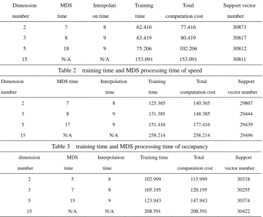
efficiency of feature extraction, we train the SVM with all feature variables, i.e. no feature extraction. The training time based on 2, 3 ,5 and 15 feature dimensions are listed in table 1, table 2 and table 3. They corresponds to traffic parameter volume, speed and time occupancy respectively.

Table 1 training time and MDS processing time of volume

Dimension

number

MDS

time

Interpolati

on time

Training

time

Total

computation cost

Support vector

number

2 7 8 62.416 77.416 30873

3 8 9 63.419 80.419 30817

5 18 9 75.206 102.206 30812

15 N/A N/A 153.091 153.091 30811

Table 2 training time and MDS processing time of speed

Dimension

number

MDS time Interpolation

time

Training

time

Total

computation cost

Support

vector number

2 7 8 125.365 140.365 29807

3 8 9 131.385 148.385 29444

5 17 9 151.416 177.416 29439

15 N/A N/A 258.214 258.214 29496

Table 3 training time and MDS processing time of occupancy

dimension

number

MDS

time

Interpolation

time

Training time Total

computation cost

Support

vector number

2 5 8 102.999 115.999 30318

3 7 8 105.195 120.195 30255

5 15 9 123.943 147.943 30374

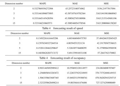
After training SVM model, the left samples are used to test. The test results of traffic parameter volume, speed, and occupancy are listed in table 4, table 5 and table 6 respectively.

Table 4 forecasting result of Volume

Dimension number MAPE MAE MSE

2 0.3327869556272506 43.25723160574062 3156.21977017094

3 0.3331461896075895 43.307107619782364 3163.0419818868963

5 0.3331645145428394 43.308562765106906 3163.2133145681196

15 0.333166210665571 43.308546054378546 3163.2080066138265

Table 4 forecasting result of speed

Dimension number MAPE MAE MSE

2 0.13492261616445286 4.603466040475783 37.404266352045425

3 0.13976340327264516 4.80394551521134 42.19170567536615

5 0.15201120462250647 5.326185736608295 51.37989843956938

15 0.16030626203713172 5.691339918531108 57.2843762170002

Table 4 forecasting result of occupancy

Dimension number MAPE MAE MSE

2 0.9031465692989412 10.550692120114977 234.8826008707607

3 1.2560058543283672 13.228337925210955 370.73752698149553

5 1.5063358633687365 15.040251159308761 470.56202943254715

15 2.3232558620498214 19.88356441476406 727.3274250880689

5.5 Results analysis

The computation cost of training time and MDS processing time are shown as in figure 1. From the analysis results we can find the computation cost can be decreased markedly with the decrease of dimension number. It illustrates that feature extraction is efficient in traffic flow forecasting.

Figure 1 computation time based on different dimension number

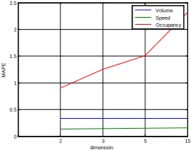
The test results of different traffic parameters are shown as in figure 2, 3 and 4. From the results we can find that the forecasting precision will not decrease with the reduction of dimension number. It is mainly because that the traffic data have

noise. Feature extraction can filter the noise efficiently. It can improve the forecasting precision.

2 3 5 15

0 50 100 150 200 250 300

dimension

c

om

put

at

ion t

im

e

Figure 2 MAPE of forecasting results

Figure 3 MAE of forecasting results

Figure 4 MSE of forecasting results

6 Conclusions

How to improve the forecasting precision of traffic flow is still an important topic in intelligent transportation systems because of the complexity and nonlinear character. In this paper we proposed to combine MDS with nonlinear SVM to

forecast traffic flow data. The MDS is used to decrease the input feature vector dimension. Interpolation MDS is used to improve the dimension reduction speed. The example analysis results show that the proposed method can improve the forecasting speed. At the same time, the forecasting precision can be improved through filtering the noise in the traffic flow

data. It illustrates that the proposed method is efficient in traffic flow forecasting.

Acknowledgements

This work is partially supported by Provincial Outstanding Research Award Fund for young scientist (No. BS2009DX016) and Provincial Fund for Nature project (No. ZR2009FM038).

References

1 Yang Zhaosheng. Basis traffic information fusion technology and its application. Beijing, China Railway Publish House, 2005.

2 Wang, Fan, Tan Guo Zhen, Deng Chao. Parallel SMO for Traffic Flow Forecasting. Applied Mechanics and Materials, 2010, Vol. 20

Issue: 1 p843-848

3 Stephen Clark. Traffic Prediction Using Multivariate Nonparametric Regression. Journal of Transportation Engineering, 2003, 129(2):

161-168.

4 Cortes C, Vapnik V. Support Vector Networks[J]. Machine Learning, 1995, 20: 273–297.

5 C.-C. Chang and C.-J. Lin. LIBSVM : a library for support vector machines. ACM Transactions on Intelligent Systems and Technology,

2 3 5 15

0 0.5 1 1.5 2 2.5

dimension

M

APE

Volume Speed Occupancy

2 3 5 15

0 5 10 15 20 25 30 35 40 45

dimension

MA

E

Volume Speed Occupancy

2 3 5 15

0 500 1000 1500 2000 2500 3000 3500

dimension

MS

E

2:27:1--27:27, 2011.

6 Hong, Wei-Chiang. Application of seasonal SVR with chaotic immune algorithm in traffic flow forecasting. Neural Computing &

Applications; Apr2012, Vol. 21 Issue 3, p583-593

7 Jolliffe, I. T. Principal component analysis. New York : Springer, 2002.

8 George K Matsopoulos.Self-Organizing Maps. INTECH, 2010.

9 Borg Ingwer, Patrick J.F. Croenen. Modern Multidimensional Scaling: Theory and Applications. New York : Springer, c2005. pp. 207–

212

10 Seung-Hee Bae, Judy Qiu, Geoffrey Fox Adaptive Interpolation of Multidimensional Scaling International Conference on