Abstract: This paper brings out an outlook of atmospheric contamination and its strategies to predict the nature of atmosphere. Air Pollution Modeling (APM) is being created and utilized to comprehend, explore, evaluate, and control the nature of the atmospheric condition and the dispersion of lethal toxins. It includes viewpoints identified with the existence cycle of pollutants, beginning from their emanation or 'creation' inside the climate, and consummation with their effects on man and the biological system. This provides a general review of the best in class on air quality demonstrating, from the perspective of the 'client network', which comprises of approach producers, urban organizers, natural administrators, and etc. The investigation includes simulation and modeling of contamination information. Models like Non-receptive (e.g., Gaussian plume models) and responsive (e.g., photochemical models) are talked about.
Key Words: Atmospheric contamination, modeling, Gaussian plume models, air quality, photochemical models.
I. INTRODUCTION
Air contamination models use logical and numerical method to assess the physcio -chemical process that impact air toxins as they dissipate and act in the climate.In light of meteorological data and source information like release rates and stack height, these models are proposed to depict the contaminations that are discharged straightly into nature and, now and again, auxiliary pollutants that are shaped on account of complex substance reactions inside the environment.These models are fundamental to our air quality management framework since they are usually utilized by agencies entrusted with controlling air contamination to both recognize source commitments to air quality crisis and encourages in the plan of successful systems to minimizeharmfulatmosphericpollutants. For instance, air quality models can be utilized to check that a new source won't surpass encompassing air quality measures or, if important, decide reasonable additional control measures. Furthermore, air quality models can likewise be utilized to foresee future toxin fixations from various sources after the execution of another regulatory program, to rough the viability of the program in decreasing harmful exposures to people and the environment. The most utilized air quality models incorporate the accompanying:
Revised Manuscript Received on June 05, 2019
Laxmipriya.S, Research Scholar, Department of Civil Engineering,Dr. M.G.R. Educational and Research Institute, Chennai, India & (Assistant Professor, Panimalar Engineering College, Chennai, India).
Dr.NARAYANAN.RM, Professor, Department of Civil Engineering Dr. M.G.R. Educational and Research Institute, Chennai, India
Dispersion Modeling - These models are utilized in the allowing procedure for evaluating the grouping of toxins at indicated ground-level receptors surrounding an emission source.
Photochemical Modeling –These models are ordinarily used in authoritative or technique evaluations for reenacting the impacts from all sources by assessing pollutant concentration and testimony of both inactive and falsely responsive toxins over enormous spatial scales.
Receptor Modeling - These observational models use the chemical and physical character of gases and particles evaluated at source and receptor for recognizing the presence and quantifying the source and receptor concentrations.
II.SOURCES OF AIR POLLUTION
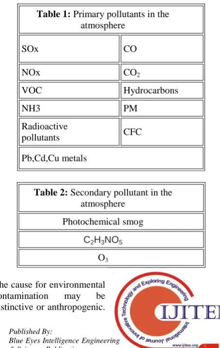
[image:1.595.312.539.468.826.2]The substances causing air contamination are together known as air toxins. They might be strong, fluid or vaporous in nature. Contaminations are named primary and secondary air pollutants. Primary contaminations are radiated legitimately to environment, though, secondarypollutants are formed through chemical responses and different blends of the primary pollutants. Some important primary and secondary air pollutantslisted below
Table 1: Primary pollutants in the atmosphere
SOx CO
NOx CO2
VOC Hydrocarbons
NH3 PM
Radioactive
pollutants CFC
Pb,Cd,Cu metals
Table 2: Secondary pollutant in the atmosphere
Photochemical smog
C2H3NO5
O3
The cause for environmental
contamination may be
distinctive or anthropogenic.
Laxmipriya.S,Narayanan.Rm
The anthropogenic contaminants are those caused by human movement. The major anthropogenic sources includestationary sources, (for example, smoke heaps of intensity plants, incinerators, and heaters), transportable sources (for example vehicular and airplane), agriculture and industry (for example synthetic compounds and dust), fumes from paint, hair splash, vaporized showers, landfills (which contain methane) and military (for example atomic weapons and lethal gases). The natural sources of atmospheric contamination might be due dust emission along low vegetation regimes, radon gas from radioactive rot of earth crust, smoke emanated from control fires, and volcanic eruptions which produces sulfur, chlorine and particulates.
III.APPLICATIONS OF AIR-POLLUTION MODELS
Providing a thorough outline of all application cases for air pollution models is unimaginable here. , overall air-pollution modeling can be sorted by:
• Spatial goals—worldwide, local, nearby/urban scale • Model idea—Lagrangian, Eulerian, or CFD
• Model type—simple dispersion models or complex chemistry transport models
• Application—ex-post evaluation or
Projection/gauging of contamination occasions
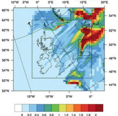
[image:2.595.50.253.584.784.2]Air-contamination models are generally utilized by national and local authorities to evaluate consistence with air-quality point of confinement esteems (ex-post), just as to measure the effect of conceivable future improvements (e.g., for regulatory purposes for ex-ante ecological effect appraisals). In this specific situation, models are connected to supplement existing estimations or to evaluate focuses or testimonies in territories where no observing destinations exist (for this situation, progressively complex models can give increasingly precise portrayals of complex fixation or testimony fields than interpolation procedures)Figures 1and 2 provide examples of the analysis of air pollution using atmospheric chemistry transport models and serve to illustrate the abundance of applications of air-pollution models at different scales and for different purposes
Figure 1. Application of a regional atmospheric chemistry transport model over the United Kingdom (EMEP4UK) showing surface concentrations of nitrogen dioxide (NO2) at different spatial scales and resolutions.
Figure2. Global model forecast of ozone surface concentrations provided by the Monitoring Atmospheric Composition & Climate (MACC) project
IV.AIR POLLUTION MODELING
Air pollution models provide a contributory connection between releases, climatology, atmospheric deposition and diverse variables. They clarify the outcomes of past and future situations and the determination of the effectiveness of abatement methodologies. Which is additionally used to portray the convergence of different pollutants all around. The major sorts of air pollution models are discussedbelow.
GAUSSIAN PLUM MODEL
This is an essential numerical model used to evaluatethe grouping of pollutants at a point from the source of outflow. This model is utilized for static just as transportable sources of emanations. In this model, the scattering in the three dimensions is determined. Scattering along the downwind direction is a constituent of mean breeze speed blowing across the plume.Air contamination is articulated by an overestimated crest originating from the top of a stack of some height and diameter.The noteworthydisadvantage of this model is prevailing oflonger timeframes of the steady state conditions with reference to pollutant emissions andmeteorological changes. The model is used to ascertain the effective stack height, lateral and vertical dispersion coefficients and ground-level concentrations. The Gaussian plum model is delineated in the figure
underneath. The model was planned by
determiningexperimentally the horizontal and vertical spread of the plume, estimated by concentration distribution of dispersion plumes.
The AERMOD is the next generation air dispersion model dependent on planetary limit layer hypothesis. AERMOD uses a comparative information and yield structure to ISCST3 and offers considerable similar highlights, just as offering extra highlights. AERMOD completely consolidates the PRIME structure downwash calculations, progressed depositional parameters, neighborhood territory impacts, and progressed meteorological turbulence computations.
Examinations gave the geometrical depiction of the plume by plotting the standard deviation of its concentration distribution, in both the vertical and level course, as a part of the barometrical soundness and downwind detachment from the source. The plotting is exhibited in the figure underneath
EULERIAN AND LAGRANGIAN MODEL
An Eulerian dispersion model explains a conservation equation for vaporous or airborne materials, which can be communicated formally extremely simple and which can be changed into an exceptionally quick numerical code. Then again, Eulerian dispersion modeling is frequently dismissed due to the presence of artificial diffusion. Utilizing the Lagrangian approach, directions of many particles must be determined in little sequential time steps. Each molecule conveys a specific measure of vaporous or airborne mass. The movement of the molecule is controlled by normal wind speed segments and turbulence conditions. The latter is portrayed scientifically by a Markov procedure. Concentration is determined by tallying particles or time-interims of particles inside the grid volumes. Artificial numerical dispersion does not happen by utilizing this technique, in any case, since measurement exactness is imperative,
more often than not an immense number of molecule directions must be determined, which may prompt very tedious time-consuming simulations, particularly, when low work width relate with an expansive model space.
Software utilized: •AUSTAL2000
AUSTAL View is anair dispersion modeluses graphical UI of Germany’s Federal Environmental Agency, created by atmosphericpollution control guideline TALuft(TechnicalInstructionsonAir Quality). It is a Lagrangiandispersion model consisting indigenous wind field model (TALdia). TheAUSTAL View model contemplates the impact of geography on the wind field and subsequently on the dispersion of pollutants in the atmosphere.
CALPUFF MODELS
Calpuff models were acquainted to simulate the conduct of contaminations in inhomogeneous and non-stationary meteorological and emission conditions. The outflow is discretized in a transient progression of puffs, every one of which shifts into the region of math on account of wind field. Puff models accept that every outflow of pollutants discharges into the environment is variable in time. Each puff contains the mass M and its focal point of mass is transported by the wind, which may change in reality. Constantly emitting sources can be represented by the superposition of a progression of the above mists. The puffs considered here are radiated in time interims1 and the computation of the grouping of pollutants of each one is set aside a time interval2. Each puff is conveyed as per the direction from its middle, which is resolved for speed vector of the neighborhood wind, while it is developed in the time by means of dispersion coefficients.
Software’s utilized: • USEPA Version 5.8 • USEPA Version 6 • USEPA Version 7
USEPA gives a total graphical answer for the CALPUFF
modeling framework: CALPUFF, CALMET,
CALPOST, and their related pre-and post-processors. USEPA incorporates powerful and free QA tools, dazzling report-prepared outcomes, and a wide scope of representation alternatives
PHOTOCHEMICAL MODELS
Photochemical models are normally utilized in administrative or policy appraisals to simulate the effects from all sources by evaluating contamination concentration and deposition of both inactive and chemically responsive pollutants. Photochemical models have turned out to be generally perceived and routinely used tools for regulatory
viability of control systems and are connected at different spatial scales (e.g., local, provincial, national, and worldwide).
Virtual products utilized: • MATS
• SMAT-CE
MATS is a PC-based programming device that can perform the modeled attainment tests for particulate issue (PM2.5) and ozone (O3), and calculate changes in perceivability at Class I territories as a component of the sensible progress analysis for local cloudiness.
The Air Quality Modeling Group has been working in the course of the most recent quite a while on a swap for MATS. The new programming is called SMAT-CE (Software for the Modeled Attainment Test - Community Edition) and is being discharged as a beta rendition for testing by outside gatherings. SMAT-CE will completely supplant MATS once beta testing is finished and potential remarks are tended to. It recreates similar tests that are performed by MATS, with indistinguishable (or about indistinguishable) results. SMAT plays out the ozone and PM2.5 accomplishment tests and ascertains changes in future year perceivability at Class I regions.
TOXIC RELEASE MODELS
Toxic release models are utilized for investigation of the potential impacts of unplanned arrivals of harmful air pollutants. The temporal spatial scales for the models are ordinarily not exactly an hour and a few kilometers, separately. In this segment, we audited the accompanying seven toxic release models:
Programming's utilized:
• BREEZE HAZ SUITE • SLAB View
BREEZE HAZ SUITE joins a suite of public available toxic release models, including AFTOX, DEGADIS, INPUFF and SLAB, by furnishing a typical graphical UI with institutionalized menus, directions, and toolbars. Regular information, for example, station, meteorological, and substance can be shared among various models. The product likewise incorporates an exclusive tool, EXPERT, to perform source-term counts, which significantly builds the value of the product. The product keeps running under Microsoft's different Windows conditions.
SLAB is a model that simulates the dispersion of denser-than-air discharges. The model additionally approaches a Gaussian model for tracer discharges. Transport and dispersion are determined by illuminating the protection conditions of mass, force, vitality, species, and the cloud half-width. The cloud is modelled as either, a steady state plum, a transient puff, or a blend of both relying upon the discharge term. In the steady state plume mode, the cross-wind averaged conservation equations are unraveled, and all factors rely upon the downwind separation. In the transient puff mode, the volume-wind averaged conservation equations are unraveled, and all factors rely upon the movement time of the puff centre of mass.
V.COMPARISON OF SOFTWARE
• AERMOD is steady-state plume model, for the most part anticipated concentrations closer to the field perceptions. AERMOD performs impressively better when they incorporated the radiating power plant building, demonstrating that the downwash impact near a source is a critical factor.
• AUSTAL2000 essentially disparaged the
concentrations. In the urban experiment AUSTAL2000 did not perform agreeably. This might be on the grounds that AUSTAL2000 does not utilize any calculation for daily turbulance as brought about by the urban heat island impact.
• USEPA is a non-steady state puff dispersion model that simulates the impacts of time- and space fluctuating meteorological conditions on contamination transport, change, and expulsion. CALPUFF can be connected for long-extend transport and for complex territory.
• MATS Provides access to demonstrating applications including photochemical models, including modellingof ozone, particulate matter and mercury for national and territorial EPA guidelines, for example, the Clean Air Interstate Rule and the Clean Air Mercury Rule
• SLAB View can demonstrate to you how the discharge creates after some time, just as what the all-out impression of the discharge will be. SLAB View can model constant, limited term, and immediate discharges from four kinds of sources, for example, a ground-level vanishing pool, raised flat jet, stack or raised vertical fly and a ground-based quick discharge.
VI.CONCLUSION
• Gaussian model is convenience for general review of offshore operator's plan when the source-receptor distance is less than 50 km or so.
• Eulerian dispersion model is practiced for applications where phenomena such as advection, deposition, and potential chemical transformations of pollutants are important on a spatial scale up to 1000 km. Eulerian photochemical grid models might be best for this purpose.
• Calpuff models are used for instantaneous and short-duration emissions or for releases when spatially-varying meteorological fields are important.
• Toxic release models are used for analysis of consequences of accidental releases of hazardous pollutants.
REFERENCES
1. Beryland, M.Y., 1975, Contemporary problems of atmospheric diffusion and pollution of the
2. Edwin D Thangam, Narayanan, RM. Raju Aedla., 2016 Pollution Dispersion Modeling for Concentrations of PM, Sox and Nox Around Manali Region - India, International Journal of Earth Sciences & Engineering, ISSN 0974-5904, Vol. 09, No. 03, PP.584-595.
3. BoubelRichard W., ValleroDaniel, Donald L. Fox, Bruce Turner, Arthur C. Stern.,1994, Fundamentals of Air Pollution, 3rd edition. Academic Press
4. Briggs, G.A., 1965, A plume rise model compared with observations J.Air Poll. Control Association 15:433.
5. Bosanquet, C.H., 1936 The Spread of Smoke and Gas from Chimmneys. Trans. Faraday Soc. 32:1249.
6. Record, F.A., and Cramer, H.E., (1958), Preliminary analysis of Project Prairie grass diffusion measurements J.Air Poll.Cont.Ass 8:240.
7. Reynolds, S., Roth, P., and Seinfeld, J., 1973, Mathematical modeling of photochemical air pollution Atm.Env 7.
8. Reynolds, O., 1895, On the dynamical theory of incompressible viscous fluids and the determination of the criterion Phil. Transactions of the Royal Soc. of London. Series A, 186:123.1. 9. Weil, J.C. ―Updating applied diffusion models (1985),‖ J. Clim.
and App. Meteor., 24(11): 11111130.
10. Weil, J. C. 1992., Updating the ISC model through AERMIC. Preprints, 85th Annual Meeting of Air and Waste Management Association, Air and Waste Management Association, Pittsburgh, PA.
11. U. S. Environmental Protection Agency, 1995., User’s guide for the Industrial Source Complex (ISC3) dispersion models. Volume II: Description of model algorithms. EPA-454/B-95-003b, 120 pp. [NTIS PB95-222758.].
AUTHORS PROFILE LAXMIPRIYA.S
Research Scholar,Department of Civil Engineering, Dr. M.G.R.Educationaland Research Institute,working as Assistant professor in Panimalar Engineering College. Published 10 papers and guided number of U.G.Students.
Dr.NARAYANAN.RM
Professor, Department of Civil Engineering, Dr. M.G.R. Educational and Research Institute University, Chennai, India. Dr RM. Narayanan has published ~43 articles in International, National Journals, book chapters and various conferences proceedings of International and National importance. He has guided/guiding several UG, PG and Ph.D. research scholars. His research interest is focused on remote sensing, GIS, GPS, water resources management, numerical modeling of pollutants and coastal environmental management. He is presently an expert panel member in SERB DST (N-PDF Scheme) for scrutinizing the proposal submitted in the field of water resources and Environment. He too serves as the scrutinizing expert panel member in MHRD & DST joint program IMPRINTS in the fields of Advanced materials. He is presently member of Ocean Color Forum (OCF), Goddard Space Flight Center, NASA, USA and International Ocean Color Coordination Group (IOCCG), Dartmouth, Nova Scotia, CANADA. He was one of the editors of American journal of remote sensing (Science Publishing Group) and also reviewers of journal ―Geomatics, Natural Hazards and Risk‖ (Taylor &