Persistent carbon sink at a boreal drained bog forest

https://doi.org/10.5194/bg-15-3603-2018 © Author(s) 2018. This work is distributed under the Creative Commons Attribution 4.0 License.

Persistent carbon sink at a boreal drained bog forest

Kari Minkkinen1, Paavo Ojanen1, Timo Penttilä2, Mika Aurela3, Tuomas Laurila3, Juha-Pekka Tuovinen3, and Annalea Lohila3

1_{Department of Forest Sciences, P.O. Box 27, 00014 University of Helsinki, Helsinki, Finland} 2_{Natural Resources Institute Finland, P.O. Box 2, 00791 Helsinki, Finland}

3_{Finnish Meteorological Institute, P.O. Box 503, 00101 Helsinki, Finland}

Correspondence:Kari Minkkinen ([email protected]) Received: 8 December 2017 – Discussion started: 2 January 2018

Revised: 5 April 2018 – Accepted: 7 May 2018 – Published: 15 June 2018

Abstract. Drainage of peatlands is expected to turn these ecosystems into carbon sources to the atmosphere. We mea-sured carbon dynamics of a drained forested peatland in southern Finland over 4 years, including one with severe drought during growing season. Net ecosystem exchange (NEE) of carbon dioxide (CO2) was measured with the eddy

covariance method from a mast above the forest. Soil and for-est floor CO2and methane (CH4) fluxes were measured from

the strips and from ditches with closed chambers. Biomass and litter production were sampled, and soil subsidence was measured by repeated levellings of the soil surface. The drained peatland ecosystem was a strong sink of carbon diox-ide in all studied years. Soil CO2balance was estimated by

subtracting the carbon sink of the growing tree stand from NEE, and it showed that the soil itself was a carbon sink as well. A drought period in one summer significantly de-creased the sink through dede-creased gross primary produc-tion. Drought also decreased ecosystem respiraproduc-tion. The site was a small sink for CH4, even when emissions from ditches

were taken into account. Despite the continuous carbon sink, peat surface subsided slightly during the 10-year measure-ment period, which was probably mainly due to compaction of peat. It is concluded that even 50 years after drainage this peatland site acted as a soil C sink due to relatively small changes in the water table and in plant community structure compared to similar undrained sites, and the significantly in-creased tree stand growth and litter production. Although the site is currently a soil C sink, simulation studies with process models are needed to test whether such sites could remain C sinks when managed for forestry over several tree-stand rotations.

1 Introduction

Peatlands worldwide contain 500–600 Pg carbon (C) (Gorham, 1991; Yu et al., 2010; Page et al., 2011) that has been fixed from the atmosphere. Wet, anoxic conditions constrain the decomposition of organic matter and thus enable the accumulation of carbon as peat. Since wet conditions are a prerequisite for peat accumulation, drying of peatlands through drainage or climate change has been assumed to result in the release of sequestered carbon back to the atmosphere.

The effect of drainage of forested peatlands on carbon stocks has been under debate at least since the 1980s, when large carbon dioxide (CO2) emissions were reported from

decomposition of old peat (Minkkinen and Laine, 1998a). This view has, however, still been challenged (e.g. Simola et al., 2012), and, for example according to IPCC guidance, drained peatlands are assumed to be C sources (Drösler et al., 2014).

Climate warming, in addition to drainage, has been pre-dicted to increase C loss from peatlands because of in-creased soil temperatures and droughts (e.g. Moore, 2002). In warmer and drier conditions the decomposition of soil organic matter (SOM) is expected to increase, although in-creased primary production and a possible long-term shift towards more shrub and tree dominated vegetation commu-nities (Laiho et al., 2003; Tahvanainen, 2011; Straková et al., 2010, 2012) may partly compensate for the increased de-composition rates (Flanagan and Syed, 2011). The reported impacts of droughts on ecosystem CO2fluxes are, however,

variable. Droughts have been shown to decrease photosyn-thesis and increase ecosystem respiration, especially on wet and nutrient-rich fens (Bubier et al., 2003; Adkinson et al., 2011), while on naturally drier bogs, the effects may be re-versed (Sulman et al., 2010). CO2 emissions from the

de-composition of peat are often shown to increase linearly with water level drawdown (e.g. Silvola et al., 1996; Jauhiainen 2012) but there are also indications of an optimum water ta-ble depth in boreal peatlands below which soil respiration would not further increase (Mäkiranta et al., 2009). Thus, in some cases decomposition of SOM might even decrease dur-ing droughts (Sulman et al., 2010).

Our study site, the forestry-drained peatland Kalevansuo in southern Finland, was earlier reported to be a strong C sink in terms of net ecosystem CO2exchange (NEE) during

2004–2005 (Lohila et al., 2011). The magnitude of the C sink was remarkably higher than the estimated tree stand C pool increment, which led us to the conclusion that the soil must also act as a C sink. Whether this was just a single-year re-sult or whether it holds through several years with varying weather conditions will be investigated in this paper.

The aims of this study were to estimate the full C balance of a drained peatland forest ecosystem over 4 years, and to analyse the impact of seasonal drought on the C fluxes. We measured the C pools in the ecosystem (peat soil, vegetation above and below ground), CO2 fluxes between the

ecosys-tem and atmosphere, namely NEE, gross primary produc-tion (GPP), ecosystem respiraproduc-tion (RECO) and forest floor

respiration (RFF)divided to component fluxes (peat, litter,

roots, ground vegetation) and the C flux in litter (L). We com-plemented the results with measurements of methane (CH4)

fluxes and peat subsidence.

2 Material and methods 2.1 Site

The measurements were carried out in a drained peat-land forest, Kalevansuo, in southern Finpeat-land (60◦3804900N, 24◦2102300E, 123 m.a.s.l.). The peatland was drained by dig-ging open ditches in 1971. Kalevansuo is a typical dwarf-shrub typepeatland forest according to the classification of Vasander and Laine (2008). The dominant tree species is Scots pine (Pinus sylvestrisL.), comprising 98 % of the stand volume and 53 % of the stem number. Pubescent birch (

Be-tula pubescens Roth) and Norway spruce (Picea abies L.)

form the sparse understorey.

The site has been naturally forested since long before drainage as evidenced by very old scattered stumps of Scots pine found in all parts of the site. Tree ages of the present Scots pine stand, as determined in 2005 from increment cores of sample trees (n=7), varied from 67 to 179 years with an average of 120 years. In 2008, the stand stem volume was 130 m3ha−1, basal area 18 m2ha−1, dominant height 16 m and stem number 1670 ha−1. Microtopographically the site is rather even (lawn level), with small hummocks covering about 25 % of the area. A more detailed description of the stand is given by Lohila et al. (2011).

Following drainage, the tree stand has grown bigger and the coverage of mire species has decreased and forest species increased in the bottom and field layers. However, many mire species are still present at the peatland. Forest floor vegetation consists mainly of forest and mire dwarf shrubs (Vaccinium myrtillusL.,V. vitis idaeaL.,V. uliginosumL.,

Ledum palustreL.), with patches of cottongrass (

Eriopho-rum vaginatumL.) and cloudberry (Rubus chamaemorusL.).

The dominant moss species arePleurozium schreberi(Brid.) Mitt., covering 48 % of the study area, andDicranum

poly-setum(37%), butSphagnummosses such asS. angustifolium

(Russ.) C. Jens., S. russowiiWarnst., and S. magellanicum

Brid. are also abundant in moist patches (coverage 15 %; Badorek et al., 2011). The ditches have not been cleaned since digging in 1971 and are nowadays totally vegetated, mainly withSphagnum riparium(andS. russowii, S. angusti-folium), some cottongrass (Eriophorum vaginatum) and spo-radic dwarf shrubs (Ledum palustre).

30–50 cm, where a charcoal layer is clearly visible, but also in the deeper layers from 70 to 180 cm.

The mean air temperature in 2005–2008 was 15.3◦_C

dur-ing summer months (June–August) and−3.8◦C during win-ter (December–March). The annual mean air temperature was 5.1◦C and temperature sum (> 5◦C) 1356 degree-days. Annual average precipitation was 722 mm and maximum wintertime snow depth 20–60 cm.

2.2 Measurement setup

The site was set up for C flux measurements in June–August 2004. The micrometeorological eddy covariance (EC) mea-surements were conducted from a mast, erected in August 2004, in the centre of the peatland at a 200–250 m distance from an upland forest in the north-west and from a small lake in the south-west. To the north-east the homogenous fetch was longer, about 600 m. The EC footprint was thus concen-trated to the fairly homogenous peatland pine forest with at least 200 m radius (Lohila et al., 2011).

The chamber measurements of CO2and CH4fluxes were

conducted at four plots, located 50–100 m from the mast. The measurement collars were inserted and litter and plants re-moved from the treated collar plots in June 2004. As every plot consisted of 16 measurement points (collars), the whole setup contained 4×16, i.e. 64 measurement points. In addi-tion, CH4fluxes from ditches were measured in 2011 at four

points on two parallel ditches located on both sides of the mast.

The depth of the water table (WT) was manually mea-sured from two perforated plastic pipes at each plot, along with chamber measurements. The WT was also continu-ously recorded close to the EC mast by a PDCR 830 (Druck Messtechnik GmbH, in 2004–2006), and a Hobo U20-001-01 (Onset Computer Corporation, MA, USA, in 2007–2009). Soil temperatures were recorded with temperature loggers (i-Button DS1921G, Maxim Integrated Products) from the depths of 5 cm (T5)and 30 cm (T30)below soil surface at

in-tervals of 1–3 h. In 2005–2006,T5was recorded from every

measurement point andT30 from 16 points (four per plot).

In 2007–2008,T5recordings were taken from two points per

plot andT30recordings from two points in total.

The tree stand, ground vegetation and soil properties were measured on 33 plots located evenly along 8 radial transects extending 160 m from the mast (the centre plot). Four tran-sects with plots spaced at 20, 60, 100 and 140 m distances from the mast were alternated with four other transects with plots spaced at 40, 80, 120 and 160 m distances from the mast. The area of each plot was 200 m2.

2.3 Measurements

2.3.1 Ecosystem–atmosphere exchange of CO2

The turbulent fluxes of CO2, water vapour (H2O), sensible

heat and momentum were measured with the eddy covari-ance technique on top of the 21.5 m telescopic mast (17.5 m from April 2005 to April 2006). Supporting meteorologi-cal measurements included, for example, relative humidity (RH), photosynthetic photon flux density (PPFD), air and soil temperatures, and soil moisture (see Lohila et al., 2011, for closer description). Measurements were carried out from August 2004 to March 2009. Here we report results for the full years 2005–2008.

We used an SATI-3SX (Applied Technologies, Inc.) sonic anemometer/thermometer from 2004 to November 2006, af-ter which a METEK USA-1 (METEK GmbH, Elmshorn, Germany) was used. The atmospheric concentrations of CO2 and H2O were measured with an LI-7000 (LI-COR,

Inc.) analyser. This instrument was calibrated bimonthly to monthly with two known CO2concentrations [CO2] (0 and

421 ppm). CO2-free synthetic dry air was used as a reference

gas. The heated inlet tube (3.1 mm Bevaline IV) for the LI-7000 was 17 m long, and a flow rate of 6 L min−1was used.

The signals were sampled at a frequency of 10 Hz, and the turbulent fluxes were calculated on-line as 30 min aver-ages, applying standard EC procedures. The effect of den-sity fluctuations related to the water vapour flux (Webb et al., 1980) was included in the calculations, and the fluxes were corrected for systematic losses using the transfer func-tion method of Moore (1986), including the losses due to au-toregressive running mean filtering and the imperfect high-frequency response of the measurement system. Details of the flux calculation and correction procedures can be found in Pihlatie et al. (2010) and Lohila et al. (2011).

To estimate the storage fluxes of CO2, the mean [CO2]

ob-served at a height of 4 m with a LI-820 CO2analyser and the

[CO2] measured at the top of the mast were used. The

stor-age term was calculated with the central difference method from the mean concentration during the subsequent and pre-ceding 30 min periods and added to the measured turbulent flux. Hereafter NEE refers to the sum of turbulent and stor-age fluxes. In this paper, we use the convention that a positive value of NEE indicates a flux from the ecosystem to the at-mosphere.

2.3.2 Forest floor CO2efflux

CO2 efflux from the forest floor was measured with an

(A) peat soil (including cut roots), (B) A+above-ground lit-ter, (C) B+living roots and (D) C+ground vegetation. In plots with vascular plants, extra collars of 5–10 cm height were used to fit the plants inside the chamber. The chamber volume was corrected accordingly.

In order to exclude autotrophic respiration, treatments A and B involved trenching with 30 cm deep collars and remov-ing above ground parts of livremov-ing vegetation by repeated clip-pings every time before measurements if new plant growth had emerged. From treatment A, the above-ground litter was also removed every time before measurements. From treat-ment C, only the above-ground parts of plants were removed and treatment D was left intact. Collar depth in treatments C and D was only 2–3 cm to minimise disturbance to roots. Treatment D (RD)thus includes all respiration components

of forest floor respiration (RFF) and treatment A

respira-tion from peat soil only (RPEAT). Respiration from

treat-ment B (RB)equals heterotrophic respiration (RHET), and

autotrophic respiration (RAUT)is calculated asRD−RB.

Au-totrophic respiration of above-ground vegetation (RGV) is

defined asRD−RC, root respiration (RROOT)equalsRC−RB

andRLITTERequalsRB−RA.

CO2fluxes from treatments A and D were measured

dur-ing the whole period 2005–2008, while treatments B and C were only measured from 2005 to 2006.

2.3.3 Forest floor and ditch CH4fluxes

Soil CH4 fluxes from the strips between ditches were

mea-sured with static chambers from the D points and reported by Lohila et al. (2011). To complement the CH4flux

esti-mate for the whole area, fluxes from ditches were measured with the same equipment and methods as earlier. Fluxes were measured from four points on two parallel ditches on the both sides of the mast, altogether 7 times between 28 June and 8 December 2011. The annual flux was estimated as 365×

daily mean flux.

2.3.4 Organic carbon pools and fluxes

The carbon stock in peat, and biomasses and litter production of the tree stand and ground vegetation, were measured to es-timate organic carbon pools and fluxes in the peatland. Peat C stock was estimated based on average peat layer thickness on the tree stand transects (Lohila et al., 2011) and average carbon density in peat (Mathijssen et al., 2017). Tree stand properties were measured in spring 2005 and autumn 2008. In 2005, the sample trees were cored to estimate diameter in-crement during the previous 5 years. Tree stand biomasses and C pools for years 2000, 2005 and 2008 were then esti-mated from these data using models of Repola (2008, 2009) and Laiho and Finér (1996) for pine below-ground biomasses (rootd> 1 cm), as described in detail by Ojanen et al. (2012). In all biomass C stock and flux calculations, C content of 50 % was assumed.

Above-ground biomass of ground vegetation vascular plants was sampled along the tree stand transects (n plots=39), from an area of 0.25 m2 per plot. Moss sam-ples (n=64) were collected from the same sites using corers with a diameter of 93 or 125 mm. In the lab, the dead part of the moss was cut and removed, based on ocular assessment (colour change of the moss). The samples were separated by species, and dry mass (105◦C) was determined for each sam-ple.

The biomass of roots (and rhizomes of shrubs) were determined by taking a soil sample of 15×15×20 cm (width×length×depth) along the tree stand transects, ad-jacent to the mid-points of the tree sample plots (n=32). In the laboratory all roots were carefully separated from peat, divided according to species or functional groups (pine, spruce, birch, shrubs, grasses and herbs) and diameter (below and over 2 mm), dried in 105◦_{C and weighed. According to}

Bhuiyan et al. (2016), 15 % of the fine roots in Kalevansuo are located deeper than 20 cm. The biomasses estimated here were corrected accordingly.

C flux in above-ground litter was estimated with 14 litter traps (20×20 cm) per chamber plot (i.e. altogether 56 traps). Litter was collected 2–3 times per year, separated by species, dried in 105◦C and weighed. As moss litter is not captured by litter traps, moss litter production was estimated by har-vesting moss biomass production over 2 and 5 years (Ojanen et al., 2012). As the whole moss biomass eventually dies and forms litter on site, annual moss biomass growth equals an-nual litter production.

Coarse root (> 2 mm) litter production was estimated as biomass×turnover rate (0.12 for pine, 0.08 for shrub rhi-zomes; Finer and Laine, 1998). Fine root litter produc-tion was estimated with root-ingrowth cores by Bhuiyan et al. (2016). Sixty cores (diameter 3 cm, length 50 cm) filled withSphagnumpeat were installed into soil in October 2009, and 20 cores were collected every year for 3 years. The fine root production rate was calculated as the average fine root mass (live+dead) in the cores divided by incubation years (average for 2nd and 3rd years).

2.3.5 Change in peat layer thickness

2.4 Gas flux calculations 2.4.1 NEE

The NEE data obtained from the EC measurements were screened as described by Lohila et al. (2011). In short, screening criteria were applied to remove spikes in the 10 Hz anemometer data and to discard poor-quality 30 min data. For the latter, the criteria were based on the expected range of the mean [CO2] and air temperature (from the sonic

anemometer), and of the variances of [CO2], vertical wind

speed and air temperature. In addition, a cumulative flux footprint of 70 % was required, and a threshold of 0.1 m s−1 was set to the friction velocity (Lohila et al., 2011). The pro-cedures of gap-filling of the EC flux data and partitioning of NEE to the GPP andRECOcomponents are described in

Ap-pendix A. The estimation of uncertainties in annual NEE is described in Appendix B.

2.4.2 Forest floor CO2efflux

CO2efflux from the forest floor is a result of heterotrophic

and autotrophic processes from different layers (vegetation and soil), which have different temperature dynamics. There-fore an additive, layerwise model was used, in which soil temperatures T5 and T30 predict fluxes from different

lay-ers, with different temperature dynamics. An Arrhenius-type function (Lloyd and Taylor, 1994) was fitted to the measured CO2efflux (g CO2m−2h−1)from the forest floor:

CO2efflux=RREF5exp

E05

₁

TREF−T0

− 1

T5−T0

+RREF30exp

E030

₁

TREF−T0

− 1

T30−T0

, (1) whereRREF5andRREF30 are respirations at reference

tem-peratures (TREF=10◦C), andE05andE030describe

temper-ature sensitivities of respiration in 5 and 30 cm peat depths, respectively.T0= −46.02◦C is a constant.

Parameter values were estimated separately for different treatments (A–D) representing different components ofRFF,

the four gas measurement plots and two groups of years (2005–2006 and 2007–2008; Appendix C), as the decompos-ability of soil organic matter changes in time at A collars. The WT was also tested as an explanatory variable, but as it pre-dicted the temporal flux variation poorly, it was not included in the final models. The models were used with measured soil temperature data to simulate the temporal dynamics and annual fluxes of different flux components.

2.5 Modelling of the tree stand CO2fluxes

To analyse the contribution of the tree stand (above ground) to the ecosystem CO2exchange, we used the GPP and shoot

respiration (R) models in the Stand Photosynthesis Program (SPP). SPP predicts canopy light interception, photosynthe-sis and shoot respiration in half-hourly time steps (Mäkelä

Table 1.Meteorological parameters for the full years and summer months, June–August.T=mean air temperature,P=precipitation sum, PPFD=mean daily sum of photosynthetic photon flux den-sity, RH=mean relative humidity, VPD=mean vapour pressure deficit in the afternoon (12:00–16:00 LT).

Year June–August

Year T P T P PPFD RH VPD

(◦C) (mm) (◦C) (mm) (mol m−2 (%) (kPa) d−1)

2005 4.7 725 15.1 285 35.0 76.0 0.89

2006 5.1 600 16.5 95 37.6 66.9 1.35

2007 4.9 724 15.1 234 35.1 75.4 0.93

2008 5.6 839 14.3 237 31.3 73.2 0.91

et al., 2006). PPFD, air CO2concentration, air temperature

and relative air humidity measured at the site were used as inputs for SPP. The photosynthesis model used was OPAC (Mäkelä et al., 2006). Tree stand was described as three size classes (Ojanen et al., 2012), foliar masses for each class were estimated using the models of Repola (2009), and these were converted to leaf area index with specific leaf area of 11 m2kg−1 (Luoma, 1997). Stem respiration was estimated with the model of Zha et al. (2004).

3 Results

3.1 Meteorological conditions

Of the studied years, 2008 was the warmest, especially dur-ing the winter months January–March, which were almost snowless. It was also the rainiest year. The summer (June to August) of 2008 was significantly cooler, but otherwise similar to the other summers. In contrast, the year 2006 was exceptionally dry from January until the end of September, including a severe drought during the growing season. In summer 2006, air temperature and PPFD were higher than in other years, whereas relative humidity and the water ta-ble were lower (Tata-ble 1, Figs. 1 and 2). The dry and warm growing season 2006 was preceded by a cold winter, which is why soil surface temperatures (T5)were much below average

in the spring, and down at 30 cm stayed below average until September, i.e. for almost the whole growing season (Fig. 2). In September–October the deeper peat layers finally warmed up and stayed warmer than average for the rest of the year.

–70 –60 –50 –40 –30 –20 –10 0 10 20 30

–80 –60 –40 –20 0 20 40 60 80 100 120

Temperature (°C)

W

T

(c

m

)

P

re

ci

p

it

a

o

n

(

m

m

d

ay

)

WT

Precipitaon

Tair T5 T30

2005 2006 2007 2008

-1

Figure 1.Daily weather data: precipitation (average from nearby weather stations), air (Tair)and soil temperatures at 5 cm (T5; d collars) and 30 cm (T30)depths, and average water table (WT) level at Kalevansuo peatland.

end of September, and rose again after heavy rainfalls in the beginning of October. The average WT in 2006 was 10 cm deeper than in other years.

3.2 Ecosystem CO2exchange

According to the EC flux measurements, the site acted as a CO2 source typically during the winter months (October–

March) and a sink during the growing season (April– September) (Figs. 3, 4a). The variation in NEE during win-ter was small, ranging from about −0.1 to 0.1 mg m−2s−1 (Fig. 3). While there were occasional warm days with net CO2 uptake during the winter, the actual spring recovery

of photosynthesis seemed to occur typically in the begin-ning of April, the only exception being the spring after the warm winter of 2006–2007, when the recovery started al-ready in March. In summer (June–August), the highest night-time CO2emission values, representingRECO, were on

aver-age 0.35 mg m−2s−1, and the highest day-time CO2uptake

typically fluctuated around−0.75 mg m−2s−1. Only in sum-mer 2006 the amplitude in the diurnal dynamics was smaller. The site was a sink of CO2 in all years, NEE

vary-ing between −520 and −990 g CO2m−2a−1 (Table 2).

The average NEE for the 4 years was −860 g CO2 (i.e. −234 g C m−2a−1). With the exception of the dry year of 2006, the annual NEE was surprisingly similar in other years, varying from −950 to−990 g CO2m−2a−1. The estimated

uncertainty in the annual budget, including the random mea-surement and gap-filling error and the uncertainty in the high-frequency loss correction and gap-filling of the gaps longer than 2 days, varied from 35 to 114 g m−2a−1, cor-responding to 3.6 to 22 % of the respective annual balance (Appendix B).

The drought during the spring and the growing season of 2006 was clearly reflected in the CO2exchange. The

(gap-filled) NEE and GPP were markedly less negative in June and

July 2006, indicating lower CO2 uptake by photosynthesis

compared to the other years (Fig. 4b, c). However, in July and AugustRECOwas also clearly suppressed (Fig. 4d), thus

decreasing the net loss of CO2from the peatland (NEE). In

October 2006, GPP had fully recovered to the level of other years, butRECOstayed at a slightly higher level during the

rest of the year, leading to clearly higher NEE during the last months of the year.

After the first week of June until the end of July 2006, there were only a few days with accepted NEE observa-tions (Fig. 3), so the results shown for these months (Fig. 4) largely depend on gap-filling. However, the main parame-ters of respiration and photosynthesis (RREF=respiration at

10◦C, GPMAX=photosynthesis in optimal light conditions;

see Appendix A) indicate that both the photosynthetic capac-ity and ecosystem respiration were reduced in the summer of 2006 (Fig. 5). The data coverage was considerably better in August, making it possible to reliably study the impact of drought on NEE. In August 2006, both RREF and GPMAX

had values that were significantly different from the other years (Fig. 5). While typicallyRREFreached its maximum in

August and decreased thereafter (GPMAXhaving similar but

opposite dynamics), in 2006 the trend was reversed and both RREFand GPMAXincreased towards October. This suggests

that the ecosystem was affected by the drought in August and September 2006 and slowly recovering in October. Thus, the distinct decrease in the annual net CO2uptake in 2006

(Ta-ble 2) was likely to be caused by the GPP decrease during the summertime, although RECO decreased during the drought

as well. In addition to the summer depression in net CO2

uptake, the higherRECOin autumn months after the drought

and heavy rains in October (Fig. 2) furthermore increased the difference to other years: the cumulative NEE in October-December in 2006 was as high as 320 g CO2m−2, while in

–15 –10 –5 0 5 10 15 20

1 2 3 4 5 6 7 8 9 10 11 12

°C

Month Air temperature

2005 2006 2007 2008

0 200 400 600 800 1000 1200 1400 1600 1800

1 2 3 4 5 6 7 8 9 10 11 12

d.d. >

5

°C

Month Temperature sum

0 5 10 15 20 25 30 35 40 45 50

1 2 3 4 5 6 7 8 9 10 11 12

mo

l m

--2 d

--1

Month Mean daily PPFD

0 20 40 60 80 100 120 140 160 180 200

1 2 3 4 5 6 7 8 9 10 11 12

mm mo

n

th

--1

Month Precipitaon

–5 0 5 10 15 20

1 2 3 4 5 6 7 8 9 10 11 12

°C

Month

Soil T5

–2 0 2 4 6 8 10 12 14

1 2 3 4 5 6 7 8 9 10 11 12

°C

Month

Soil T30

–80 –70 –60 –50 –40 –30 –20 –10 0

1 2 3 4 5 6 7 8 9 10 11 12

cm

Month Water table depth

0 0.2 0.4 0.6 0.8 1 1.2 1.4 1.6 1.8

1 2 3 4 5 6 7 8 9 10 11 12

kPa

Month Vapour pressure deficit

Figure 2.Weather variables by year and month, measured at Kalevansuo, except precipitation, which is an average from nearby weather stations. Mean daily air temperature (◦C) and temperature sum (> 5◦C d.d.) at 2 m height, soil temperatures (◦C) at 5 and 30 cm depths, mean daily PPFD (mol m−2d−1)at 21.5 m. height, monthly precipitation sum (mm month−1), water table depth (cm) and vapour pressure deficit (kPa) at 21.5 m height in the afternoon (12:00–16:00 LT).

3.3 Forest floor CO2flux

The measured instantaneous CO2 fluxes from the forest

floor (RFF)varied between−0.02 and 1.80 g CO2m−2h−1

(Fig. 6), following the dynamics in soil temperature. For the treatments A, B, C and D, the mean±SD res-piration fluxes in non-winter seasons (April–November) 2005–2006 were 0.23±0.11, 0.31±0.13, 0.38±0.22 and 0.42±0.24 g CO2m−2h−1, respectively. In winter (i.e. over

a snowpack or frozen ground between December and March), the mean fluxes were almost the same in the

differ-ent treatmdiffer-ents (0.022, 0.019, 0.022 and 0.035 g CO2m−2h−1

from A to D, respectively).

The regression models with T5 and T30 as explanatory

variables (Eq. 2) explained 70 % (46–90 %) of the variation in the fluxes of the entire dataset (Appendix C). Respiration rates at 10◦C (RREF5 andRREF30)increased from A to D

collars, i.e. as respiration components were added, and de-creased at A collars with time since the beginning of the study (05–06 to 07–08).

Table 2.EC-measured (and gap-filled and partitioned) annual net ecosystem exchange (NEE±error; Appendix B), gross primary production (GPP) and ecosystem respiration (RECO)of the Kalevansuo peatland, in comparison with the simulated tree stand GPP (GPPTREES), tree stand above-ground respiration (RTREES_AG)and forest floor respiration (RFF). Unit: g CO2m−2a−1.

EC measurements+gap-filling Model simulations

+flux partitioning

Year NEE GPP RECO 1GPPTREES 1RTREES_AG RTREES_AG

+2RFF

2005 −991±37 −3816 2821 −2311 1033 3345

2006 −516±114 −3231 2725 −2590 1160 3468

2007 −952±35 −4149 3207 −2530 1010 3122

2008 −970±35 −4023 3089 −2463 1007 3063

Mean −857 −3805 2961 −2473 1053 3250

as C −234 −1038 807 −674 287 886

1_{SPP model (Mäkelä et al., 2006).}2_{Eq. (1) (App. 3, treatment D).}

Table 3.Modelled annual forest floor CO2effluxes (mean±SEM; g CO2m−2a−1)in the four treatments at Kalevansuo peatland. A= peat, B=peat+litter, C=peat+litter+roots and D=peat+litter+

roots+ground vegetation.SEM is the standard error between the four plot means.

Year A B C D

2005 1233±48 1745±121 2118±67 2312±170 2006 1233±48 1741±108 2117±76 2308±179 2007 822±40 No data No data 2112±141 2008 835±49 No data No data 2056±143

to 2312 g CO2m−2a−1 in D collars (RFF, Table 3).

Dur-ing 2007–2008, RPEAT clearly decreased from the previous

years, to ca. 830 g CO2m−2a−1, whereasRFF varied little

between the studied years. In A collars the decomposability of organic matter is likely gradually decreased when the la-bile components are decomposed and the recalcitrant ones are enriched. Also, as we had to remove a newly grown moss layer from A collars in spring 2007 (inevitably with some soil organic matter attached), this procedure probably decreased the proportion of labile components on the soil surface.

Based on the modelled fluxes of the first 2 years, RHET

contributed 75 % and RAUT 25 % to the mean annual RFF

(Table 3). RPEAT comprised 53 % of the flux, RLITTER

22 %,RROOT 16 % andRGV 8 %. The 4-year mean ofRFF

was 2197 g CO2m−2a−1, i.e. ca. 600 g C m−2a−1. Using

this mean value with the proportions from 2005–2006, we get an estimate for RHET of 450 g C m−2a−1 and RAUT

150 g C m−2a−1.

In 2006, the main part of summertime (15 June to 12 September) measurements were lost due to instrument fail-ure. Thus, we cannot reliably analyse the impact of 2006 summer drought on forest floor respiration. The existing soil CO2efflux data from September 2006, when the WT was

ex-tremely low, do show higher effluxes than those in early June 2006, although soil surface temperatures (T5) were lower

in September. However, at the same time T30 was much

higher (10.7◦C) than in June (5.4◦C), explaining the in-creased efflux. Compared to the other years, soil tempera-tures in September were at their highest in 2006 (Fig. 2), and the temperature response models thus predicted higher fluxes for September 2006 than for the other years. Follow-ing the heavy rains in the beginnFollow-ing of October, respiration decreased at the same time with the rise of the WT – and the decrease inT5.

The impact of the WT on forest floor respiration was am-biguous. Correlations between the WT and CO2efflux were

weak and variable by year and treatment. The residuals of the model (Eq. 1) estimates vs. The WT indicated a positive response especially in D collars (lowerRFFwith lower WT).

However, this effect was caused mostly by spatial variation, as measurement points in hummocks generally had a lower WT and lower respiration than the points in the lawn level. Since the models were used for predicting temporal dynam-ics, the WT was not included in the models.

3.4 Simulated tree stand CO2flux

The SPP model simulated the tree stand GPP and respiration well. For the year 2008 with the most complete NEE data, theRECO, derived from the gap-filling and partitioning of the

EC measurements, matched very well (0.8 % difference) the model-derived sum ofRFFand above-ground tree respiration

(RTREE, Fig. 7a, Table 2). Not surprisingly, the model was

not able to simulate the suppression of respiration in 2006 (Fig. 7b), apparently since it does not have linkages to soil moisture. The simulated 4-year average was 9 % higher than the EC-derivedRECO(Table 2).

The simulated 4-year average GPP of the tree stand was 2473 g CO2m−2a−1(675 g C). The GPP for the ground

cam-m

g CO

2

m

–2 s

–1

-1.2 -1.0 -0.8 -0.6 -0.4 -0.2 0.0 0.2 0.4 0.6 0.8

2005

Jan Feb Mar Apr May Jun Jul Aug Sep Oct Nov Dec

m

g CO

2

m

–2 s

–1

-1.2 -1.0 -0.8 -0.6 -0.4 -0.2 0.0 0.2 0.4 0.6 0.8

2008

m

g CO

2

m

–2 s

–1

-1.2 -1.0 -0.8 -0.6 -0.4 -0.2 0.0 0.2 0.4 0.6 0.8

2007

m

g CO

2

m

–2 s

–1

-1.2 -1.0 -0.8 -0.6 -0.4 -0.2 0.0 0.2 0.4 0.6 0.8

2006

Figure 3. Quality-controlled half-hourly NEE measured with the eddy covariance method at Kalevansuo peatland in 2005–2008.

paign, was 1040 g CO2m−2a−1 (Badorek et al., 2011).

Al-together the tree stand and the ground vegetation GPP sum up to 3513 g CO2m−2a−1, which is relatively close (92 %)

to the ecosystem GPP obtained from the partitioning of the EC fluxes (3805 g CO2m−2a−1). These independent

find-ings suggest that the tree stand contributes about 70 % and the ground vegetation 30 % of the GPP at Kalevansuo. 3.5 CH4fluxes

CH4 flux from ditches was very variable, especially

spa-tially but also temporally. The instantaneous fluxes varied be-tween−0.098 and 1.757 mg CH4m−2h−1. The wettest plot,

with cottongrass (Eriophorum vaginatum), emitted on aver-age 0.936 mg CH4m−2h−1, significantly more (p< 0.001)

than the other three, slightly drier plots (mainly

Sphag-num riparium), with mean fluxes of 0.006, 0.056 and

−0.006 mg m−2_h−1_{. Temporal variation was high but no}

clear seasonality was observed. At the wettest plot, fluxes had similar temporal pattern with the WT, i.e. the highest flux took place in September during the highest WT.

The average flux from ditch plots was 0.248 mg CH4m−2h−1, which calculated for the whole

drained area (ditches 2.5 % of the area) increased the estimated total flux by 0.006 mg CH4m−2h−1. As the

flux at the strips was on average −0.015 mg m−2h−1 (Lohila et al., 2011), the site would therefore remain as a small sink for CH4. The annual areally weighted flux was −0.06 g CH4m−2a−1 (i.e. −0.12 g CH4m−2a−1×0.975

(strips)+2.2 g CH4m−2a−1×0.025 (ditches)).

3.6 Change in peat layer thickness

The soil surface on the undisturbed D collars had subsided on average by 1.4 cm in 10 years from 2004 to 2014, i.e. 1.4 mm a−1(Fig. 8). There was considerable variability be-tween points from an increase in elevation by 2 cm to a sub-sidence of 5 cm, so that the change was not quite statistically significant (p=0.067). Also, some back and forth variation in peat thickness between years was observed: in August 2011 all but four points had lower elevation than in 2014. This can be either a measurement error or real shrink–swell behaviour (breathing) of the peatland.

3.7 Carbon balance

The biggest carbon pool at Kalevansuo (Fig. 9.) was the 2.2 m thick peat layer making up 95.3 % of the total carbon pool. Tree stand (without fine roots) comprised 4.3 % and ground vegetation only 0.4 %. Fine roots comprised 0.2 %. The total C pool in vegetation in 2008 was 5.5 kg m−2, which corresponds to about 10 cm layer of peat. Above-ground parts comprised 62 % of the total biomass. Of the moss biomass, Sphagna comprised 20 % and forest mosses 80 %.

The tree stand volume increased from 90 m3ha−1in 2000 to 130 m3ha−1 in 2008, i.e. on average by 5 m3ha−1a−1. The corresponding carbon pool was 4.6 kg m−2 in 2008 and 3.2 kg m−2 in 2000. The tree stand thus sequestered ca. 170 g C m−2a−1. This made 74 % of the carbon accumu-lation at Kalevansuo, while the rest was attributed to peat soil (Fig. 9).

Total litter production was estimated at 437 g C m−2a−1. Of this, mosses comprised 20 % and vascular plants 80 %. Of the litter production by vascular plants, trees comprised 79 % (above ground) and 66 % (below ground). Fine root produc-tion was estimated at 120 g C m−2a−1(Bhuiyan et al., 2016), comprising 76 % of the below-ground litter.

-350 -250 -150 -50 50 150

1 2 3 4 5 6 7 8 9 10 11 12

g

CO

m

m

onth

2

–2

–1

Month

NEE

2005 2006 2007 2008 (b)

-1000 -800 -600 -400 -200 0

1 2 3 4 5 6 7 8 9 10 11 12

g

CO

m

m

onth

2

–2

–1

Month

GPP

2005 2006 2007 2008 (c)

0 100 200 300 400 500 600 700

1 2 3 4 5 6 7 8 9 10 11 12

g

CO

m

m

onth

2

–2

–1

Month

RECO

2005 2006 2007 2008 (d)

-2 -1.5 -1 -0.5 0 0.5 1 1.5

g

CO2

m

–2h

–1 _Reco

NEE NEEgap GPP

2005 2006 2007 2008

Figure 4. (a)Gap-filled and partitioned daily NEE, GPP andRECOat Kalevansuo 2005–2008. Full days with missing data shown with dark blue (NEE_gap).(b)Monthly NEE;(c)monthly GPP; and(d)monthlyRECO.

RECOresulted from heterotrophic respiration and 50 % from

autotrophic respiration of trees and ground vegetation.RFF

was comprised mainly of heterotrophic respiration of peat and litter (75 %), and less by autotrophic respiration of tree roots and ground vegetation (25 %).

Some C may have been lost through leaching (not measured), but this is considered a minor component due to ineffective ditches and high transpiration. No C was lost as methane, as the site was a small CH4 sink

(−0.06 g CH4m−2a−1), which is insignificant for the C

bal-ance.

4 Discussion

4.1 Ecosystem CO2fluxes – the effects of drought The Kalevansuo drained peatland forest was a strong CO2

sink in all the 4 years studied (2005–2008). The annual sinks were similar, except for the dry year 2006, when it was only about 50 % of that in other years. Interestingly, this decrease in ecosystem CO2sink was not caused by increased RECO

in drier conditions, as could be expected. Both GPP and RECO were reduced in summer, and the reduction in GPP

was larger. In addition, the higher-than-normal soil temper-atures in September and October and the very high precip-itation in October resulted in higherRECOin autumn 2006,

which partly explained the much lower annual CO2net

up-take.

Despite the long gap in the NEE data in June and July 2006, we were able to demonstrate with the data from Au-gust, one of the driest months, that drought had a clear impact on the potential CO2exchange. Based on the direct responses

between the night-time NEE (respiration) and temperature, and between the day-time NEE and PPFD, the parameters de-scribing the potential ecosystem respiration and day-time net CO2 uptake were reduced in August 2006 compared to the

other years. However, GPP was not markedly different from the other years due to the larger number of clear-sky days with higher irradiation levels. On the other hand, the higher temperatures were not able to compensate for the reduced respiration potential (i.e. the parameterRREF), resulting in a

reduced monthlyRECO.

Drought has been shown to strongly affect NEE through decreased GPP in pristine mires where vegetation is adapted to a high water table (Alm et al., 1999; Bubier et al., 2003; Lafleur et al., 2003). Although Scots pine, the main tree species in Kalevansuo peatland, is a drought-tolerant species, summer droughts have been reported to decrease its radial growth in drained peatlands (Huikari and Paarlahti, 1967). The water table in Kalevansuo is usually rather high, which means that the roots of pines are located mainly in the top 40 cm (Bhuiyan et al., 2016), i.e. in the oxic layer above the average water table. During drought, when the water table may drop down to 80 cm for several weeks, even the pines will probably suffer from water deficit, and close their stom-ata.

In contrast to GPP,RECO and soil respiration have often

Figure 5.Parameter values(a)GPMAX xand(b)RREF±95 % con-fidence intervals (see Eqs. A2 and A3 in Appendix A, respectively) for June–October in 2005–2008. For the respiration model, a con-stant value ofE0=200 K was used, and the GPP model was used here without the VPD term.

is lowered and more peat is exposed to oxidation (e.g. Sil-vola et al., 1996; Flanagan and Syed, 2011; Ballantyne et al., 2014; Munir et al., 2014, 2017). However, many studies have shown only a weak or no impact of the WT onRECO,

whereas soil temperature has been driving the respiration fluxes (Lafleur et al., 2005; Nieveen et al., 2005; Juszczak et al., 2013; Olefeldt et al., 2017). In Kalevansuo, the latter seems to be the case. RECO was slightly lower during the

drought in August 2006 compared to other years (Fig. 5). RFF was strongly controlled by soil temperatures, whereas

the WT had only a weak and varying effect in different treat-ments and years.

The decrease in RECO may be caused by decrease of

bothRAUTandRHET. As the drought decreases GPP, it will

also decrease photosynthetically driven autotrophic respira-tion (Olefeldt et al., 2017), while heterotrophic respirarespira-tion may well continue in deeper, still moist but now more oxic, peat layers. However, a large part ofRHETis originated from

the decomposition of the new organic matter (Chimner and Cooper, 2003), i.e. above-ground and root litter, deposited mainly in the very surface of the peat soil. In drained peat-lands the decomposition rate of this surface layer is hardly

Figure 6.Forest floor CO2efflux from different treatment collars in 2005–2008. A: peat, B: peat+litter, C: peat+litter+roots and D: peat+litter+roots+ground vegetation. Points mark individ-ual chamber measurements and lines modelled daily average fluxes (Eq. 1, App. 3). Note that two individual fluxes (9.8.2005) with val-ues 1.80 (D) and 1.84 (C) are outside the graph range, and were excluded as outliers from the regression models (Table 3).

ever restricted by a too-high WT, but sometimes it can be re-stricted by too-low moisture content (Mäkiranta et al., 2009). If water levels were lowered for a longer period, e.g. through deeper ditching, the effect might be different than that of drought: a more efficient drainage would induce higher decomposition and heterotrophic respiration through changes in microbial communities (Mäkiranta et al., 2009) but also probably increased root growth into the deeper lay-ers.

4.2 Soil subsidence

Even though the flux and biomass data indicate a steady increase in soil C stock, a small (insignificant) subsidence of the soil surface was measured (0.14 cm year−1). The value is considerably smaller than that reported for agricul-tural fields (0.3–3 cm year−1; Oleszczuk et al., 2008), or for palm oil plantations on peat with high observed C losses (4.2 cm year−1; Couwenberg and Hooijer, 2013). In peat-lands drained for forestry, subsidence is in the long term usually much smaller (Lukkala, 1949; Minkkinen and Laine, 1998a) because of shallower drainage and continuous litter-fall and humus formation on the soil surface. The only pub-lished long-term study from drained peatland forest reports rates of 0.4–0.7 cm year−1_{for a dwarf-shrub site in southern}

Finland (Ahti, 2002).

peat-(a)

Jan Feb Mar Apr May Jun Jul Aug Sep Oct Nov Dec

g CO

2

m

–2 h

–1

0.0 0.2 0.4 0.6 0.8 1.0 1.2

RTREE

RTREE+ RFF

RFF

RECO

(b)

2005 2006 2007 2008

g CO

2

m

–2 h

–1

0.0 0.2 0.4 0.6 0.8 1.0 1.2 1.4

RTREE + RFF

RECO

Figure 7. (a)Ecosystem respiration based on measured and gap-filled EC data (RECO)and simulated respiration effluxes of dif-ferent components at Kalevansuo in 2008. SinceR_ECOis the total ecosystem respiration, it should equal the sum of above-ground res-piration of trees (RTREE)and total forest floor respiration (RFF). RTREEwas simulated using the SPP model, whileRFFis based on measured flux data and statistical models for the same site and year. (b)RECOcompared with the sum ofRTREE+RFFduring the whole measurement period 2005–2008.

land prior to drainage, but compared to similar pristine sites (38 kg m−3natural pine mires (Minkkinen and Laine, 1998), bulk density of the surface 0–20 cm layer is higher in Kale-vansuo (94 kg m−3). It is therefore likely that bulk density has increased in Kalevansuo after drainage. In oxidation, or-ganic matter is lost as CO2from the peat to the atmosphere.

In peat soil, both processes take place at the same time, and in forested sites especially, the C loss through oxidation is to varying extent compensated for by litter production. Thus, given the estimated positive soil C balance (i.e. accumula-tion of C in the soil) at Kalevansuo, we conclude that the observed small subsidence is caused by compaction, not by loss of peat.

4.3 Carbon balance

Kalevansuo accumulated atmospheric C during every year of the study. Given that the average net carbon uptake of the site was 230 g m−2a−1and that 170 g m−2a−1was sequestered to the growing tree stand, the remaining 60 g C m−2a−1must

–50 –40 –30 –20 –10 0 10 20 30 40

cm,

rela

ve

to

t

h

e fixed

p

o

in

t

Measurement point

2004 2011 2014

(a)

–3.5 –3 –2.5 –2 –1.5 –1 –0.5 0 0.5

2004 2006 2008 2010 2012 2014

cm, relave

to 2004

Year

(b) (a)

Figure 8. (a)Elevation of soil surface in 2004, 2011 and 2014 in the middle of the undisturbed D plots, relative to the fixed benchmark beside the EC mast.(b)Change in elevation relative to 2004, mean and 2·standard error of the mean. Only the points measured at every occasion are included in the mean and SEM values.

have been accumulated in the other parts of the ecosystem. If the ground vegetation biomass is assumed to be constant, the surplus must be in the peat soil. This assumption is based on ocular assessment at the site. It is reasonable to assume that the ground vegetation biomass is not increasing, since the tree stand is steadily growing bigger and the correlation between tree stand and ground vegetation biomass is neg-ative (Reinikainen et al., 1984). Furthermore, an increase of 60 g C m−2a−1would equal the doubling of shrub biomass in 5 years, and that should be clearly visible. Thus the method should not be overestimating soil C pool increase. However, as the C pool in ground vegetation is 1/10 of that in the tree stand, the change in C pool would be irrelevant, assuming the same relative growth rate.

In our estimation, the C in the below-ground parts of trees (stumps and roots > 1 cm diameter) was considered as tree biomass, which increases as the stand grows. When trees die, either naturally or as they are harvested, the below-ground part of C becomes a part of the soil C pool. Con-sidering this below-ground biomass as a part of the soil C pool would increase the soil C accumulation estimate to over 100 g C m−2a−1. The biomass of smaller roots could of course also change, but as the biomass pool of the 2– 10 mm roots is only a small fraction of that of the bigger ones (Fig. 9), and as the fine root turnover is rapid (50 % a−1), this is not considered a major uncertainty.

Taking into account the leaching of C would have only a minor effect on the NEE estimate. We do not have dissolved organic carbon (DOC) measurements from Kalevansuo, but leaching of DOC, i.e. the output of dissolved C, from Finnish drained peatlands ranges from 10 to 15 g C m−2_a−1

(Sallan-taus and Kaipainen, 1996; Kortelainen et al., 1997; Sarkkola et al., 2009; Rantakari et al., 2010). This is 4–7 % of the esti-mated NEE and 17–25 % of the soil C balance at Kalevansuo. As the ditches in Kalevansuo are ineffective and the transpi-ration of the tree stand and ground vegetation is an important pathway for water output (Sarkkola et al., 2010), leaching of DOC at Kalevansuo is likely at the lower end of the observed range. Thus, taking leaching into account would not change the conclusion on soil C sink.

Based on 4-year NEE and tree growth data, we esti-mated that the accumulation of C in soil was on average 60 g C m−2a−1during the 4-year period. Since the tree stand growth data is based on 5-year average, we cannot say whether the soil C balance has been positive in all the stud-ied years. Neither can we say if the long-term soil C balance of the peatland would stay similar in the future. In natural mires, where long-term peat C accumulation can be reliably estimated from peat coring and radiocarbon (14C) dating, the multi-year mean NEE derived from EC measurements has typically been similar to the long-term accumulation rate (Aurela et al., 2004; Roulet et al., 2007; Nilsson et al., 2008), although not in all cases (Ratcliffe et al., 2017). It is well known that long-term average rates, determined by peat cor-ing and radiocarbon datcor-ing, are not necessarily the same as the actual, current (or decadal average) rates (e.g. Clymo et al., 1998; Frolking et al., 2014).

Kalevansuo has been cored extensively, and historical C accumulation has been determined using radiocarbon dating (Mathijssen et al., 2017). However, the drainage took place so recently (35 years before our study) that post-drainage C accumulation cannot be reliably determined using14C dat-ing. Even if the surface peat could be dated accurately, root growth into deeper layers would mess up the C accumulation estimate. Several peat-coring methods have been tried to es-timate post-drainage changes in peat C stocks (e.g. Kruger et al., 2016; Minkkinen and Laine, 1998; Minkkinen et al., 1999; Simola et al., 2012; Turetsky et al., 2004) but they all have large uncertainties. However, as discussed above,

we were not trying to estimate long-term peat accumula-tion, only the current rate. Eddy covariance combined with biomass growth measurements is the most accurate method for this purpose.

Ojanen et al. (2012) evaluated different chamber-based methods for calculating the soil C balance, and compared these to the EC-based method described above. The “L– RHET method” (litter production minus heterotrophic

respi-ration) produced varying results depending on the variable fine root turnover rates available from the literature. Us-ing the recent results of fine root production in Kalevansuo (Bhuiyan et al., 2016) we end up withLof 437 g C m−2a−1– andRHETof 450 g, which results in a loss of 13 g C m−2a−1.

Thus there is still a difference of about 73 g C m−2a−1to the EC-based estimate. This difference is probably caused by un-certainties in estimatingRHET(Ojanen et al., 2012). The

cut-ting of roots causes an extra litter input (e.g. Subke et al., 2006) and on the other hand prevents further input. Roots may also reach under the 30 cm deep collars (Bhuyian et al., 2016). Trenching also affects soil moisture that regulates res-piration (Subke et al., 2006).

In addition to theL–RHETmethod, soil C balance can be

estimated using data from transparent chamber and tree litter measurements, as follows:

Soil C balance=GPPFF−LTREE+RFF

−RAUTof tree roots, (2)

where GPPFFis chamber-measured GPP of forest floor

veg-etation andLTREEtotal litter from trees. Since the

chamber-measuredRFF includes also tree stand root respiration this

must be subtracted fromRFF.

We estimated GPPFF at −288 (Badorek et al., 2008),

RFF at 600, RAUT of tree roots at 89 and LTREE at

253 g C m−2a−1(Fig. 9). This gives an estimate for the soil C balance of−30 g C m−2a−1(sink), which is relatively close to the EC-based estimate of−60 g C m−2a−1, and supports our finding of the soil C sink.

4.4 Can the carbon sink last?

GPP Trees 680

GPP FF(1

280 GPP

1040 RECO

810 NEE

230

Trees

stem, canopy 3200

+126/a R

Trees AG 290

L

150 _{Stump,roots > 1 cm} 1400 +43/a

Trees roots 2–10 mm

150

Trees + shrubs + herbs; fine roots < 2mm 230

Peat soil 110 000 +60/a

RFF

600

R_HET 450

R_AUT 150

Shrubs, herbs 70

Mosses 140

L 40

L 90

Shrubs

rhizomes >2 mm

280

L 20

L(3

34 L

17

L(2

86

NEE = net ecosystem CO₂ exchange GPP = gross primary production R = respiration

ECO = ecosystem AG = above ground HET = heterotrophic AUT = autotrophic FF _{= forest floor} L = litter production

Figure 9.Measured carbon pools (rounded boxes; g C m−2, and the changes in pools in italics; g C m−2a−1)and fluxes (arrows and square boxes; g C m−2a−1)in Kalevansuo drained peatland. Soil C accumulation is calculated as NEE (230 g C m−2a−1)– C sequestration in tree stand biomass (170 g C m−2a−1; above- 126 g C m−2a−1and below-ground 43 g C m−2a−1). Other fluxes and pools are based on measured and modelled values derived from EC and chamber measurements, biomass measurements, and litterfall measurements in Kalevansuo. The tree stand biomass is from the autumn 2008 measurement. (1) Badorek et al., 2011; (2) fine root production of trees (Bhuiyan et al., 2016); (3) fine root production of shrubs and herbs (Bhuiyan et al., 2016).

species likeSphagnummosses. Such a small change in veg-etation structure is typical for drained dwarf-shrub pine bogs (Minkkinen et al., 1999). It thus appears that this peatland has not lost the ability to keep up the relatively high water table and surface moisture supporting the continuous growth of mosses. Only very dry seasons, like summer 2006, may disturb the hydrology so much that C dynamics are seriously affected.

is as follows: will sites like Kalevansuo remain C sinks in the long term if they are managed for forestry? After the site is harvested, as is typical, by clear-cutting, soil decomposi-tion processes will go on, whereas litter producdecomposi-tion from tree stand is ceased for several years. Logging residues will de-compose rather fast, and may enhance the decomposition rate of the underlying peat soil (Mäkiranta et al., 2012, Ojanen et al., 2017). This will create a loss of soil C through soil res-piration, the magnitude of which is dependent on soil quality (von Arnold et al., 2005a, b; Minkkinen et al., 2007).

On the other hand, in the typical stem-harvesting method, tree stumps and roots are left at the site, increasing the C stock in the soil significantly. This C pool of coarse woody debris is not easily decomposed (Laiho and Prescott, 2004), especially when buried in peat soil, and its inclusion will compensate for the soil C losses for several years. Also, af-ter clear-cut, the waaf-ter table will rise because of the removal of the transpiring tree stand, likely reducing peat decomposi-tion rate (Mäkiranta et al., 2010). This reducdecomposi-tion is, however, probably quite small and the site is likely to be a strong C source at least for the first 5 years, after which the growing vegetation again starts to bind carbon to the system (Mäki-ranta et al., 2010; Kolari et al., 2004). However, no data of C dynamics of the young stand phase on forested peat-lands exist. To answer the question of the climatically best option to manage different kinds of drained peatlands, simu-lations with mechanistic models verified for peatland condi-tions (e.g. He et al., 2016) are promising tools.

5 Conclusions

Despite the drainage, the Kalevansuo peatland forest in southern Finland was a strong carbon dioxide sink during all the 4 years studied. The peat soil also accumulated carbon at an estimated mean rate of 60 g C m−2a−1. Kalevansuo was thus a similar C sink to natural peatlands in general. In ad-dition, the site was a small CH4 sink, in contrast to natural

mires. Based on earlier knowledge of similar sites on drained peatlands, Kalevansuo is not an exception, but rather repre-sents a typical drained pine bog, regarding the greenhouse gas fluxes. Modelling studies, in addition to further measure-ments focusing on young stands during the first 20 years af-ter cuttings would be necessary to show whether the sink is maintained under long-term production forestry.

Drought affected the potential and actual CO2fluxes and

had a strong impact on the C balance of Kalevansuo mainly through the decrease in photosynthesis, although the simulta-neously suppressed respiration decreased the potential C loss from the system. On the other hand, the high late-autumn CO2 emissions occurring after the heavy rains in October

partly explained the smaller annual net CO2 uptake of that

year. However, the site remained a clear CO2sink even

Appendix A: Gap-filling and partitioning of net ecosystem exchange

The gap-filling of the net ecosystem exchange (NEE) data obtained from the eddy covariance measurements was per-formed with the procedures incorporated into the FluxPart-Fill.py program developed at the Finnish Meteorological In-stitute. The gap-filling algorithm is based on empirical func-tions for total ecosystem respiration (RECO)and gross

pri-mary production (GPP) and thus additionally provides the partitioning of NEE into the RECO and GPP components.

NEE=RECO+GPP (A1)

Ecosystem respiration was assumed to respond to tempera-ture according to the Arrhenius-type relationship suggested by Lloyd and Taylor (1994):

RECO(T )=RREFexp

E0

₁

TREF−T0

− 1

T −T0

, (A2)

where T is temperature, RREF is the reference respiration

(R atTREF=283.15 K),E0describes the temperature

sen-sitivity of R to T, and T0=227.13 K is a constant.

Equa-tion (A2) is fitted to nocturnal (photosynthetic photon flux density PPFD < 5 µmol m−2s−1)flux data by optimising the parametersRREFandE0.

Gross primary production was assumed to depend on PPFD according to a rectangular hyperbola that is multiplied by a functionfVPD representing the reduction of GPP with

increasing water vapour pressure deficit (VPD): GPP(PPFD, VPD)= αPPFD GPmax

αPPFD+GPmax

fVPD(VPD) , (A3)

where α is the apparent quantum yield and GPMAX

is the maximum asymptotic GPP when f =1 (GPP→

GPmax, as PPFD→ ∞). ForfVPD, we adopted a form that

results infVPD=1 for VPD≤VPD1,fVPD=f0for VPD≥

VPD0 and a linear reduction fromfVPD=1 tof0 between

VPD1and VPD0:

fVPD(VPD)=max(f0,

min

1− VPD−VPD1

VPD0−VPD1

(1−f0)

. (A4)

Equation (A3) is fitted to day-time (PPFD > 20 µmol m−2_s−1_{) net flux data from which the}

respi-ration flux, calculated using Eq. (A2) with the optimized parameters, has been subtracted. The Levenberg–Marquardt algorithm as implemented in the LMFIT package (Newville et al., 2014) is used for bothRECOand GPP fits.

In FluxPartFill.py, the model parameters are calculated for each day with a centred multi-day data window. The length of this window can be made variable (within a specified range) by defining the minimum number of flux and meteorological

data that must be available for the fit. In this study, the pa-rameters were fitted using fixed 21- and 11-day windows for RECOand GPP, respectively. To avoid unrealistic fluctuations

in the parameter values due to the multidimensionality of the fitting problem, FluxPartFill.py makes it possible to apply an iterative process in which a varying subset of parameters is fitted in subsequent runs, with an option for manually ad-justed parameter time series.

In the present study,E0was set constant at 200 K for the

whole period, based on an initial fit to the all the 4-year data. Air temperature measured at 2 m was used forT. For GPP, we fittedαand GPMAX, whilefVPDwas based on fixed

pa-rameter values: VPD1=10 hPa and VPD0=25 hPa (Lohila

et al., 2011), andf0=0.4. Based on the gap-filled time

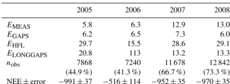
Table B1.Uncertainty analysis of the annual CO₂balance, NEE (g CO2m−2a−1). Error components are explained in the text, and nobs denotes the number of accepted flux observations in 2005– 2008.

2005 2006 2007 2008

E_MEAS 5.8 6.3 12.9 13.0

E_GAPS 6.2 6.5 7.3 6.0

EHFL 29.7 15.5 28.6 29.1

ELONGGAPS 20.8 113 13.2 13.3

n_obs 7868 7240 11 678 12 842

(44.9 %) (41.3 %) (66.7 %) (73.3 %) NEE±error −991±37 −516±114 −952±35 −970±35

Appendix B: Uncertainty analysis of NEE

The uncertainty of the annual CO2 balance was estimated

separately for each year. We followed here the approaches presented by Aurela et al. (2002), Lohila et al. (2011) and Räsänen et al. (2017). The random error arising from the stochastic variability of turbulent fluxes (EMEAS) was

es-timated, similarly to Räsänen et al. (2017), from the dif-ference between the measurements and the corresponding values obtained from the gap-filling model fits (Eqs. A1– A4 in Appendix A). This error varied between 5.8 and 13 g CO2m−2a−1 in 2005–2008 (Table A1). The same

ap-proach was applied to the random error arising from the gap-filling of the data (EGAPS), which ranged from 6.0 to

7.3 g CO2m−2a−1 in 2005–2008 (Table A1). The

uncer-tainty associated with the corrections for the high-frequency flux loss (EHFL)was estimated at 3 % of the annual balance

(Lohila et al., 2011). For the uncertainty due to the gap-filling of the longer (> 2 days) gaps in the flux data (ELONGGAPS),

we adopted a new approach: as the year 2008 had only a few gaps, we simulated the impact of longer gaps in other years by assuming similar data gaps in the time series of 2008 and then ran the gap-filling procedures for these compromised data. For each gap, a cumulative CO2balance was estimated

from two differently gap-filled datasets, i.e. the original and the simulated, and the difference of these was assumed to represent the error. The annual error was calculated by as-suming that the errors obtained this way for separate gaps were independent of each other. For 2006, a similar simula-tion was also run with the data of 2005 and 2007, and the average of the three annual estimates obtained was taken as the total error related to the gap-filling of long gaps. In 2008, there was only one longer (10 day) gap in December. The uncertainty due to this gap was calculated by adopting the daily errors estimated for December 2007, resulting in an ELONGGAPS of 13.3 g CO2m−2a−1for 2008. The total

un-certainty in the annual balance was calculated by assuming thatEMEAS,EGAPSandELONGGAPSare independent.

The total error of±37 g CO2m−2a−1in 2005 was

signif-icantly reduced from that (±100 g m−2a−1)reported by Lo-hila et al. (2011). This was mainly due to the different

ap-proach adopted for the error estimates for the compensation of long data gaps: for this, Lohila et al. (2011) shifted model parameters 2 weeks forward and backward, which resulted in a relative error of 10.7 % of the annual balance. We consider the present approach more realistic, as it is based on assess-ing the effect of realised gaps on actual measurement data. However, it is obvious that the uncertainty estimate for 2006 is limited by the fact that the summer of that year was excep-tionally dry, and the changes in NEE induced by the drought cannot be accurately estimated based on the data of 2008. It is likely that the dynamics of photosynthesis and respiration during a dry summer are different from a normal year. This hypothesis gains support from the observation that theRECO

and GPP parameters in August 2006 differed markedly from those estimated for the other years (Fig. 5).

As a further sensitivity test, we estimated the most conser-vative range for the NEE uncertainty in summer 2006. Be-cause our gap-filling model fills the long gaps by linear in-terpolation, the outcome depends on the selection of the start and end points of the interpolation. The sensitivity test was performed by assuming different parameter scenarios dur-ing the longest gap in the parameters (13 June–4 August, during which there were only 212 valid NEE observations available). In one scenario, a parameter had the starting point value during the whole gap, while in the other it dropped im-mediately to the level at the end point and stayed there over the whole gap. The annual NEE was calculated for each com-bination of differentRREFand GPMAX dynamics. The two

most extreme cases (either bothRREF and GPMAX were

re-duced for the whole gap, or both were increased) prore-duced an annual NEE of−377 and−844 g CO2m−2s−1, respectively.

These can be considered as the most conservative estimates of annual NEE, and thus we can safely conclude that the an-nual NEE was negative in 2006, i.e. the ecosystem acted as a CO2sink even during the exceptionally dry year.

Despite the large gaps during the growing season of 2006, and the large uncertainty resulting from these, the annual NEE balance of 2006 differed significantly from the other years. This difference between two annual balances (NEEi and NEEi+1)was considered significant if the 95 %

confi-dence interval of the difference, defined as (NEEi+1−NEEi)±2

q

Appendix C

Table C1.Parameter values of forest floor CO2efflux models (Eq. 1) for different collar treatments (A=peat, B=peat+litter, C=peat+ litter+roots and D=peat+litter+roots+ground vegetation) and years.RREF5andRREF30are respirations at 10◦C for the 5 and 30 cm depths (g CO2m−2h−1),E05andE030are is temperature sensitivities of respiration for the same layers,r2is coefficient of determination of the model, and n is the number of observations.

Treatment Plot Years R_REF5 E₀₅ R_REF30 E₀₃₀ r2 n

A 1 2005–2006 0.151 302.4 0.088 716.4 0.76 127

A 1 2007–2008 0.124 319.5 0.027 755.2 0.78 108

A 2 2005–2006 0.138 359.7 0.072 754.5 0.77 105

A 2 2007–2008 0.104 431.5 0.021 418.2 0.90 108

A 3 2005–2006 0.127 324.6 0.087 1011.4 0.77 113

A 3 2007–2008 0.120 299.6 0.015 508.6 0.79 107

A 4 2005–2006 0.086 432.6 0.123 297.7 0.62 114

A 4 2007–2008 0.112 331.1 0.027 511.7 0.64 102

B 1 2005–2006 0.175 284.7 0.142 660.2 0.75 135

B 2 2005–2006 0.159 282.6 0.199 560.7 0.72 121

B 3 2005–2006 0.183 244.6 0.146 1053.0 0.67 125

B 4 2005–2006 0.102 303.7 0.183 584.6 0.82 127

C 1 2005–2006 0.237 338.0 0.163 942.3 0.77 145

C 2 2005–2006 0.152 193.3 0.217 532.9 0.49 131

C 3 2005–2006 0.139 311.9 0.228 605.9 0.58 124

C 4 2005–2006 0.204 240.8 0.261 824.9 0.46 137

D 1 2005–2006 0.165 339.3 0.202 741.3 0.50 130

D 1 2007–2008 0.171 360.5 0.146 885.8 0.54 107

D 2 2005–2006 0.192 361.4 0.295 593.3 0.70 129

D 2 2007–2008 0.195 383.2 0.254 518.9 0.71 105

D 3 2005–2006 0.050 581.4 0.319 411.4 0.56 129

D 3 2007–2008 0.123 261.0 0.300 586.8 0.58 106

D 4 2005–2006 0.265 280.4 0.280 1115.6 0.62 121