R E S E A R C H A R T I C L E
Open Access
Estimating the sample mean and standard
deviation from the sample size, median, range
and/or interquartile range
Xiang Wan
1†, Wenqian Wang
2†, Jiming Liu
1and Tiejun Tong
3*Abstract
Background: In systematic reviews and meta-analysis, researchers often pool the results of the sample mean and standard deviation from a set of similar clinical trials. A number of the trials, however, reported the study using the median, the minimum and maximum values, and/or the first and third quartiles. Hence, in order to combine results, one may have to estimate the sample mean and standard deviation for such trials.
Methods: In this paper, we propose to improve the existing literature in several directions. First, we show that the sample standard deviation estimation in Hozo et al.’s method (BMC Med Res Methodol 5:13, 2005) has some serious limitations and is always less satisfactory in practice. Inspired by this, we propose a new estimation method by incorporating the sample size. Second, we systematically study the sample mean and standard deviation estimation problem under several other interesting settings where the interquartile range is also available for the trials.
Results: We demonstrate the performance of the proposed methods through simulation studies for the three frequently encountered scenarios, respectively. For the first two scenarios, our method greatly improves existing methods and provides a nearly unbiased estimate of the true sample standard deviation for normal data and a slightly biased estimate for skewed data. For the third scenario, our method still performs very well for both normal data and skewed data. Furthermore, we compare the estimators of the sample mean and standard deviation under all three scenarios and present some suggestions on which scenario is preferred in real-world applications.
Conclusions: In this paper, we discuss different approximation methods in the estimation of the sample mean and standard deviation and propose some new estimation methods to improve the existing literature. We conclude our work with a summary table (an Excel spread sheet including all formulas) that serves as a comprehensive guidance for performing meta-analysis in different situations.
Keywords: Interquartile range, Median, Meta-analysis, Sample mean, Sample size, Standard deviation
Background
In medical research, it is common to find that several similar trials are conducted to verify the clinical effec-tiveness of a certain treatment. While individual trial study could fail to show a statistically significant treatment effect, systematic reviews and meta-analysis of combined results might reveal the potential benefits of treatment. For instance, Antman et al. [1] pointed out that systematic
*Correspondence: [email protected]
†Equal Contributors
3Department of Mathematics, Hong Kong Baptist University, Kowloon Tong, Hong Kong
Full list of author information is available at the end of the article
reviews and meta-analysis of randomized control trials would have led to earlier recognition of the benefits of thrombolytic therapy for myocardial infarction and may save a large number of patients.
Prior to the 1990s, the traditional approach to com-bining results from multiple trials is to conduct narrative (unsystematic) reviews, which are mainly based on the experience and subjectivity of experts in the area [2]. However, this approach suffers from many critical flaws. The major one is due to inconsistent criteria of different reviewers. To claim a treatment effect, different reviewers may use different thresholds, which often lead to opposite
conclusions from the same study. Hence, from the mid-1980s, systematic reviews and meta-analysis have become an imperative tool in medical effectiveness measurement. Systematic reviews use specific and explicit criteria to identify and assemble related studies and usually pro-vide a quantitative (statistic) estimate of aggregate effect over all the included studies. The methodology in system-atic reviews is usually referred to as meta-analysis. With the combination of several studies and more data taken into consideration in systematic reviews, the accuracy of estimations will get improved and more precise interpre-tations towards the treatment effect can be achieved via meta-analysis.
In meta-analysis of continuous outcomes, the sample size, mean, and standard deviation are required from included studies. This, however, can be difficult because results from different studies are often presented in dif-ferent and non-consistent forms. Specifically in medi-cal research, instead of reporting the sample mean and standard deviation of the trials, some trial studies only report the median, the minimum and maximum val-ues, and/or the first and third quartiles. Therefore, we need to estimate the sample mean and standard devia-tion from these quantities so that we can pool results in a consistent format. Hozo et al. [3] were the first to address this estimation problem. They proposed a simple method for estimating the sample mean and the sample variance (or equivalently the sample standard deviation) from the median, range, and the size of the sample. Their method is now widely accepted in the literature of sys-tematic reviews and meta-analysis. For instance, a search of Google Scholar on November 12, 2014 showed that the article of Hozo et al.’s method has been cited 722 times where 426 citations are made recently in 2013 and 2014.
In this paper, we will show that the estimation of the sample standard deviation in Hozo et al.’s method has some serious limitations. In particular, their estimator did not incorporate the information of the sample size and so consequently, it is always less satisfactory in practice. Inspired by this, we propose a new estimation method that will greatly improve their method. In addition, we will investigate the estimation problem under several other interesting settings where the first and third quartiles are also available for the trials.
Throughout the paper, we define the following summary statistics:
a=the minimum value, q1=the first quartile,
m=the median, q3=the third quartile,
b=the maximum value, n=the sample size.
The{a,q1,m,q3,b}is often referred to as the 5-number summary [4]. Note that the 5-number summary may not always be given in full. The three frequently encountered scenarios are:
C1= {a,m,b;n}, C2= {a,q1,m,q3,b;n}, C3= {q1,m,q3;n}.
Hozo et al.’s method only addressed the estimation of the sample mean and variance under ScenarioC1while Sce-nariosC2 andC3are also common in systematic review and meta-analysis. In Sections ‘Methods’ and ‘Results’, we study the estimation problem under these three scenar-ios, respectively. Simulation studies are conducted in each scenario to demonstrate the superiority of the proposed methods. We conclude the paper in Section ‘Discussion’ with some discussions and a summary table to provide a comprehensive guidance for performing meta-analysis in different situations.
Methods
EstimatingX¯andSfromC1
ScenarioC1assumes that the median, the minimum, the maximum and the sample size are given for a clinical trial study. This is the same assumption as made in Hozo et al.’s method. To estimate the sample mean and standard devia-tion, we first review the Hozo et al.’s method and point out some limitations of their method in estimating the sam-ple standard deviation. We then propose to improve their estimation by incorporating the information of the sample size.
Throughout the paper, we let X1,X2,. . .,Xn be a ran-dom sample of size n from the normal distribution Nμ,σ2, andX
(1) ≤ X(2) ≤ · · · ≤ X(n) be the ordered statistics of X1,X2,· · ·,Xn. Also for the sake of simplic-ity, we assume thatn = 4Q + 1 withQbeing a positive integer. Then
a=X(1) ≤ X(2) ≤ · · · ≤ X(Q+1)=q1
≤ X(Q+2) ≤ · · · ≤ X(2Q+1)=m ≤ X(2Q+2) ≤ · · · ≤ X(3Q+1)=q3
≤ X(3Q+2) ≤ · · · ≤ X(4Q+1)=X(n)=b. (1)
In this section, we are interested in estimating the sam-ple meanX¯ =ni=1Xiand the sample standard deviation
S=ni=1(Xi− ¯X)2/(n−1)
1/2
Hozo et al.’s method
For ease of notation, letM = 2Q+1. Then,M = (n+ 1)/2. To estimate the mean value, Hozo et al. applied the following inequalities:
a ≤ X(1) ≤ a
a ≤ X(i) ≤ m (i=2,. . .,M−1)
m ≤ X(M) ≤ m
m ≤ X(i) ≤ b (i=M+1,. . .,n−1)
b ≤ X(n) ≤ b.
Adding up all above inequalities and dividing byn, we haveLB1≤ ¯X≤UB1, where the lower and upper bounds are
LB1= a+m
2 +
2b−a−m
2n ,
UB1=
m+b
2 +
2a−m−b
2n .
Hozo et al. then estimated the sample mean by
LB1+UB1
2 =
a+2m+b
4 +
a−2m+b
4n . (2)
Note that the second term in (2) is negligible when the sample size is large. A simplified mean estimation is given as
¯
X≈ a+2m+b
4 . (3)
For estimating the sample standard deviation, by assum-ing that the data are non-negative, Hozo et al. applied the following inequalities:
aX(1) ≤ X(21) ≤ aX(1)
aX(i) ≤ X(i)2 ≤ mX(i) (i=2,. . .,M−1)
mX(M) ≤ X(M)2 ≤ mX(M) (4)
mX(i) ≤ X(i)2 ≤ bX(i) (i=M+1,. . .,n−1)
bX(n) ≤ X(n)2 ≤ bX(n).
With some simple algebra and approximations on the formula (4), we haveLSB1≤ni=1Xi2≤USB1, where the lower and upper bounds are
LSB1=a2+m2+b2+(M−2)
a2+am+m2+mb
2 ,
USB1=a2+m2+b2+(M−2)
am+m2+mb+b2
2 .
Then by (3) and the approximationni=1Xi2≈(LSB1+
USB1)/2, the sample standard deviation is estimated by
S=√S2, where
S2= 1
n−1
n
i=1
Xi2−nX¯2
≈ 1
n−1
a2+m2+b2+(n−3)
2
(a+m)2+(m+b)2 4
− n(a+2m+b)2 16
.
Whennis large, it results in the following well-known range rule of thumb:
S≈ b−a
4 . (5)
Note that the range rule of thumb (5) is independent of the sample size. It may not work well in practice, espe-cially when n is extremely small or large. To overcome this problem, Hozo et al. proposed the following improved range rule of thumb with respect to the different size of the sample: S≈ ⎧ ⎪ ⎪ ⎪ ⎪ ⎪ ⎪ ⎪ ⎨ ⎪ ⎪ ⎪ ⎪ ⎪ ⎪ ⎪ ⎩ 1 √ 12
(b−a)2+ (a−2m+b) 2
4
1/2
n≤15
b−a
4 15<n≤70
b−a
6 n>70,
(6)
where the formula forn≤15 is derived under the equidis-tantly spaced data assumption, and the formula forn>70 is suggested by the Chebyshev’s inequality [5]. Note also that when the data are symmetric, we havea+b ≈ 2m and so
1 √
12
(b−a)2+ (a−2m+b)
2
4
1/2
≈ b√−a 12. Hozo et al. showed that the adaptive formula (6) per-forms better than the original formula (5) in most settings.
Improved estimation of S
We think, however, that the adaptive formula (6) may still be less accurate for practical use. First, the threshold val-ues 15 and 70 are suggested somewhat arbitrarily. Second, given the normal dataN(μ,σ2)withσ >0 being a finite value, we know thatσ ≈ (b−a)/6 → ∞ asn → ∞. This contradicts to the assumption thatσis a finite value. Third, the non-negative data assumption in Hozo et al.’s method is also quite restrictive.
In this section, we propose a new estimator to further improve (6) and, in addition, we remove the non-negative assumption on the data. Let Z1,. . .,Zn be independent and identically distributed (i.i.d.) random variables from the standard normal distributionN(0, 1), andZ(1)≤ · · · ≤
Z(n) be the ordered statistics of Z1,. . .,Zn. Then Xi =
μ+σZiandX(i)=μ+σZ(i)fori=1,. . .,n. In particular, we havea=μ+σZ(1)andb=μ+σZ(n). SinceE(Z(1))
lettingξ(n) = 2E(Z(n)), we choose the following estima-tion for the sample standard deviaestima-tion:
S≈ b−a
ξ(n). (7)
Note that ξ(n) plays an important role in the sample standard deviation estimation. If we let ξ(n) ≡ 4, then (7) reduces to the original rule of thumb in (5). If we let
ξ(n)=√12 forn≤15, 4 for 15<n≤70, or 6 forn>70, then (7) reduces to the improved rule of thumb (6).
Next, we present a method to approximate ξ(n) and establish an adaptive rule of thumb for standard devia-tion estimadevia-tion. By David and Nagaraja’s method [6], the expected value ofZ(n)is
E(Z(n))=n
∞
−∞z[(z)]
n−1φ(z)dz,
whereφ(z) = √1 2πe−z
2/2
is the probability density
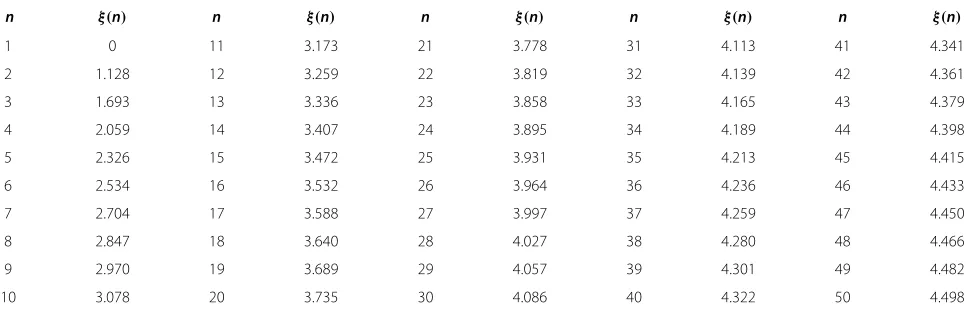
func-tion and(z)=−∞z φ(t)dtis the cumulative distribution function of the standard normal distribution. For ease of reference, we have computed the values ofξ(n)by numer-ical integration using the computer in Table 1 fornup to 50. From Table 1, it is evident that the adaptive formula (6) in Hozo et al.’s method is less accurate and also less flexible.
When n is large (say n > 50), we can apply Blom’s method [7] to approximate E(Z(n)). Specifically, Blom suggested the following approximation for the expected values of the order statistics:
EZ(r)≈−1
r−α
n−2α+1
, r=1,. . .,n, (8) where −1(z) is the inverse function of(z), or equiv-alently, the upperzth percentile of the standard normal distribution. Blom observed that the value ofαincreases asnincreases, with the lowest value being 0.330 forn=2. Overall, Blom suggestedα=0.375 as a compromise value for practical use. Further discussion on the choice of α
can be seen, for example, in [8] and [9]. Finally, by (7) and (8) with r = nandα = 0.375, we estimate the sample standard deviation by
S≈ b−a
2−1n−0.375 n+0.25
. (9)
In the statistical software R, the upper zth percentile
−1(z)can be computed by the command “qnorm(z)”. EstimatingX¯andSfromC2
Scenario C2 assumes that the first quartile, q1, and the third quartile, q3, are also available in addition toC1. In this setting, Bland’s method [10] extended Hozo et al.’s results by incorporating the additional information of the interquartile range (IQR). He further claimed that the new estimators for the sample mean and standard deviation are superior to those in Hozo et al.’s method. In this section, we first review the Bland’s method and point out some limitations of this method. We then, accordingly, propose to improve this method by incorporating the size of a sample.
Bland’s method
Noting thatn = 4Q+1, we have Q = (n−1)/4. To estimate the sample mean, Bland’s method considered the following inequalities:
a ≤ X(1) ≤ a
a ≤ X(i) ≤ q1 (i=2,. . .,Q)
q1 ≤ X(Q+1) ≤ q1
q1 ≤ X(i) ≤ m (i=Q+2,. . ., 2Q)
m ≤X(2Q+1) ≤ m
m ≤ X(i) ≤ q3 (i=2Q+2,. . ., 3Q)
q3 ≤X(3Q+1) ≤ q3
q3 ≤ X(i) ≤ b (i=3Q+2,. . .,n−1)
b ≤ X(n) ≤ b.
Table 1 Values ofξ(n)in the formula (7) and the formula (12) forn≤50
n ξ(n) n ξ(n) n ξ(n) n ξ(n) n ξ(n)
1 0 11 3.173 21 3.778 31 4.113 41 4.341
2 1.128 12 3.259 22 3.819 32 4.139 42 4.361
3 1.693 13 3.336 23 3.858 33 4.165 43 4.379
4 2.059 14 3.407 24 3.895 34 4.189 44 4.398
5 2.326 15 3.472 25 3.931 35 4.213 45 4.415
6 2.534 16 3.532 26 3.964 36 4.236 46 4.433
7 2.704 17 3.588 27 3.997 37 4.259 47 4.450
8 2.847 18 3.640 28 4.027 38 4.280 48 4.466
9 2.970 19 3.689 29 4.057 39 4.301 49 4.482
Adding up all above inequalities and dividing by n, it results inLB2 ≤ ¯X ≤ UB2, where the lower and upper bounds are
LB2= a+q1+m+q3
4 +
4b−a−q1−m−q3
4n ,
UB2=
q1+m+q3+b
4 +
4a−q1−m−q3−b
4n .
Bland then estimated the sample mean by (LB2 +
UB2)/2. When the sample size is large, by ignoring the negligible second terms inLB2andUB2, a simplified mean estimation is given as
¯
X≈ a+2q1+2m+2q3+b
8 . (10)
For the sample standard deviation, Bland considered some similar inequalities as in (4). Then with some sim-ple algebra and approximation, it results in LSB2 ≤ n
i=1Xi2≤USB2, where the lower and upper bounds are
LSB2 = 18
(n+3)a2+q21+m2+q23+8b2 +(n−5)(aq1+q1m+mq3+q3b)
,
USB2 = 18
8a2+(n+3)q12+m2+q23+b2 +(n−5)(aq1+q1m+mq3+q3b)
.
Next, by the approximation ni=1Xi2 ≈ (LSB2 +
USB2)/2,
S2≈ 1
16
a2+2q21+2m2+2q23+b2
+1
8(aq1+q1m+mq3+q3b)− 1
64(a+2q1+2m +2q3+b)2.
(11)
Bland’s method then took the square root√S2to esti-mate the sample standard deviation. Note that the estima-tor (11) is independent of the sample sizen. Hence, it may not be sufficient for general use, especially whennis small
or large. In the next section, we propose an improved esti-mation for the sample standard deviation by incorporating the additional information of the sample size.
Improved estimation of S
Recall that the rangeb−awas used to estimate the sample standard deviation in ScenarioC1. Now for ScenarioC2, since the IQRq3−q1is also known, another approach is to estimate the sample standard deviation by(q3−q1)/η(n), whereη(n) is a function ofn. Taking both methods into account, we propose the following combined estimator for the sample standard deviation:
S≈ 1
2
b−a
ξ(n) +
q3−q1
η(n)
. (12)
Following Section ‘Improved estimation ofS’, we have
ξ(n) =2E(Z(n)). Now we look for an expression forη(n) so that(q3−q1)/η(n)also provides a good estimate ofS. By (1), we haveq1=μ+σZ(Q+1)andq3=μ+σZ(3Q+1). Then,q3−q1=σ
Z(3Q+1)−Z(Q+1). Further, by noting thatEZ(Q+1) = −EZ(3Q+1), we haveE(q3 −q1) = 2σEZ(3Q+1). This suggests that
η(n)=2EZ(3Q+1)
.
In what follows, we propose a method to compute the value ofη(n). By [6], the expected value ofZ(3Q+1)is
EZ(3Q+1)
=((4Q+1)!
Q)!(3Q)!
∞
−∞z[(z)]
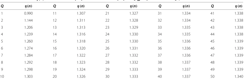
3Q[1−(z)]Qφ(z)dz. In Table 2, we provide the numerical values ofη(n) = 2E(Z(3Q+1))forQ ≤ 50 using the statistical software R. Whennis large, we suggest to apply the formula (8) to approximateη(n). Specifically, noting thatQ=(n−1)/4, we have η(n) ≈ 2−1((0.75n−0.125)/(n+0.25)) for r = 3Q+1 withα = 0.375. Then consequently, for the scenarioC2we estimate the sample standard deviation by
S≈ b−a
4−1n−0.375 n+0.25
+ q3−q1 4−10.75n−0.125
n+0.25
. (13)
Table 2 Values ofη(n)in the formula (12) and the formula (15) forQ≤50, wheren=4Q+1
Q η(n) Q η(n) Q η(n) Q η(n) Q η(n)
1 0.990 11 1.307 21 1.327 31 1.334 41 1.338
2 1.144 12 1.311 22 1.328 32 1.334 42 1.338
3 1.206 13 1.313 23 1.329 33 1.335 43 1.338
4 1.239 14 1.316 24 1.330 34 1.335 44 1.338
5 1.260 15 1.318 25 1.330 35 1.336 45 1.339
6 1.274 16 1.320 26 1.331 36 1.336 46 1.339
7 1.284 17 1.322 27 1.332 37 1.336 47 1.339
8 1.292 18 1.323 28 1.332 38 1.337 48 1.339
9 1.298 19 1.324 29 1.333 39 1.337 49 1.339
We note that the formula (13) is more concise than the formula (11). The numerical comparison between the two formulas will be given in the section of simulation study.
EstimatingX¯andSfromC3
ScenarioC3is an alternative way to report the study other than Scenarios C1 andC2. It reports the first and third quartiles instead of the minimum and maximum values. One main reason to report C3 is because the IQR is usually less sensitive to outliers compared to the range. For the new scenario, we note that Hozo et al.’s method and Bland’s method will no longer be applicable. Partic-ularly, if their ideas are followed, we have the following inequalities:
− ∞ ≤ X(i) ≤ q1 (i=1,. . .,Q)
q1 ≤ X(Q+1) ≤ q1
q1 ≤ X(i) ≤ m (i=Q+2,. . ., 2Q)
m ≤ X(2Q+1) ≤ m
m ≤ X(i) ≤ q3 (i=2Q+2,. . ., 3Q)
q3 ≤ X(3Q+1) ≤ q3
q3 ≤ X(i) ≤ ∞, (i=3Q+2,. . .,n) where the firstQinequalities are unbounded for the lower limit, and the lastQinequalities are unbounded for the upper limit. Now adding up all above inequalities and dividing byn, we have−∞ ≤ ¯X ≤ ∞. This shows that the approaches based on the inequalities do not apply to ScenarioC3.
In contrast, the following procedure is commonly adopted in the recent literature including [11,12]: “If the study provided medians and IQR, we imputed the means and standard deviations as described by Hozo et al. [3]. We calculated the lower and upper ends of the range by multiplying the difference between the median and upper and lower ends of the IQR by 2 and adding or subtracting
the product from the median, respectively”. This
proce-dure, however, performs very poorly in our simulations (not shown).
A quantile method for estimatingX and S¯
In this section, we propose a quantile method for esti-mating the sample mean and the sample standard devia-tion, respectively. In detail, we first revisit the estimation method in ScenarioC2. By (10), we have
¯
X≈ a+2q1+2m+2q3+b
8 =
a+b
8 +
q1+m+q3
4 .
Now for ScenarioC3, aandb are not given. Hence, a reasonable solution is to removeaandb from the esti-mation and keep the second term. By doing so, we have the estimation form as X¯ ≈ (q1 + m+ q3)/C, where
C is a constant. Finally, noting thatE(q1+ m+q3) = 3μ+σEZ(Q+1)+Z2Q+1+Z(3Q+1)
=3μ, we letC=3 and define the estimator of the sample mean as follows:
¯
X≈ q1+m+q3
3 . (14)
For the sample standard deviation, following the idea in constructing (12) we propose the following estimation:
S≈ q3−q1
η(n) , (15) where η(n) = 2EZ(3Q+1)
. As mentioned above that
E(q3 − q1) = 2σEZ(3Q+1)
= ση(n), therefore, the estimator (15) provides a good estimate for the sample standard deviation. The numerical values ofη(n)are given in Table 2 forQ≤50. Whennis large, by the approxima-tionE(Z(3Q+1)) ≈ −1((0.75n−0.125)/(n+0.25)), we can also estimate the sample standard deviation by
S≈ q3−q1
2−10.75n−0.125 n+0.25
. (16)
A similar estimator for estimating the standard devi-ation from IQR is provided in the Cochrane Handbook [13], which is defined as
S≈ q3−q1
1.35 . (17)
Note that the estimator (17) is also independent of the sample sizenand thus may not be sufficient for general use. As we can see from Table 2, the value ofη(n)in the formula (15) converges to about 1.35 whennis large. Note also that the denominator in formula (16) converges to 2∗−1(0.75)which is 1.34898 asntends to infinity. When the sample size is small, our method will provide more accurate estimates than the formula (17) for the standard deviation estimation.
Results
Simulation study forC1
In this section, we conduct simulation studies to com-pare the performance of Hozo et al.’s method and our new method for estimating the sample standard deviation. Fol-lowing Hozo et al.’s settings, we consider five different distributions: the normal distribution with meanμ= 50 and standard deviationσ = 17, the log-normal distribu-tion with locadistribu-tion parameterμ = 4 and scale parameter
σ = 0.3, the beta distribution with shape parameters
20 40 60 80 100
−0.2
−0.1
0.0
0.1
0.2
−0.2
−0.1
0.0
0.1
0.2
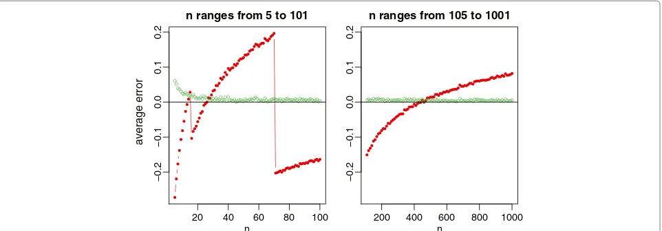
n ranges from 5 to 101 n ranges from 105 to 1001
n
average error
200 400 600 800 1000 n
Figure 1Relative errors of the sample standard deviation estimation for normal data, where the red lines with solid circles represent Hozo et al.’s method, and the green lines with empty circles represent the new method.
maximum values of the sample to estimate the sample standard deviation by the formulas (6) and (9), respec-tively. To assess the accuracy of the two estimates, we define the relative error of each method as
relative error of S= the estimated S−the true S
the true S . (18)
With 1000 simulations, we report the average relative errors in Figure 1 for the normal distribution with the sample size ranging from 5 to 1001, and in Figure 2 for the four non-normal distributions with the sample size ranging from 5 to 101. For normal data which are most commonly assumed in meta-analysis, our new method provides a nearly unbiased estimate of the true sample standard deviation. Whereas for Hozo et al.’s method, we do observe that the best cutoff value is aboutn = 15 for switching between the estimates(b−a)/√12 and(b− a)/4, and is aboutn=70 for switching between(b−a)/4 and(b− a)/6. However, its overall performance is not satisfactory by noting that the estimate always fluctuates from -20% to 20% of the true sample standard deviation. In addition, we note that ξ(27) ≈ 4 from Table 1 and
ξ(n) ≈ 6 when −1((n−0.375)/(n+0.25)) = 3, that is,n = (0.375+0.25∗(3))/(1−(3)) ≈ 463. This coincides with the simulation results in Figure 1 where the method(b−a)/4 crosses thex-axis betweenn= 20 andn =30, and the method(b−a)/6 crosses thex-axis betweenn=400 andn=500.
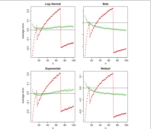
From Figure 2 with the skewed data, our proposed method (9) makes a slightly biased estimate with the rela-tive errors about 5% of the true sample standard deviation. Nevertheless, it is still obvious that the new method is much better compared to Hozo et al.’s method. We also note that, for the beta and Weibull distributions, the best cutoff values ofnshould be larger than 70 for switching between(b−a)/4 and(b−a)/6. This again coincides with
Table one in Hozo et al. [3] where the suggested cutoff value isn=100 for Beta andn=110 for Weibull.
Simulation study forC2
In this section, we evaluate the performance of the pro-posed method (13) and compare it to Bland’s method (11). Following Bland’s settings, we consider (i) the normal dis-tribution with meanμ=5 and standard deviationσ=1, and (ii) the log-normal distribution with location param-eterμ = 5 and scale parameter σ = 0.25, 0.5, and 1, respectively. For simplicity, we consider the sample size beingn=4Q+1, whereQtakes values from 1 to 50. As in Section ‘Simulation study forC1’, we assess the accu-racy of the two estimates by the relative error defined in (18).
20 40 60 80 100
20 40 60 80 100 20 40 60 80 100
20 40 60 80 100
−0.2
−0.1
0.0
0.1
0.2
−0.2
−0.1
0.0
0.1
0.2
Log−Normal
n
average error
−0.2
−0.1
0.0
0.1
Beta
n
Exponential
n
average error
Weibull
n
Figure 2Relative errors of the sample standard deviation estimation for non-normal data (log-normal, beta, exponential and Weibull), where the red lines with solid circles represent Hozo et al.’s method, and the green lines with empty circles represent the new method.
the new method is better than Bland’s method in most settings.
Simulation study forC3
In the third simulation study, we conduct a comparison study that not only assesses the accuracy of the proposed method under ScenarioC3, but also addresses a more real-istic question in meta-analysis, “For a clinical trial study,
which summary statistics should be preferred to report,C1,
C2orC3? and why?"
For the sample mean estimation, we consider the for-mulas (3), (10), and (14) under three different scenarios, respectively. The accuracy of the mean estimation is also assessed by the relative error, which is defined in the same way as that for the sample standard deviation estimation.
Similarly, for the sample standard deviation estimation, we consider the formulas (9), (13), and (15) under three different scenarios, respectively. The distributions we con-sidered are the same as in Section ‘Simulation study for C1’, i.e., the normal, log-normal, beta, exponential and Weibull distributions with the same parameters as those in previous two simulation studies.
0 50 100 150 200
−0.3
−0.2
−
0.1
0.0
0.1
0.2
Normal(5,1)
n
average error
average error
0 50 100 150 200
−0.3
−0.2
−0.1
0.0
0.1
0.2
Log−Normal(5,0.25)
n
0 50 100 150 200
−0.2
0.0
0
.2
0.4
Log−Normal(5,0.5)
n
0 50 100 150 200
−
0.4
−0.2
0.0
0
.2
0.4
0
.6
Log−Normal(5,1)
n
Figure 3Relative errors of the sample standard deviation estimation for normal data and log-normal data, where the red lines with solid circles represent Bland’s method, and the green lines with empty circles represent the new method.
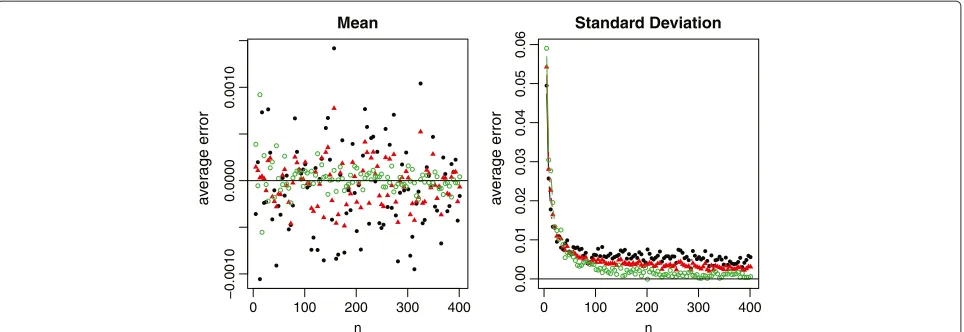
from 1 to 50. With 1000 simulations, we report the aver-age relative errors in Figure 4 for bothX¯ andSwith the normal distribution, in Figure 5 for the sample mean esti-mation with the non-normal distributions, and in Figure 6 for the sample standard deviation estimation with the non-normal distributions.
For normal data which meta-analysis would commonly assume, all three methods provide a nearly unbiased esti-mate of the true sample mean. The relative errors in the sample standard deviation estimation are also very small in most settings (within 1% in general). Among the three methods, however, we recommend to estimateX¯ andS using the summary statistics in Scenario C3. One main reason is because the first and third quartiles are usually
less sensitive to outliers compared to the minimum and maximum values. Consequently,C3produces a more sta-ble estimation thanC1, and alsoC2that is partially affected by the minimum and maximum values.
0 100 200 300 400
−0.0010
0.0000
0.0010
Mean
n
a
v
er
age error
0 100 200 300 400
0.00
0.01
0.02
0.03
0.04
0.05
0.06
Standard Deviation
n
a
v
er
age error
Figure 4Relative errors of the sample mean and standard deviation estimations for normal data, where the black solid circles represent the method under scenarioC1, the red solid triangles represent the method under scenarioC2, and the green empty circles represent the method under scenarioC3.
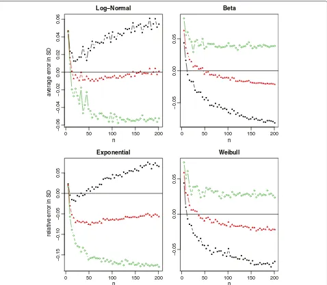
Therefore, we need to be cautious when making the choice betweenC2andC3. It is also noteworthy that (i) the mean estimation from C3 is not sensitive to the sample size, and (ii) C1 and C3 always lead to opposite estimations (one underestimates and the other overestimates the true value). While from Figure 6, we observe that (i) the stan-dard deviation estimation fromC3is quite sensitive to the skewness of the data, (ii)C1andC3would also lead to the opposite estimations except for very small sample sizes, and (iii)C2turns out to be a good compromise for esti-mating the sample standard deviation. Taking both into account, we recommend to report ScenarioC2in clinical trial studies. However, if we do not have all information in the 5-number summary and have to make a decision betweenC1andC3, we recommendC1 for small sample sizes (sayn≤30), andC3for large sample sizes.
Discussion
Researchers often use the sample mean and standard devi-ation to perform meta-analysis from clinical trials. How-ever, sometimes, the reported results may only include the sample size, median, range and/or IQR. To combine these results in meta-analysis, we need to estimate the sample mean and standard deviation from them. In this paper, we first show the limitations of the existing works and then propose some new estimation methods. Here we summa-rize all discussed and proposed estimators under different scenarios in Table 3.
We note that the proposed methods are established under the assumption that the data are normally dis-tributed. In meta-analysis, however, the medians and quartiles are often reported when data do not follow a normal distribution. A natural question arises: “To which extent it makes sense to apply methods that are based on a
normal distribution assumption?” In practice, if the entire
sample or a large part of the sample is known, standard methods in statistics can be applied to estimate the skew-ness or even the density of the population. For the current study, however, the information provided is very limited, say for example, onlya,m,bandnare given in Scenario 1. Under such situations, it may not be feasible to obtain a reliable estimate for the skewness unless we specify the underlying distribution for the population. Note that the underlying distribution is unlikely to be known in prac-tice. Instead, if we arbitrarily choose a distribution (more likely to be misspecified), then the estimates from the wrong model can be even worse than that from the nor-mal distribution assumption. As a compromise, we expect that the proposed formulas under the normal distribution assumption are among the best we can achieve.
Secondly, we note that even if the means and stan-dard deviations can be satisfyingly estimated from the proposed formulas, it still remains a question to which extent it makes sense to use them in a meta-analysis, if the underlying distribution is very asymmetric and one must assume that they don’t represent location and dispersion adequately. Overall, this is a very practical yet challeng-ing question and may warrant more research. In our future research, we propose to develop some test statis-tics (likelihood ratio test, score test, etc) for pre-testing the hypothesis that the distribution is symmetric (or nor-mal) under the scenarios we considered in this article. The result of the pre-test will then suggest us whether or not we should still include the (very) asymmetric data in the meta-analysis. Other proposals that address this issue will also be considered in our future study.
0 50 100 150 200
0.00
0.05
0.10
Log−Normal
n
a
v
er
age error in mean
0 50 100 150 200
−0.03
−
0.02
−0.01
0
.00
0
.01
Beta
n
0 50 100 150 200
−0.2
0.0
0.2
0
.4
0.6
0
.8
Exponential
n
relativ
e error in mean
0 50 100 150 200
−0.05
0
.00
0
.05
0
.10
0
.15
Weibull
n
Figure 5Relative errors of the sample mean estimation for non-normal data (log-normal, beta, exponential and Weibull), where the black lines with solid circles represent the method under scenarioC1, the red lines with solid triangles represent the method under scenarioC2, and the green lines with empty circles represent the method under scenarioC3.
and standard deviation can be applied by simply inputting the sample size, the median, the minimum and maxi-mum values, and/or the first and third quartiles for the appropriate scenario. Furthermore, for ease of compari-son, we have also included Hozo et al.’s method and Bland’s method in the Excel spread sheet.
Conclusions
In this paper, we discuss different approximation meth-ods in the estimation of the sample mean and standard deviation and propose some new estimation methods to improve the existing literature. Through simulation stud-ies, we demonstrate that the proposed methods greatly improve the existing methods and enrich the literature.
0 50 100 150 200
−0.06
−0.04
−
0.02
0.00
0.02
0.04
0.06
Log−Normal
n
a
v
er
age error in SD
0 50 100 150 200
−0.05
0.00
0.05
Beta
n
0 50 100 150 200
−0.15
−0.10
−
0.05
0.00
0.05
Exponential
n
relativ
e error in SD
0 50 100 150 200
−0.05
0.00
0.05
Weibull
n
Figure 6Relative errors of the sample standard deviation estimation for non-normal data (log-normal, beta, exponential and Weibull), where the black lines with solid circles represent the method under scenarioC1, the red lines with solid triangles represent the method under scenarioC2, and the green lines with empty circles represent the method under scenarioC3.
Table 3 Summary table for estimatingX¯ andSunder different scenarios
ScenarioC1 ScenarioC2 ScenarioC3
Hozo et al. (2005) X¯: Eq. (3) – –
S: Eq. (6) – –
Bland (2013) – X¯: Eq. (10) –
– S: Eq. (11) –
New methods X¯: Eq. (3) X¯: Eq. (10) X¯: Eq. (14)
S: Eq. (9) S: Eq. (13) S: Eq. (16)
data assumption in Hozo et al.’s method and so is more applicable in practice.
via two unified quantities, 4−1((n−0.375)/(n+0.25)) and 4−1((0.75n−0.125)/(n+0.25)). With some extra but trivial computing costs, our method makes signifi-cant improvement over Bland’s method when the IQR is available.
Moreover, we pay special attention to an overlooked sce-nario where the minimum and maximum values are not available. We show that the methodology following the ideas in Hozo et al.’s method and Bland’s method will lead to unbounded estimators and is not feasible. On the con-trary, we extend the ideas of our proposed methods in the other two scenarios and again construct a simple but still valid estimator. After that, we take a step forward to compare the estimators of the sample mean and stan-dard deviation under all three scenarios. For simplicity, we have only considered three most commonly used sce-narios, includingC1,C2andC3, in the current article. Our method, however, can be readily generalized to other sce-narios, e.g., when only{a,q1,q3,b;n}are known or when additional quantile information is given.
Additional files
Additional file 1: The plot of each of those distributions in the simulation studies.
Additional file 2: An Excel spread sheet including all formulas.
Competing interests
The authors declare that they have no competing interests.
Authors’ contributions
TT, XW, and JL conceived and designed the methods. TT and WW conducted the implementation and experiments. All authors were involved in the manuscript preparation. All authors read and approved the final manuscript.
Acknowledgements
The authors would like to thank the editor, the associate editor, and two reviewers for their helpful and constructive comments that greatly helped improving the final version of the article. X. Wan’s research was supported by the Hong Kong RGC grant HKBU12202114 and the Hong Kong Baptist University grant FRG2/13-14/005. T.J. Tong’s research was supported by the Hong Kong RGC grant HKBU202711 and the Hong Kong Baptist University grants FRG2/11-12/110, FRG1/13-14/018, and FRG2/13-14/062.
Author details
1Department of Computer Science, Hong Kong Baptist University, Kowloon
Tong, Hong Kong.2Department of Statistics, Northwestern University,
Evanston IL, USA.3Department of Mathematics, Hong Kong Baptist University,
Kowloon Tong, Hong Kong.
Received: 5 September 2014 Accepted: 12 December 2014 Published: 19 December 2014
References
1. Antman EM, Lau J, Kupelnick B, Mosteller F, Chalmers TC:A comparison of results of meta-analyses of randomized control trials and recommendations of clinical experts: treatments for myocardial infarction.J Am Med Assoc1992,268:240–248.
2. Cipriani A, Geddes J:Comparison of systematic and narrative reviews: the example of the atypical antipsychotics.Epidemiol Psichiatr Soc 2003,12:146–153.
3. Hozo SP, Djulbegovic B, Hozo I:Estimating the mean and variance from the median, range, and the size of a sample.BMC Med Res Methodol2005,5:13.
4. Triola M. F:Elementary Statistics, 11th Ed. Addison Wesley; 2009. 5. Hogg RV, Craig AT:Introduction to Mathematical Statistics. Maxwell:
Macmillan Canada; 1995.
6. David HA, Nagaraja HN:Order Statistics, 3rd Ed. Wiley Series in Probability and Statistics; 2003.
7. Blom G:Statistical Estimates and Transformed Beta Variables. New York: John Wiley and Sons, Inc.; 1958.
8. Harter HL:Expected values of normal order statistics.Biometrika1961, 48:151–165.
9. Cramér H:Mathematical Methods of Statistics: Princeton University Press; 1999.
10. Bland M:Estimating mean and standard deviation from the sample size, three quartiles, minimum, and maximum.International Journal of Statistics in Medical Research,in press.2014.
11. Liu T, Li G, Li L, Korantzopoulos P:Association between c-reactive protein and recurrence of atrial fibrillation after successful electrical cardioversion: a meta-analysis.J Am Coll Cardiol2007,49:1642–1648. 12. Zhu A, Ge D, Zhang J, Teng Y, Yuan C, Huang M, Adcock IM, Barnes PJ,
Yao X:Sputum myeloperoxidase in chronic obstructive pulmonary disease.Eur J Med Res2014,19:12.
13. Higgins JPT, Green S:Cochrane Handbook for Systematic Reviews of Interventions: Wiley Online Library; 2008.
doi:10.1186/1471-2288-14-135
Cite this article as:Wanet al.:Estimating the sample mean and standard deviation from the sample size, median, range and/or interquartile range. BMC Medical Research Methodology201414:135.
Submit your next manuscript to BioMed Central and take full advantage of:
• Convenient online submission
• Thorough peer review
• No space constraints or color figure charges
• Immediate publication on acceptance
• Inclusion in PubMed, CAS, Scopus and Google Scholar
• Research which is freely available for redistribution