Abstract: Today’s world is a world of simulation. Now a days,
every product is first designed in virtual domain and then tested for actual implementation. To be able to perform such accurate virtual domain analysis, an accurate mathematical model is needed to be designed in first place. Specifically, in the field of dynamic analysis, so as to continuously monitor the system, the requirement a high-fidelity simulation models in all industries is rising rapidly and this has now become an important part of modern simulation strategies. FEA simulation software’s nowadays could provide very accurate results but they cannot be used directly for dynamic simulations where the environment is continuously changing (input forces, random vibrations etc.). Therefore, this paper deals with design of a mathematical model of a beam to overcome the above stated issue. The technique so used is Model Order Reduction. This method develops an efficient reduced model by reducing the degrees of freedom and also preserving a characteristic behavior of the system. The methodology deals with extracting the mass, and stiffness matrices from FEA simulation software, reducing their size (order), building a second order system using reduced sizes of mass and stiffness, analyzing mode shapes vectors and nodes for input force applications, and generating a state space model of the system.
Index Terms: Finite Element Analysis, Model Order Reduction, Second Order System, State Space.
I. INTRODUCTION
The development of increasing complex structures and mechanical system demand sophisticated to simulation techniques for design control and optimization. Due to complex nature of this system, the size of discrete models resulting from FEA is normally very large. The simulation gets more computationally large and time taken if the full model used.
In the control system design major problem is accurate mathematical modeling of a complicated real system. The mathematical modeling of complicated systems gets higher order differential equation. As per the solving of FEA approach the computational exercise is directly proportional to the cubic of problem size. The computational work minimizes extremely if the size of the problem is minimized. The major goal of modeling and simulation now a day the development of efficient model reduction for creating accurate low order dynamic model.
Normally the experimental results taken from a model test are used to validate and modify a FEM in stage of design and
Revised Manuscript Received on August 05, 2019
Daroga Ajahar M, Mechanical design Engineering, Vishwakarma Institute of Technology, Pune, India.
Dr. M. K. Nalawade, Mechanical design Engineering, Vishwakarma Institute of Technology, Pune, India.
analysis. Due to difficulty of possible structural system and constrained of testing method, the measured data from model is incomplete. This means that incompleteness of measured degree of freedom. The number of measured DOF is excess minimum than that of the total DOF in the FEA model. This problem can be solved by two ways first one is reducing the FEA model to the size of the experimental model and enlarge experimental model to the size of the FEA model. In above both cases we need model order reduction.
Model Order Reduction (MOR) aim is minimize the computational exercise during in time the accuracy of result does not affect it will remain same. Model order reduction replace the large-scale original model by a smaller one by reducing degree of freedom. Control system MOR because minimize order models are very acceptable to design a control system in normal the order of controller increases with the high order of system, and this led to more complex system to design.
Now a day demand of model order reduction increases from all type of analysis, especially in structural analysis because of finite element analysis using everywhere. The working method of finite element is dividing the model in small parts and summation of all small element which leads to approximate to actual system. For more accurate results divide system into very small parts by fine meshing. So fine mesh increases the accuracy of analysis result but same time fine mesh increase the node and element and it goes up to thousand of degree of freedom. These problem-solving increases computational work and time required to solve, which is not good for analysis and optimization as well as controller design. So model order reduction overcome the above stated issue.
II. MODEL&FEA
Modelling a cantilever beam using boundary condition. Doing Modal analysis at both condition free free and fixed condition then solved, taking this results in APDL for extracting mass matrix and stiffness matrix. Important is node connection (i.e. node ordering). Fig 2 showing node number and from this node ordering in APDL [6].
Dimension: 0.376m*0.0262*0.00262m Modulus of elasticity: 6.9e10 N/m2 Density: 2700 kg/m3
Governing equations for cantilever beam:
ω = α2
rad/s. (1)
Where α = 1.875, 4.694, 7.885…...
Mathematical Modelling Of Structures Using
Model Order Reduction Technique
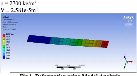
E = 6.9e10 N/m2 ρ = 2700 kg/m3 V = 2.581e-5m3
Fig 1. Deformation using Modal Analysis To know which node fixed and applied force node from APDL required for simulation.
Fig 2. APDL Node Point
Putting α as next mode the frequency calculation it gives only in one direction, but we need in all three direction so calculation of frequency in all direction as
Along Z-axis
I =
(2)
=
3.9267e-11 m4 Along Y-axisI =
(3)=
3.9267e-9 m4 Along X-axisI
=
(4)
=
3.9659e-9 m4For x direction use torsion for calculating frequency. Therefore,
Hz. (5)
III. SECONDORDERSYSTEM&STATESPACE For structural dynamic analyses, governing equations linear second-order differential equations
(6) Where x is co-ordinates
M = Mass matrix K = Stiffness matrix C = Damping matrix F = Forces.
M, C, and K ϵ Rnxn of full order model, DOF of system is n. using Model reduction for the coordinate transformation.
x(t) = T z(t)
T ϵ Rnxm is the co-ordinate transformation matrix and z ϵ Rm is the co-ordinate which is reduce
Now,
(7)
where Mr, Cr, and Kr ϵ Rm x m isthe respective reduced order model of Mass matrix, Damping matrix, Stiffness matrix.
Mr =TTMT, Cr =TTCT, Kr =TTKT, Fr =TTF Now equation is in equilibrium and dynamic equation with reduced form i.e. (m < n), the size of reduced model is very less compare to the actual model without compromise to required frequency range of system.
Considering the governing equation of second order system with state
(8) Y(t)
=
C1z(t) +Du (t) (9)Convert these matrices into the diagonal matrix by Orthogonal property so that only diagonal element present. After that decide the number of modes required for compression.
State Space represent a mathematical model of actual system in control engineering, which contain input, output, state variable and feed forward matrix. Its related to DAE in first order system. State space representation of a linear system with p input, q output and n state variable [3].
(10) Where
y = output x = state vector u = input vector A = State matrix (n*n) B = Input Matrix (n*m) C = Output Matrix (q*n) D = feedforward matrix (q*p)
Therefore,
(11)
So, matrices contained in state space as
A =
B =
C =
D =
From FEA extracted mass matrix and stiffness matrix Mass
Stiff matrix = 1197*1197(free free condition) No. of Node = 412
No. of Element = 42
Convert the motion equation into a state space form and extracted matrix from FEA model in MATLAB will be give the dynamic response of model that one or more inputs with using state space model for active control system.
Note: All mass & stiffness changing but constant is order of DOF.
Using Rayleigh damping calculate damping matrix as
C = αM+βK (12)
ξ = 1/2(α/ω+ β ω) (13)
α = 2ωiωj/ωj2-ωi2 * ξ (14)
β = 2 ξ /ωi+ωj (15)
IV. RESULT
A. Frequency from FEA
[image:3.595.307.542.102.281.2] [image:3.595.54.283.344.535.2]Considering first ten modes shape frequency as only dominant part.
Table 1 showing the frequency for first ten modes
Sr. No Modes Frequency (Hz)
1 1st 15.272
2 2nd 95.689
3 3rd 151.06
4 4th 267.95
5 5th 415.19
6 6th 525.26
7 7th 868.84
8 8th 926.42
9 9th 1248.8
[image:3.595.306.550.356.468.2]10 10th 1299.1
Table 1. FEA Values B. Model Order Reduction
This reading only for ten number of modes we can change as per requirement in table 2.
Sr. No Modes Frequency (Hz)
1 1st 15.25
2 2nd 95.65
3 3rd 150.70
4 4th 267.70
5 5th 415.00
6 6th 524.60
7 7th 869.00
8 8th 921.00
9 9th 1249.0
10 10th 1297.0
Table 2. MOR Values C. Experimental
Setup of cantilever beam placing a strain gauge at fixed end, taking reading on oscilloscope, from time data plot the fft of that data. This reading Cross verification with Impendence Analyzer showing table 3.
Sr. No Modes Frequency (Hz)
1 1st 15.0
2 2nd 94.13
3 3rd 154.36
4 4th 259.14
5 5th 420.00
6 6th 528.00
7 7th 869.58
8 8th 928.32
9 9th 1241.60
10 10th 1297.40
Table 3. Experimental Values
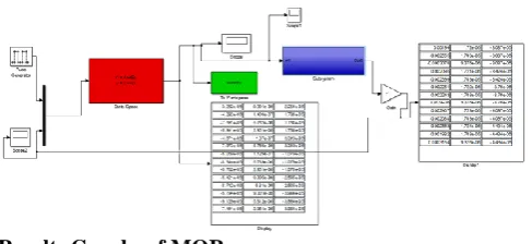
V. MATLABSIMULATIONMOR
Applying force on just one node and one direction it’s gives results shown in graphs regarding frequency.
Results Graphs of MOR
For all direction vibration results showing in below figures. For first ten modes plotting the fft of data gives the frequency response as shown. Amplitude VS Frequency
[image:3.595.303.549.530.678.2]1. Along x-axis vibration
[image:3.595.53.282.582.777.2]Fig 5. Simulation Results along y 3. Along z-axis vibration
[image:4.595.49.292.54.694.2]Fig 6. Simulation Results along z VI. COMPARINGALLRESULTS
Fig 7. All results comparison
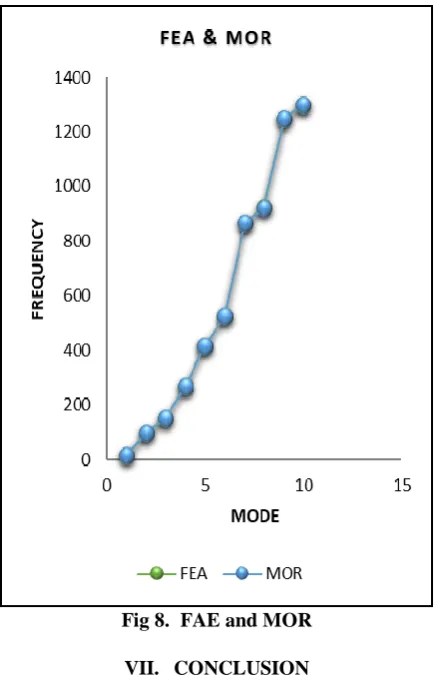
Comparing FEA and MOR aim is to find the error between them so as to future use MOR efficiently, instead of every time FEA we can now using of MOR for dynamic simulation directly. Fig.8 showing the reading of FEA and MOR. Its matching all frequency with minimum error.
Fig 8. FAE and MOR VII. CONCLUSION
In this paper, Comparing theoretical, Finite element analysis and experimental with Model order reduction regarding its frequency output. Error comparing with all results is less than eight percent. Also comparing with full model and reduced model, error is only two percent. So model order reduction this technique allows product designer to more accurately simulate to real time system and to perform dynamic analysisand control vibration.
REFERENCES
1. W. Larbi, J.-F. Deü Reduced order finite element formulations for vibration reduction using piezoelectric shunt damping (2018). 2. Zu-QingQu, Model Order Reduction Techniques with Applications in
Finite Element Analysis (2004).
3. Dr. Dinesh Chandra, Deepika Srivastava, Model Order Reduction of Finite Element Model (2016).
4. Francisco Chinesta, Pierre Ladevèze, Elías Cueto, A Short Review in Model Order Reduction Based on Proper Generalized Decomposition (2017).
5. Mohit Garg, Model Order Reduction and Approximation Analysis for Control System Design (2017).
6. Alain Batailly, How to extract structural matrices (mass, stiffness...) Obtention of elementary cyclic symmetric matrices from an elementary sector in Ansys (2018).
[image:4.595.59.279.339.709.2]Author-3 Photo
AUTHORSPROFILE
Daroga Ajahar M, M. Tech.
Student, Mechanical Design Engineering Vishwakarma Institute of Technology Pune, Email: [email protected], Contact:+919049898300.
Dr. M. K. Nalawade, Ph.D.
Professor, Mechanical Engineering Vishwakarma Institute of Technology Pune, Email: [email protected], Contact: +919822881007