Linear Algebra
Edited by Katrina Glaeser and Travis Scrimshaw First Edition. Davis California, 2013.
This work is licensed under a
Contents
1 What is Linear Algebra? 9
1.1 Organizing Information . . . 9
1.2 What are Vectors? . . . 12
1.3 What are Linear Functions? . . . 15
1.4 So, What is a Matrix? . . . 20
1.4.1 Matrix Multiplication is Composition of Functions . . . 25
1.4.2 The Matrix Detour . . . 26
1.5 Review Problems . . . 30
2 Systems of Linear Equations 37 2.1 Gaussian Elimination . . . 37
2.1.1 Augmented Matrix Notation . . . 37
2.1.2 Equivalence and the Act of Solving . . . 40
2.1.3 Reduced Row Echelon Form . . . 40
2.1.4 Solution Sets and RREF . . . 45
2.2 Review Problems . . . 48
2.3 Elementary Row Operations . . . 52
2.3.1 EROs and Matrices . . . 52
2.3.2 Recording EROs in (M|I) . . . 54
2.3.3 The Three Elementary Matrices . . . 56
2.3.4 LU, LDU, andP LDU Factorizations . . . 58
2.5 Solution Sets for Systems of Linear Equations . . . 63
2.5.1 The Geometry of Solution Sets: Hyperplanes . . . 64
2.5.2 Particular Solution + Homogeneous Solutions . . . 65
2.5.3 Solutions and Linearity . . . 66
2.6 Review Problems . . . 68
3 The Simplex Method 71 3.1 Pablo’s Problem . . . 71
3.2 Graphical Solutions . . . 73
3.3 Dantzig’s Algorithm . . . 75
3.4 Pablo Meets Dantzig . . . 78
3.5 Review Problems . . . 80
4 Vectors in Space, n-Vectors 83 4.1 Addition and Scalar Multiplication in Rn . . . 84
4.2 Hyperplanes . . . 85
4.3 Directions and Magnitudes . . . 88
4.4 Vectors, Lists and Functions: RS . . . . 94
4.5 Review Problems . . . 97
5 Vector Spaces 101 5.1 Examples of Vector Spaces . . . 102
5.1.1 Non-Examples. . . 106
5.2 Other Fields . . . 107
5.3 Review Problems . . . 109
6 Linear Transformations 111 6.1 The Consequence of Linearity . . . 112
6.2 Linear Functions on Hyperplanes . . . 114
6.3 Linear Differential Operators . . . 115
6.4 Bases (Take 1) . . . 115
6.5 Review Problems . . . 118
7 Matrices 121 7.1 Linear Transformations and Matrices . . . 121
7.1.1 Basis Notation . . . 121
7.1.2 From Linear Operators to Matrices . . . 127
5
7.3 Properties of Matrices . . . 133
7.3.1 Associativity and Non-Commutativity . . . 140
7.3.2 Block Matrices . . . 142
7.3.3 The Algebra of Square Matrices . . . 143
7.3.4 Trace . . . 145
7.4 Review Problems . . . 146
7.5 Inverse Matrix . . . 150
7.5.1 Three Properties of the Inverse . . . 150
7.5.2 Finding Inverses (Redux). . . 151
7.5.3 Linear Systems and Inverses . . . 153
7.5.4 Homogeneous Systems . . . 154
7.5.5 Bit Matrices . . . 154
7.6 Review Problems . . . 155
7.7 LU Redux . . . 159
7.7.1 Using LU Decomposition to Solve Linear Systems . . . 160
7.7.2 Finding an LU Decomposition. . . 162
7.7.3 Block LDU Decomposition. . . 165
7.8 Review Problems . . . 166
8 Determinants 169 8.1 The Determinant Formula . . . 169
8.1.1 Simple Examples . . . 169
8.1.2 Permutations . . . 170
8.2 Elementary Matrices and Determinants . . . 174
8.2.1 Row Swap . . . 175
8.2.2 Row Multiplication . . . 176
8.2.3 Row Addition . . . 177
8.2.4 Determinant of Products . . . 179
8.3 Review Problems . . . 182
8.4 Properties of the Determinant . . . 186
8.4.1 Determinant of the Inverse . . . 190
8.4.2 Adjoint of a Matrix . . . 190
8.4.3 Application: Volume of a Parallelepiped . . . 192
8.5 Review Problems . . . 193
9 Subspaces and Spanning Sets 195 9.1 Subspaces . . . 195
9.3 Review Problems . . . 202
10 Linear Independence 203 10.1 Showing Linear Dependence . . . 204
10.2 Showing Linear Independence . . . 207
10.3 From Dependent Independent . . . 209
10.4 Review Problems . . . 210
11 Basis and Dimension 213 11.1 Bases in Rn. . . . 216
11.2 Matrix of a Linear Transformation (Redux) . . . 218
11.3 Review Problems . . . 221
12 Eigenvalues and Eigenvectors 225 12.1 Invariant Directions . . . 227
12.2 The Eigenvalue–Eigenvector Equation. . . 233
12.3 Eigenspaces . . . 236
12.4 Review Problems . . . 238
13 Diagonalization 241 13.1 Diagonalizability . . . 241
13.2 Change of Basis . . . 242
13.3 Changing to a Basis of Eigenvectors . . . 246
13.4 Review Problems . . . 248
14 Orthonormal Bases and Complements 253 14.1 Properties of the Standard Basis . . . 253
14.2 Orthogonal and Orthonormal Bases . . . 255
14.2.1 Orthonormal Bases and Dot Products. . . 256
14.3 Relating Orthonormal Bases . . . 258
14.4 Gram-Schmidt & Orthogonal Complements . . . 261
14.4.1 The Gram-Schmidt Procedure . . . 264
14.5 QR Decomposition . . . 265
14.6 Orthogonal Complements . . . 267
14.7 Review Problems . . . 272
7
16 Kernel, Range, Nullity, Rank 285
16.1 Range . . . 286
16.2 Image . . . 287
16.2.1 One-to-one and Onto . . . 289
16.2.2 Kernel . . . 292
16.3 Summary . . . 297
16.4 Review Problems . . . 299
17 Least squares and Singular Values 303 17.1 Projection Matrices . . . 306
17.2 Singular Value Decomposition . . . 308
17.3 Review Problems . . . 312
A List of Symbols 315 B Fields 317 C Online Resources 319 D Sample First Midterm 321 E Sample Second Midterm 331 F Sample Final Exam 341 G Movie Scripts 367 G.1 What is Linear Algebra? . . . 367
G.2 Systems of Linear Equations . . . 367
G.3 Vectors in Space n-Vectors . . . 377
G.4 Vector Spaces . . . 379
G.5 Linear Transformations . . . 383
G.6 Matrices . . . 385
G.7 Determinants . . . 395
G.8 Subspaces and Spanning Sets . . . 403
G.9 Linear Independence . . . 404
G.10 Basis and Dimension . . . 407
G.11 Eigenvalues and Eigenvectors . . . 409
G.12 Diagonalization . . . 415
G.14 Diagonalizing Symmetric Matrices. . . 428
G.15 Kernel, Range, Nullity, Rank. . . 430
G.16 Least Squares and Singular Values. . . 432
1
What is Linear Algebra?
Many difficult problems can be handled easily once relevant information is organized in a certain way. This text aims to teach you how to organize in-formation in cases where certain mathematical structures are present. Linear algebra is, in general, the study of those structures. Namely
Linear algebra is the study of vectors and linear functions.
In broad terms, vectors are things you can add and linear functions are functions of vectors that respect vector addition. The goal of this text is to teach you to organize information about vector spaces in a way that makes problems involving linear functions of many variables easy. (Or at least tractable.)
To get a feel for the general idea of organizing information, of vectors, and of linear functions this chapter has brief sections on each. We start here in hopes of putting students in the right mindset for the odyssey that follows; the latter chapters cover the same material at a slower pace. Please be prepared to change the way you think about some familiar mathematical objects and keep a pencil and piece of paper handy!
1.1
Organizing Information
Functions of several variables are often presented in one line such as
But lets think carefully; what is the left hand side of this equation doing? Functions and equations are different mathematical objects so why is the equal sign necessary?
A Sophisticated Review of Functions
If someone says
“Consider the function of two variables 7β−13b.”
we do not quite have all the information we need to determine the relationship between inputs and outputs.
Example 1 (Of organizing and reorganizing information)
You own stock in 3 companies: Google,N etf lix, and Apple. The value V of your stock portfolio as a function of the number of shares you own sN, sG, sA of these companies is
24sG+ 80sA+ 35sN.
Here is an ill posed question: what isV 1 2 3
?
The column of three numbers is ambiguous! Is it is meant to denote
• 1 share ofG, 2 shares ofN and 3 shares ofA?
• 1 share ofN, 2 shares ofG and 3 shares ofA?
Do we multiply the first number of the input by 24 or by 35? No one has specified an order for the variables, so we do not know how to calculate an output associated with a particular input.1
A different notation forV can clear this up; we can denoteV itself as an ordered triple of numbers that reminds us what to do to each number from the input.
1Of course we would know how to calculate an output if the input is described in
1.1 Organizing Information 11
DenoteV by 24 80 35 and thus writeV 1 2 3
B
= 24 80 35 1 2 3
to remind us to calculate 24(1) + 80(2) + 35(3) = 334
because we chose the order G A N
and named that order B
so that inputs are interpreted as
sG sA sN
.
If we change the order for the variables we should change the notation for V.
DenoteV by 35 80 24 and thus writeV 1 2 3
B0
= 35 80 24 1 2 3
to remind us to calculate 35(1) + 80(2) + 24(3) = 264.
because we chose the order N A G
and named that order B0
so that inputs are interpreted as
sN sA sG
.
The subscripts B andB0 on the columns of numbers are just symbols2 reminding us
of how to interpret the column of numbers. But the distinction is critical; as shown above V assigns completely different numbers to the same columns of numbers with different subscripts.
There are six different ways to order the three companies. Each way will give different notation for the same function V, and a different way of assigning numbers to columns of three numbers. Thus, it is critical to make clear which ordering is used if the reader is to understand what is written. Doing so is a way of organizing information.
2We were free to choose any symbol to denote these orders. We choseBandB0because
This example is a hint at a much bigger idea central to the text; our choice of order is an example of choosing abasis3.
The main lesson of an introductory linear algebra course is this: you have considerable freedom in how you organize information about certain functions, and you can use that freedom to
1. uncover aspects of functions that don’t change with the choice (Ch12) 2. make calculations maximally easy (Ch 13and Ch 17)
3. approximate functions of several variables (Ch 17).
Unfortunately, because the subject (at least for those learning it) requires seemingly arcane and tedious computations involving large arrays of numbers known as matrices, the key concepts and the wide applicability of linear algebra are easily missed. So we reiterate,
Linear algebra is the study of vectors and linear functions.
In broad terms, vectors are things you can add and linear functions are functions of vectors that respect vector addition.
1.2
What are Vectors?
Here are some examples of things that can be added:
Example 2 (Vector Addition)
(A) Numbers: Both3 and5are numbers and so is 3 + 5.
(B) 3-vectors:
1 1 0
+
0 1 1
=
1 2 1
.
3Please note that this is anexampleof choosing a basis, not a statement of the definition
1.2 What are Vectors? 13
(C) Polynomials: Ifp(x) = 1 +x−2x2+ 3x3 andq(x) =x+ 3x2−3x3+x4 then their sum p(x) +q(x)is the new polynomial 1 + 2x+x2+x4.
(D) Power series: Iff(x) = 1+x+2!1x2+3!1x3+· · · andg(x) = 1−x+2!1x2−3!1x3+· · ·
thenf(x) +g(x) = 1 +2!1x2+4!1x4· · · is also a power series.
(E) Functions: Iff(x) =ex andg(x) = e−x then their sumf(x) +g(x) is the new function2 coshx.
There are clearly different kinds of vectors. Stacks of numbers are not the only things that are vectors, as examples C, D, and E show. Vectors of different kinds can not be added; What possible meaning could the following have?
9 3
+ex
In fact, you should think of all five kinds of vectors above as different kinds, and that you should not add vectors that are not of the same kind. On the other hand, any two things of the same kind “can be added”. This is the reason you should now start thinking of all the above objects as vectors! In Chapter5we will give the precise rules that vector addition must obey. In the above examples, however, notice that the vector addition rule stems from the rules for adding numbers.
When adding the same vector over and over, for example
x+x , x+x+x , x+x+x+x , . . . ,
we will write
2x , 3x , 4x , . . . ,
respectively. For example
4
1 1 0
=
1 1 0
+
1 1 0
+
1 1 0
+
1 1 0
=
4 4 0
.
Defining 4x=x+x+x+x is fine for integer multiples, but does not help us make sense of 1
guess how to multiply a vector by a scalar. For example
1 3
1 1 0
=
1 3 1 3 0
.
A very special vector can be produced from any vector of any kind by scalar multiplying any vector by the number 0. This is called thezero vector
and is usually denoted simply 0. This gives five very different kinds of zero from the 5 different kinds of vectors in examples A-E above.
(A) 0(3) = 0 (The zero number)
(B) 0
1 1 0
=
0 0 0
(The zero 3-vector)
(C) 0 (1 +x−2x2+ 3x3) = 0 (The zero polynomial) (D) 0 1 +x−1
2!x 2+1
3!x
3+· · ·
= 0+0x+0x2+0x3+· · ·(The zero power series) (E) 0 (ex) = 0 (The zero function)
In any given situation that you plan to describe using vectors, you need to decide on a way to add and scalar multiply vectors. In summary:
Vectors are things you can add and scalar multiply.
Examples of kinds of vectors:
• numbers
• n-vectors
• 2nd order polynomials
• polynomials
• power series
1.3 What are Linear Functions? 15
1.3
What are Linear Functions?
In calculus classes, the main subject of investigation was the rates of change of functions. In linear algebra, functions will again be the focus of your attention, but functions of a very special type. In precalculus you were perhaps encouraged to think of a function as a machine f into which one may feed a real number. For each input x this machine outputs a single real number f(x).
In linear algebra, the functions we study will have vectors (of some type) as both inputs and outputs. We just saw that vectors are objects that can be added or scalar multiplied—a very general notion—so the functions we are going to study will look novel at first. So things don’t get too abstract, here are five questions that can be rephrased in terms of functions of vectors. Example 3 (Questions involving Functions of Vectors in Disguise)
(A) What number x satisfies10x= 3?
(B) What 3-vectoru satisfies4
1 1 0
×u=
0 1 1
?
(C) What polynomialp satisfiesR−11p(y)dy= 0 andR−11yp(y)dy= 1?
(D) What power series f(x) satisfiesxdxdf(x)−2f(x) = 0?
(E) What numberx satisfies4x2= 1?
All of these are of the form
(?) What vectorX satisfiesf(X) =B?
with a function5 f known, a vector B known, and a vectorX unknown.
The machine needed for part (A) is as in the picture below.
x 10x
This is just like a function f from calculus that takes in a number x and spits out the number 10x. (You might write f(x) = 10x to indicate this). For part (B), we need something more sophisticated.
x y z
z
−z y−x
,
The inputs and outputs are both 3-vectors. The output is the cross product of the input with... how about you complete this sentence to make sure you understand.
The machine needed for example (C) looks like it has just one input and two outputs; we input a polynomial and get a 2-vector as output.
p
R1
−1p(y)dy
R1
−1yp(y)dy
.
This example is important because it displays an important feature; the inputs for this function are functions.
1.3 What are Linear Functions? 17
While this sounds complicated, linear algebra is the study of simple func-tions of vectors; its time to describe the essential characteristics of linear functions.
Let’s use the letter L to denote an arbitrary linear function and think again about vector addition and scalar multiplication. Also, suppose that v
and u are vectors and c is a number. Since L is a function from vectors to vectors, if we input uintoL, the outputL(u) will also be some sort of vector. The same goes forL(v). (And remember, our input and output vectors might be something other than stacks of numbers!) Because vectors are things that can be added and scalar multiplied, u+v and cu are also vectors, and so they can be used as inputs. The essential characteristic of linear functions is what can be said about L(u+v) and L(cu) in terms of L(u) and L(v).
Before we tell you this essential characteristic, ruminate on this picture.
The “blob” on the left represents all the vectors that you are allowed to input into the functionL, the blob on the right denotes the possible outputs, and the lines tell you which inputs are turned into which outputs.6 A full pictorial description of the functions would require all inputs and outputs 6The domain, codomain, and rule of correspondence of the function are represented by
and lines to be explicitly drawn, but we are being diagrammatic; we only drew four of each.
Now think about adding L(u) andL(v) to get yet another vector L(u) +
L(v) or of multiplyingL(u) bycto obtain the vectorcL(u), and placing both on the right blob of the picture above. But wait! Are you certain that these are possible outputs!?
Here’s the answer
The key to the whole class, from which everything else follows:
1. Additivity:
L(u+v) =L(u) +L(v).
2. Homogeneity:
L(cu) = cL(u).
Most functions of vectors do not obey this requirement.7 At its heart, linear algebra is the study of functions that do.
Notice that the additivity requirement says that the function L respects vector addition: it does not matter if you first add u and v and then input their sum into L, or first input u and v into L separately and then add the outputs. The same holds for scalar multiplication–try writing out the scalar multiplication version of the italicized sentence. When a function of vectors obeys the additivity and homogeneity properties we say that it islinear(this is the “linear” of linear algebra). Together, additivity and homogeneity are calledlinearity. Are there other, equivalent, names for linear functions? yes.
7E.g.: Iff(x) =x2 thenf(1 + 1) = 46=f(1) +f(1) = 2. Try any other function you
1.3 What are Linear Functions? 19
Function = Transformation = Operator
And now for a hint at the power of linear algebra. The questions in examples (A-D) can all be restated as
Lv =w
where v is an unknown, w a known vector, andLis a known linear transfor-mation. To check that this is true, one needs to know the rules for adding vectors (both inputs and outputs) and then check linearity of L. Solving the equation Lv = w often amounts to solving systems of linear equations, the skill you will learn in Chapter 2.
A great example is the derivative operator. Example 4 (The derivative operator is linear)
For any two functions f(x), g(x) and any number c, in calculus you probably learnt that the derivative operator satisfies
1. dxd(cf) =cdxdf,
2. dxd(f +g) = dxdf+ dxdg.
If we view functions as vectors with addition given by addition of functions and with scalar multiplication given by multiplication of functions by constants, then these familiar properties of derivatives are just the linearity property of linear maps.
linear transformation L means that L(u) can be thought of as multiplying the vectoruby the linear operatorL. For example, the linearity ofLimplies that if u, v are vectors and c, dare numbers, then
L
(
cu
+
dv
) =
cLu
+
dLv ,
which feels a lot like the regular rules of algebra for numbers. Notice though, that “uL” makes no sense here.
Remark A sum of multiples of vectors cu +dv is called a linear combination of
uand v.
1.4
So, What is a Matrix?
Matrices are linear functions of a certain kind. They appear almost ubiqui-tously in linear algebra because– and this is the central lesson of introductory linear algebra courses–
Matrices are the result of organizing information related to linear functions.
This idea will take some time to develop, but we provided an elementary example in Section 1.1. A good starting place to learn about matrices is by studyingsystems of linear equations.
1.4 So, What is a Matrix? 21
Each bag contains 2 apples and 4 bananas and each box contains 6 apples and 8 bananas. There are 20 apples and 28 bananas in the room. Find x andy.
The values are the numbers x and y that simultaneously make both of the following equations true:
2x+ 6y = 20
4x+ 8y = 28.
Here we have an example of a System of Linear Equations.8 It’s a collection of equations in which variables are multiplied by constants and summed, and no variables are multiplied together: There are no powers of variables (likex2 or y5), non-integer or negative powers of variables (like y1/7 or x−3), and no places where variables are multiplied together (like xy).
Reading homework: problem 1
Information about the fruity contents of the room can be stored two ways: (i) In terms of the number of apples and bananas.
(ii) In terms of the number of bags and boxes.
Intuitively, knowing the information in one form allows you to figure out the information in the other form. Going from (ii) to (i) is easy: If you knew there were 3 bags and 2 boxes it would be easy to calculate the number of apples and bananas, and doing so would have the feel of multiplication (containers times fruit per container). In the example above we are required to go the other direction, from (i) to (ii). This feels like the opposite of multiplication, i.e., division. Matrix notation will make clear what we are “multiplying” and “dividing” by.
The goal of Chapter 2 is to efficiently solve systems of linear equations. Partly, this is just a matter of finding a better notation, but one that hints at a deeper underlying mathematical structure. For that, we need rules for adding and scalar multiplying 2-vectors;
c
x y
:=
cx cy
and
x y
+
x0 y0
:=
x+x0 y+y0
.
8Perhaps you can see that both lines are of the formLu=vwithu=
x y
an unknown,
Writing our fruity equations as an equality between 2-vectors and then using these rules we have:
2x+ 6y= 20 4x+ 8y= 28
⇐⇒
2x+ 6y
4x+ 8y
= 20 28 ⇐⇒ x 2 4 +y 6 8 = 20 28 .
Now we introduce a function which takes in 2-vectors9and gives out 2-vectors. We denote it by an array of numbers called a matrix .
The function
2 6 4 8
is defined by 2 6 4 8 x y :=x 2 4 +y 6 8 .
A similar definition applies to matrices with different numbers and sizes. Example 6 (A bigger matrix)
1 0 3 4 5 0 3 4
−1 6 2 5
x y z w :=x 1 5 −1 +y
0 0 6 +z
3 3 2 +w
4 4 5 .
Viewed as a machine that inputs and outputs 2-vectors, our 2×2 matrix does the following:
x y
2x+ 6y
4x+ 8y
.
Our fruity problem is now rather concise.
Example 7 (This time in purely mathematical language):
What vector x y satisfies 2 6 4 8 x y = 20 28 ?
9To be clear, we will use the term 2-vector to refer to stacks of two numbers such
as
7 11
. If we wanted to refer to the vectorsx2+ 1 andx3−1 (recall that polynomials
1.4 So, What is a Matrix? 23
This is of the same Lv = w form as our opening examples. The matrix encodes fruit per container. The equation is roughly fruit per container times number of containers equals fruit. To solve for number of containers we want to somehow “divide” by the matrix.
Another way to think about the above example is to remember the rule for multiplying a matrix times a vector. If you have forgotten this, you can actually guess a good rule by making sure the matrix equation is the same as the system of linear equations. This would require that
2 6 4 8
x y
:=
2x+ 6y
4x+ 8y
Indeed this is an example of the general rule that you have probably seen before
p q r s
x y
:=
px+qy rx+sy
=x
p r
+y
q s
.
Notice, that the second way of writing the output on the right hand side of this equation is very useful because it tells us what all possible outputs a matrix times a vector look like – they are just sums of the columns of the matrix multiplied by scalars. The set of all possible outputs of a matrix times a vector is called the column space (it is also the image of the linear function defined by the matrix).
Reading homework: problem 2
Multiplication by a matrix is an example of a Linear Function, because it takes one vector and turns it into another in a “linear” way. Of course, we can have much larger matrices if our system has more variables.
Matrices in Space!
Thus matrices can be viewed as linear functions. The statement of this for the matrix in our fruity example is as follows.
1.
2 6 4 8
λ
x y
=λ
2 6 4 8
x y
2. 2 6 4 8 x y + x0 y0 = 2 6 4 8 x y + 2 6 4 8 x0 y0 .
These equalities can be verified using the rules we introduced so far. Example 8 Verify that
2 6 4 8
is a linear operator.
The matrix-function is homogeneous if the expressions on the left hand side and right hand side of the first equation are indeed equal.
2 6 4 8 λ
a b = 2 6 4 8 λa λb =λa 2 4 +λb 6 8 = 2λa 4λa + 6bc 8bc =
2λa+ 6λb 4λa+ 8λb while λ 2 6 4 8 a b =c a 2 4 +b 6 8 =λ 2a 4a + 6b 8b =λ
2a+ 6b 4a+ 8b
=
2λa+ 6λb 4λa+ 8λb
.
The underlined expressions are identical, so the matrix is homogeneous.
The matrix-function is additive if the left and right side of the second equation are indeed equal. 2 6 4 8 a b + c d = 2 6 4 8
a+c b+d
= (a+c)
2 4
+ (b+d) 6 8 =
2(a+c) 4(a+c)
+
6(b+d) 8(b+d)
=
2a+ 2c+ 6b+ 6d 4a+ 4c+ 8b+ 8d
which we need to compare to
2 6 4 8 a b + 2 6 4 8 c d =a 2 4 +b 6 8 +c 2 4 +d 6 8 = 2a 4a + 6b 8b + 2c 4c + 6d 8d =
2a+ 2c+ 6b+ 6d 4a+ 4c+ 8b+ 8d
.
1.4 So, What is a Matrix? 25
We have come full circle; matrices are just examples of the kinds of linear operators that appear in algebra problems like those in section 1.3. Any equation of the form M v =w with M a matrix, and v, w n-vectors is called a matrix equation. Chapter 2 is about efficiently solving systems of linear equations, or equivalently matrix equations.
1.4.1
Matrix Multiplication is Composition of Functions
What would happen if we placed two of our expensive machines end to end?
?
The output of the first machine would be fed into the second.
x y
2x+ 6y
4x+ 8y
1.(2x+ 6y) + 2.(4x+ 8y)
0.(2x+ 6y) + 1.(4x+ 8y)
=
10x+ 22y
4x+ 8y
Notice that the same final result could be achieved with a single machine:
x y
10x+ 22y
4x+ 8y
.
There is a simple matrix notation for this called matrix multiplication
1 2 0 1
2 6 4 8
=
10 22 4 8
.
Try review problem 6 to learn more about matrix multiplication. In the language10 of functions, if
f :U −→V and g :V −→W
10The notation h:A→B means thathis a function with domainAand codomainB.
the new function obtained by plugging the outputs iff intog is called g◦f,
g◦f :U −→W
where
(g◦f)(u) =g(f(u)).
This is called thecomposition of functions. Matrix multiplication is the tool required for computing the composition of linear functions.
1.4.2
The Matrix Detour
Linear algebra is about linear functions, not matrices. The following presen-tation is meant to get you thinking about this idea constantly throughout the course.
Matrices only get involved in linear algebra when certain notational choices are made.
To exemplify, lets look at the derivative operator again. Example 9 of how matrices come into linear algebra.
Consider the equation
d dx+ 2
f =x+ 1
wheref is unknown (the place where solutions should go) and the linear differential operator dxd + 2is understood to take in quadratic functions (of the formax2+bx+c) and give out other quadratic functions.
Let’s simplify the way we denote the quadratic functions; we will
denote ax2+bx+c as
a
b c
B
.
The subscriptB serves to remind us of our particular notational convention; we will compare to another notational convention later. With the conventionB we can say
d dx+ 2
a b c
B
=
d dx + 2
1.4 So, What is a Matrix? 27
= (2ax+b) + (2ax2+ 2bx+ 2c) = 2ax2+ (2a+ 2b)x+ (b+ 2c)
=
2a 2a+ 2b
b+ 2c B
=
2 0 0 2 2 0 0 1 2
a b c
B
.
That is, our notational convention for quadratic functions has induced a notation for the differential operator dxd + 2as a matrix. We can use this notation to change the way that the following two equations say exactly the same thing.
d dx+ 2
f =x+ 1⇔
2 0 0 2 2 0 0 1 2
a
b c
B
= 0 1 1
B
.
Our notational convention has served as an organizing principle to yield the system of equations
2a = 0 2a+ 2b = 1 b+ 2c = 1
with solution
0 1 2 1 4
B
, where the subscript B is used to remind us that this stack of
numbers encodes the vector 12x+14, which is indeed the solution to our equation since, substituting for f yields the true statement dxd + 2(21x+14) =x+ 1.
It would be nice to have a systematic way to rewrite any linear equation as an equivalent matrix equation. It will be a little while before we can learn to organize information in a way generalizable to all linear equations, but keep this example in mind throughout the course.
A simple example with the knowns (L and V are dxd and 3, respectively) is shown below, although the detour is unnecessary in this case since you know how to anti-differentiate.
1.4 So, What is a Matrix? 29
Example 10 of how a different matrix comes into the same linear algebra problem.
Another possible notational convention is to
denote a+bx+cx2 as
a b c B0 .
With this alternative notation
d dx+ 2
a b c B0 = d dx+ 2
(a+bx+cx2)
= (b+ 2cx) + (2a+ 2bx+ 2cx2) = (2a+b) + (2b+ 2c)x+ 2cx2
=
2a+b 2b+ 2c
2c B0 =
2 1 0 0 2 2 0 0 2
a b c B0 .
Notice that we have obtained a different matrix for the same linear function. The equation we started with
d dx + 2
f =x+ 1⇔
2 1 0 0 2 2 0 0 2
a b c B0 = 1 1 0 B0 ⇔
2a+b= 1 2b+ 2c= 1 2c= 0
has the solution
1 4 1 2 0
. Notice that we have obtained a different 3-vector for the same vector, since in the notational conventionB0 this 3-vector represents 14 +12x.
1.5
Review Problems
You probably have already noticed that understanding sets, functions and basic logical operations is a must to do well in linear algebra. Brush up on these skills by trying these background webwork problems:
Logic 1
Sets 2
Functions 3
Equivalence Relations 4
Proofs 5
Each chapter also has reading and skills WeBWorK problems: Webwork: Reading problems 1 ,2
Probably you will spend most of your time on the following review questions: 1. Problems A, B, and C of example3can all be written asLv =wwhere
L:V −→W ,
(read this asLmaps the set of vectorsV to the set of vectorsW). For each case write down the sets V and W where the vectors v and w
come from.
1.5 Review Problems 31
Remember that the cross productof two 3-vectors is given by
x y z
×
x0 y0 z0
:=
yz0−zy0 zx0−xz0 xy0−yx0
.
Indeed, 3-vectors are special, usually vectors an only be added, not multiplied.
Lets find the forceF (a vector) one must apply to a wrench lying along the vector r =
1 1 0
ft, to produce a torque
0 0 1
ft lb:
(a) Find a solution by writing out this equation with F =
a b c
. (Hint: Guess and check that a solution with a= 0 exists).
(b) Add
1 1 0
to your solution and check that the result is a solution. (c) Give a physics explanation of why there can be two solutions, and
argue that there are, in fact, infinitely many solutions.
(d) Set up a system of three linear equations with the three compo-nents of F as the variables which describes this situation. What happens if you try to solve these equations by substitution? 3. The function P(t) gives gas prices (in units of dollars per gallon) as a
function oftthe year (in A.D. or C.E.), andg(t) is the gas consumption rate measured in gallons per year by a driver as a function of their age. The function g is certainly different for different people. Assuming a lifetime is 100 years, what function gives the total amount spent on gas during the lifetime of an individual born in an arbitrary year t? Is the operator that maps g to this function linear?
4. The differential equation (DE)
d
says that the rate of change of f is proportional to f. It describes exponential growth because the exponential function
f(t) = f(0)e2t
satisfies the DE for any numberf(0). The number 2 in the DE is called the constant of proportionality. A similar DE
d dtf =
2
tf
has a time-dependent “constant of proportionality”.
(a) Do you think that the second DE describes exponential growth? (b) Write both DEs in the form Df = 0 with D a linear operator. 5. Pablo is a nutritionist who knows that oranges always have twice as
much sugar as apples. When considering the sugar intake of schoolchil-dren eating a barrel of fruit, he represents the barrel like so:
sugar fruit
(s, f)
Finda linear operator relating Pablo’s representation to the “everyday” representation in terms of the number of apples and number of oranges. Write your answer as a matrix.
Hint: Letλ represent the amount of sugar in each apple.
1.5 Review Problems 33
6. Matrix Multiplication: LetM and N be matrices
M =
a b c d
and N =
e f g h
,
and v the vector
v =
x y
.
If we first apply N and then M tov we obtain the vector M N v.
(a) Show that the composition of matricesM N is also a linear oper-ator.
(b) Write out the components of the matrix productM N in terms of the components of M and the components of N. Hint: use the
general rule for multiplying a 2-vector by a 2×2 matrix.
(c) Try to answer the following common question, “Is there any sense in which these rules for matrix multiplication are unavoidable, or are they just a notation that could be replaced by some other notation?”
(d) Generalize your multiplication rule to 3×3 matrices.
7. Diagonal matrices: A matrixM can be thought of as an array of num-bersmi
j, known as matrix entries, or matrix components, whereiandj index row and column numbers, respectively. Let
M =
1 2 3 4
= mij.
Compute m1
1, m12, m21 and m22. The matrix entries mi
i whose row and column numbers are the same are called the diagonal of M. Matrix entries mi
j with i 6= j are called
off-diagonal. How many diagonal entries does an n×n matrix have? How many off-diagonal entries does an n×n matrix have?
If all the off-diagonal entries of a matrix vanish, we say that the matrix is diagonal. Let
D=
λ 0 0 µ
and D0 =
λ0 0 0 µ0
Are these matrices diagonal and why? Use the rule you found in prob-lem 6 to compute the matrix products DD0 and D0D. What do you observe? Do you think the same property holds for arbitrary matrices? What about products where only one of the matrices is diagonal?
(p.s. Diagonal matrices play a special role in in the study of matrices in linear algebra. Keep an eye out for this special role.)
8. Find the linear operator that takes in vectors from n-space and gives out vectors from n-space in such a way that
(a) whatever you put in, you get exactly the same thing out as what you put in. Show that it is unique. Can you write this operator as a matrix?
(b) whatever you put in, you get exactly the same thing out as when you put something else in. Show that it is unique. Can you write this operator as a matrix?
Hint: To show something is unique, it is usually best to begin by pre-tending that it isn’t, and then showing that this leads to a nonsensical conclusion. In mathspeak–proof by contradiction.
9. Consider the set S = {∗, ?,#}. It contains just 3 elements, and has no ordering; {∗, ?,#} = {#, ?,∗} etc. (In fact the same is true for {1,2,3} = {2,3,1} etc, although we could make this an ordered set
using 3>2>1.)
(i) Invent a function with domain {∗, ?,#} and codomain R. (Re-member that the domain of a function is the set of all its allowed inputs and the codomain (or target space) is the set where the outputs can live. A function is specified by assigning exactly one codomain element to each element of the domain.)
(ii) Choose an ordering on {∗, ?,#}, and then use it to write your function from part (i) as a triple of numbers.
1.5 Review Problems 35
2
Systems of Linear Equations
2.1
Gaussian Elimination
Systems of linear equations can be written as matrix equations. Now you will learn an efficient algorithm for (maximally) simplifying a system of linear equations (or a matrix equation) – Gaussian elimination.
2.1.1
Augmented Matrix Notation
Efficiency demands a new notation, called an augmented matrix, which we introduce via examples:
The linear system
x + y = 27 2x− y = 0,
is denoted by the augmented matrix
1 1 27 2 −1 0
.
This notation is simpler than the matrix one,
1 1 2 −1
x y
=
27
0
,
Augmented Matrix Notation
Another interesting rewriting is
x 1 2 +y 1 −1 = 27 0 .
This tells us that we are trying to find the combination of the vectors 1 2 and 1 −1
adds up to
27 0
; the answer is “clearly” 9 1 2 + 18 1 −1 .
Here is a larger example. The system
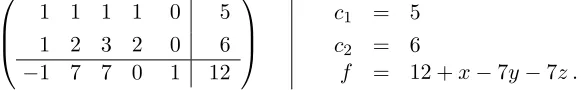
1x+ 3y+ 2z+ 0w = 9 6x+ 2y+ 0z−2w = 0 −1x+ 0y+ 1z+ 1w = 3,
is denoted by the augmented matrix
1 3 2 0 9 6 2 0 −2 0 −1 0 1 1 3
,
which is equivalent to the matrix equation
1 3 2 0 6 2 0 −2 −1 0 1 1
x y z w = 9 0 3 .
Again, we are trying to find which combination of the columns of the matrix adds up to the vector on the right hand side.
For the the general case of r linear equations ink unknowns, the number of equations is the number of rows r in the augmented matrix, and the number of columns k in the matrix left of the vertical line is the number of unknowns, giving an augmented matrix of the form
a1
1 a12 · · · a1k b1
a2
1 a22 · · · a2k b2 ..
. ... ... ...
ar1 ar2 · · · ark br
2.1 Gaussian Elimination 39
Entries left of the divide carry two indices; subscripts denote column number and superscripts row number. We emphasize, the superscripts here do not
denote exponents. Make sure you can write out the system of equations and the associated matrix equation for any augmented matrix.
Reading homework: problem 1
We now have three ways of writing the same question. Let’s put them side by side as we solve the system by strategically adding and subtracting equations. We will not tell you the motivation for this particular series of steps yet, but let you develop some intuition first.
Example 11 (How matrix equations and augmented matrices change in elimination)
x + y = 27 2x − y = 0
⇔
1 1 2 −1
x y = 27 0 ⇔
1 1 27 2 −1 0
.
With the first equation replaced by the sum of the two equations this becomes
3x + 0 = 27 2x − y = 0
⇔
3 0 2 −1
x y = 27 0 ⇔
3 0 27 2 −1 0
.
Let the new first equation be the old first equation divided by 3:
x + 0 = 9
2x − y = 0
⇔
1 0 2 −1
x y = 9 0 ⇔
1 0 9 2 −1 0
.
Replace the second equation by the second equation minus two times the first equation:
x + 0 = 9
0 − y = −18
⇔
1 0 0 −1
x y = 9 −18 ⇔
1 0 9
0 −1 −18
.
Let the new second equation be the old second equation divided by -1:
x + 0 = 9
0 + y = 18 ⇔ 1 0 0 1 x y = 9 18 ⇔
1 0 9 0 1 18
.
Did you see what the strategy was? To eliminate y from the first equation and then eliminate x from the second. The result was the solution to the system.
2.1.2
Equivalence and the Act of Solving
We now introduce the symbol∼which is called “tilde” but should be read as “is (row) equivalent to” because at each step the augmented matrix changes by an operation on its rows but its solutions do not. For example, we found above that
1 1 27 2 −1 0
∼
1 0 9 2 −1 0
∼
1 0 9 0 1 18
.
The last of these augmented matrices is our favorite!
Equivalence Example
Setting up a string of equivalences like this is a means of solving a system of linear equations. This is the main idea of section2.1.3. This next example hints at the main trick:
Example 12 (Using Gaussian elimination to solve a system of linear equations)
x+ y = 5 x+ 2y = 8
⇔
1 1 5 1 2 8
∼
1 1 5 0 1 3
∼
1 0 2 0 1 3
⇔
x+ 0 = 2 0 +y = 3
Note that in going from the first to second augmented matrix, we used the top left1
to make the bottom left entry zero. For this reason we call the top left entry a pivot. Similarly, to get from the second to third augmented matrix, the bottom right entry (before the divide) was used to make the top right one vanish; so the bottom right entry is also called a pivot.
This name pivot is used to indicate the matrix entry used to “zero out” the other entries in its column; the pivot is the number used to eliminate another number in its column.
2.1.3
Reduced Row Echelon Form
For a system of two linear equations, the goal of Gaussian elimination is to convert the part of the augmented matrix left of the dividing line into the matrix
I =
1 0 0 1
2.1 Gaussian Elimination 41
called the Identity Matrix, since this would give the simple statement of a solution x = a, y = b. The same goes for larger systems of equations for which the identity matrix I has 1’s along its diagonal and all off-diagonal entries vanish:
I =
1 0 · · · 0
0 1 0
..
. . .. ... 0 0 · · · 1
Reading homework: problem 2
For many systems, it is not possible to reach the identity in the augmented matrix via Gaussian elimination. In any case, a certain version of the matrix that has the maximum number of components eliminated is said to be the Row Reduced Echelon Form (RREF).
Example 13 (Redundant equations)
x + y = 2
2x + 2y = 4 )
⇔ 1 1 2
2 2 4 !
∼ 1 1 2
0 0 0 !
⇔
(
x + y = 2 0 + 0 = 0
This example demonstrates if one equation is a multiple of the other the identity matrix can not be a reached. This is because the first step in elimination will make the second row a row of zeros. Notice that solutions still exists (1,1) is a solution. The last augmented matrix here is in RREF; no more than two components can be eliminated.
Example 14 (Inconsistent equations)
x + y = 2
2x + 2y = 5 )
⇔ 1 1 2
2 2 5 !
∼ 1 1 2
0 0 1 !
⇔
(
x + y = 2 0 + 0 = 1
This system of equation has a solution if there exists two numbers x, andysuch that
Example 15 (Silly order of equations) A robot might make this mistake:
0x + y = −2
x + y = 7
)
⇔ 0 1 −2
1 1 7 !
∼ · · ·,
and then give up because the the upper left slot can not function as a pivot since the 0 that lives there can not be used to eliminate the zero below it. Of course, the right thing to do is to change the order of the equations before starting
x + y = 7
0x + y = −2 )
⇔ 1 1 7
0 1 −2 !
∼ 1 0 9
0 1 −2 !
⇔
(
x + 0 = 9
0 + y = −2.
The third augmented matrix above is the RREF of the first and second. That is to say, you can swap rows on your way to RREF.
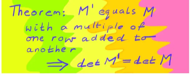
For larger systems of equations redundancy and inconsistency are the ob-structions to obtaining the identity matrix, and hence to a simple statement of a solution in the form x = a, y = b, . . . . What can we do to maximally simplify a system of equations in general? We need to perform operations that simplify our systemwithout changing its solutions. Because, exchanging the order of equations, multiplying one equation by a non-zero constant or adding equations does not change the system’s solutions, we are lead to three operations:
• (Row Swap) Exchange any two rows.
• (Scalar Multiplication) Multiply any row by a non-zero constant.
• (Row Addition) Add one row to another row.
These are called Elementary Row Operations, or EROs for short, and are studied in detail in section 2.3. Suppose now we have a general augmented matrix for which the first entry in the first row does not vanish. Then, using just the three EROs, we could1 then perform the following.
1This is a “brute force” algorithm; there will often be more efficient ways to get to
2.1 Gaussian Elimination 43
Algorithm For Obtaining RREF:
• Make the leftmost nonzero entry in the top row 1 by multiplication.
• Then use that 1 as a pivot to eliminate everything below it.
• Then go to the next row and make the leftmost nonzero entry 1.
• Use that 1 as a pivot to eliminate everything below and above it!
• Go to the next row and make the leftmost nonzero entry 1... etc
In the case that the first entry of the first row is zero, we may first interchange the first row with another row whose first entry is non-vanishing and then perform the above algorithm. If the entire first column vanishes, we may still apply the algorithm on the remaining columns.
Here is a video (with special effects!) of a hand performing the algorithm by hand. When it is done, you should try doing what it does.
Beginner Elimination
This algorithm and its variations is known as Gaussian elimination. The endpoint of the algorithm is an augmented matrix of the form
1 ∗ 0 ∗ 0 · · · 0 ∗ b1 0 0 1 ∗ 0 · · · 0 ∗ b2 0 0 0 0 1 · · · 0 ∗ b3
..
. ... ... ... ... ... 0 0 0 0 0 · · · 1 ∗ bk 0 0 0 0 0 · · · 0 0 bk+1
..
. ... ... ... ... ... ... ... 0 0 0 0 0 · · · 0 0 br
.
This is called Reduced Row Echelon Form (RREF). The asterisks denote the possibility of arbitrary numbers (e.g., the second 1 in the top line of example 13).
The following properties define RREF:
1. In every row the left most non-zero entry is 1 (and is called a pivot). 2. The pivot of any given row is always to the right of the pivot of the
row above it.
3. The pivot is the only non-zero entry in its column. Example 16 (Augmented matrix in RREF)
1 0 7 0 0 1 3 0 0 0 0 1 0 0 0 0
Example 17 (Augmented matrix NOT in RREF)
1 0 3 0 0 0 2 0 0 1 0 1 0 0 0 1
Actually, this NON-example breaks all three of the rules!
The reason we need the asterisks in the general form of RREF is that not every column need have a pivot, as demonstrated in examples13and16. Here is an example where multiple columns have no pivot:
Example 18 (Consecutive columns with no pivot in RREF)
x + y + z + 0w = 2
2x + 2y + 2z + 2w = 4
⇔
1 1 1 0 2 2 2 2 1 4
∼
1 1 1 0 2 0 0 0 1 0
⇔
x + y + z = 2
w = 0.
Note that there was no hope of reaching the identity matrix, because of the shape of the augmented matrix we started with.
2.1 Gaussian Elimination 45
Advanced Elimination
It is important that you are able to convert RREF back into a system of equations. The first thing you might notice is that if any of the numbers
bk+1, . . . , br in2.1.3are non-zero then the system of equations is inconsistent and has no solutions. Our next task is to extract all possible solutions from an RREF augmented matrix.
2.1.4
Solution Sets and RREF
RREF is a maximally simplified version of the original system of equations in the following sense:
• As many coefficients of the variables as possible are 0.
• As many coefficients of the variables as possible are 1.
It is easier to read off solutions from the maximally simplified equations than from the original equations, even when there are infinitely many solutions. Example 19 (Standard approach from a system of equations to the solution set)
x + y + 5w = 1
y + 2w = 6
z + 4w = 8 ⇔
1 1 0 5 1 0 1 0 2 6 0 0 1 4 8
∼
1 0 0 3 −5 0 1 0 2 6 0 0 1 4 8
⇔
x + 3w = −5
y + 2w = 6
z + 4w = 8 ⇔
x = −5 − 3w
y = 6 − 2w
z = 8 − 4w
w = w
⇔ x y z w = −5 6 8 0 +w −3 −2 −4 1 .
There is one solution for each value of w, so the solution set is
−5 6 8 0 +α −3 −2 −4 1
:α∈R
Here is a verbal description of the preceeding example of the standard ap-proach. We say that x, y, and z are pivot variables because they appeared with a pivot coefficient in RREF. Since w never appears with a pivot co-efficient, it is not a pivot variable. In the second line we put all the pivot variables on one side and all the non-pivot variables on the other side and added the trivial equationw=wto obtain a system that allowed us to easily read off solutions.
The Standard Approach To Solution Sets
1. Write the augmented matrix.
2. Perform EROs to reach RREF.
3. Express the pivot variables in terms of the non-pivot variables.
There are always exactly enough non-pivot variables to index your solutions. In any approach, the variables which are not expressed in terms of the other variables are calledfree variables. The standard approach is to use the non-pivot variables as free variables.
Non-standard approach: solve forw in terms ofz and substitute into the other equations. You now have an expression for each component in terms of z. But why pickz instead of y or x? (or x+y?) The standard approach not only feels natural, but is canonical, meaning that everyone will get the same RREF and hence choose the same variables to be free. However, it is important to remember that so long as theirsetof solutions is the same, any two choices of free variables is fine. (You might think of this as the difference between using Google MapsTM or MapquestTM; although their maps may look different, the place hhome sici they are describing is the same!)
When you see an RREF augmented matrix with two columns that have no pivot, you know there will be two free variables.
2.1 Gaussian Elimination 47
1 0 7 0 4 0 1 3 4 1 0 0 0 0 0 0 0 0 0 0
⇔
x + 7z = 4
y+ 3z+4w = 1 ⇔
x = 4 − 7z
y = 1 − 3z − 4w
z = z
w = w
⇔ x y z w = 4 1 0 0 +z −7 −3 1 0 +w 0 −4 0 1
so the solution set is
4 1 0 0 +z −7 −3 1 0 +w 0 −4 0 1
:z, w∈R
.
From RREF to a Solution Set
You can imagine having three, four, or fifty-six non-pivot columns and the same number of free variables indexing your solutions set. In general a solution set to a system of equations with n free variables will be of the form
{xP +µ
1xH1 +µ2xH2 +· · ·+µnxHn :µ1, . . . , µn ∈R}.
The parts of these solutions play special roles in the associated matrix equation. This will come up again and again long after we complete this discussion of basic calculation methods, so we will use the general language of linear algebra to give names to these parts now.
Definition: A homogeneous solution to a linear equation Lx = v, with
L and v known is a vector xH such thatLxH = 0 where 0 is the zero vector.
Particular and Homogeneous Solutions
Check now that the parts of the solutions with free variables as coefficients from the previous examples are homogeneous solutions, and that by adding a homogeneous solution to a particular solution one obtains a solution to the matrix equation. This will come up over and over again. As an example without matrices, consider the differential equation dxd22f = 3. A particular
solution is 32x2 whilex and 1 are homogeneous solutions. The solution set is {3
2x
2+ax+c1 : a, b∈
R}. You can imagine similar differential equations
with more homogeneous solutions.
You need to become very adept at reading off solutions sets of linear systems from the RREF of their augmented matrix; it is a basic skill for linear algebra, and we will continue using it up to the last page of the book!
Worked examples of Gaussian elimination
2.2
Review Problems
Webwork:
Reading problems 1 , 2
Augmented matrix 6
2×2 systems 7, 8, 9, 10, 11, 12
3×2 systems 13, 14
3×3 systems 15, 16, 17
1. State whether the following augmented matrices are in RREF and com-pute their solution sets.
1 0 0 0 3 1 0 1 0 0 1 2 0 0 1 0 1 3 0 0 0 1 2 0
,
1 1 0 1 0 1 0 0 0 1 2 0 2 0 0 0 0 0 1 3 0 0 0 0 0 0 0 0
2.2 Review Problems 49
1 1 0 1 0 1 0 1 0 0 1 2 0 2 0 −1 0 0 0 0 1 3 0 1 0 0 0 0 0 2 0 −2 0 0 0 0 0 0 1 1
.
2. Solve the following linear system:
2x1+ 5x2 −8x3+ 2x4+ 2x5= 0 6x1+ 2x2−10x3+ 6x4+ 8x5= 6 3x1+ 6x2 + 2x3+ 3x4+ 5x5= 6 3x1+ 1x2 −5x3+ 3x4+ 4x5= 3 6x1+ 7x2 −3x3+ 6x4+ 9x5= 9
Be sure to set your work out carefully with equivalence signs∼between each step, labeled by the row operations you performed.
3. Check that the following two matrices are row-equivalent:
1 4 7 10 2 9 6 0
and
0 −1 8 20 4 18 12 0
.
Now remove the third column from each matrix, and show that the resulting two matrices (shown below) are row-equivalent:
1 4 10 2 9 0
and
0 −1 20 4 18 0
.
Now remove the fourth column from each of the original two matri-ces, and show that the resulting two matrimatri-ces, viewed as augmented matrices (shown below) are row-equivalent:
1 4 7 2 9 6
and
0 −1 8 4 18 12
.
Explain why row-equivalence is never affected by removing columns. 4. Check that the system of equations corresponding to the augmented
matrix
1 4 10 3 13 9 4 17 20
has no solutions. If you remove one of the rows of this matrix, does the new matrix have any solutions? In general, can row equivalence be affected by removing rows? Explain why or why not.
5. Explain why the linear system has no solutions:
1 0 3 1 0 1 2 4 0 0 0 6
For which values of k does the system below have a solution?
x − 3y = 6
x + 3z = −3 2x + ky + (3−k)z = 1
Hint
6. Show that the RREF of a matrix is unique. (Hint: Consider what happens if the same augmented matrix had two different RREFs. Try to see what happens if you removed columns from these two RREF augmented matrices.)
7. Another method for solving linear systems is to use row operations to bring the augmented matrix to Row Echelon Form (REF as opposed to RREF). In REF, the pivots are not necessarily set to one, and we only require that all entries left of the pivots are zero, not necessarily entries above a pivot. Provide a counterexample to show that row echelon form is not unique.
Once a system is in row echelon form, it can be solved by “back substi-tution.” Write the following row echelon matrix as a system of equa-tions, then solve the system using back-substitution.
2 3 1 6 0 1 1 2 0 0 3 3
2.2 Review Problems 51
8. Show that this pair of augmented matrices are row equivalent, assuming
ad−bc6= 0:
a b e c d f
!
∼ 1 0
de−bf ad−bc 0 1 afad−−cebc
!
9. Consider the augmented matrix:
2 −1 3 −6 3 1
.
Give a geometric reason why the associated system of equations has no solution. (Hint, plot the three vectors given by the columns of this augmented matrix in the plane.) Given a general augmented matrix
a b e c d f
,
can you find a condition on the numbers a, b, cand d that corresponds to the geometric condition you found?
10. A relation ∼ on a set of objects U is an equivalence relation if the following three properties are satisfied:
• Reflexive: For any x∈U, we have x∼x.
• Symmetric: For any x, y ∈U, if x∼y then y∼x.
• Transitive: For anyx, y andz ∈U, ifx∼yandy∼z thenx∼z. Show that row equivalence of matrices is an example of an equivalence relation.
(For a discussion of equivalence relations, seeHomework 0, Problem 4)
Hint
11. Equivalence of augmented matrices does not come from equality of their solution sets. Rather, we define two matrices to be equivalent if one can be obtained from the other by elementary row operations.
2.3
Elementary Row Operations
Elementary row operations are systems of linear equations relating the old and new rows in Gaussian elimination:
Example 21 (Keeping track of EROs with equations between rows) We refer to the new kth row asRk0 and the oldkth row asRk.
0 1 1 7 2 0 0 4 0 0 1 4
R01=0R1+ R2+0R3
R02= R1+0R2+0R3
R03=0R1+0R2+ R3
∼
2 0 0 4 0 1 1 7 0 0 1 4
R01 R02 R03
=
0 1 0 1 0 0 0 0 1
R1 R2 R3 R0
1=12R1+0R2+0R3
R02=0R1+ R2+0R3
R03=0R1+0R2+ R3
∼
1 0 0 2 0 1 1 7 0 0 1 4
R01 R02 R03
=
1 2 0 0 0 1 0 0 0 1
R1 R2 R3 R0
1= R1+0R2+0R3
R02=0R1+ R2− R3
R0
3=0R1+0R2+ R3
∼
1 0 0 2 0 1 0 3 0 0 1 4
R10 R20 R30
=
1 0 0 0 1 −1 0 0 1
R1 R2 R3
On the right, we have listed the relations between old and new rows in matrix notation.
Reading homework: problem 3
2.3.1
EROs and Matrices
2.3 Elementary Row Operations 53
Example 22 (Performing EROs with Matrices)
0 1 0 1 0 0 0 0 1
0 1 1 7 2 0 0 4 0 0 1 4
=
2 0 0 4 0 1 1 7 0 0 1 4
∼
1 2 0 0 0 1 0 0 0 1
2 0 0 4 0 1 1 7 0 0 1 4
=
1 0 0 2 0 1 1 7 0 0 1 4
∼
1 0 0 0 1 −1 0 0 1
1 0 0 2 0 1 1 7 0 0 1 4
=
1 0 0 2 0 1 0 3 0 0 1 4
Here we have multiplied the augmented matrix with the matrices that acted on rows listed on the right of example 21.
Realizing EROs as matrices allows us to give a concrete notion of “di-viding by a matrix”; we can now perform manipulations on both sides of an equation in a familiar way:
Example 23 (Undoing A in Ax=b slowly, forA= 6 = 3·2)
6x = 12
⇔ 3−16x = 3−112
⇔ 2x = 4
⇔ 2−12x = 2−1 4
⇔ 1x = 2
Example 24 (UndoingA in Ax=b slowly, for A=M =...)
0 1 1 2 0 0 0 0 1
x y z = 7 4 4 ⇔
0 1 0 1 0 0 0 0 1
0 1 1 2 0 0 0 0 1
x y z =
0 1 0 1 0 0 0 0 1
7 4 4 ⇔
2 0 0 0 1 1 0 0 1
x y z = 4 7 4 ⇔ 1 2 0 0 0 1 0 0 0 1
2 0 0 0 1 1 0 0 1
x y z = 1 2 0 0 0 1 0 0 0 1
4 7 4 ⇔
1 0 0 0 1 1 0 0 1
x y z = 2 7 4 ⇔
1 0 0 0 1 −1 0 0 1
1 0 0 0 1 1 0 0 1
x y z =
1 0 0 0 1 −1 0 0 1
2 7 4 ⇔
1 0 0 0 1 0 0 0 1
x y z = 2 3 4 .
This is another way of thinking about Gaussian elimination which feels more like elementary algebra in the sense that you “do something to both sides of an equation” until you have a solution.
2.3.2
Recording EROs in
(
M
|
I
)
2.3 Elementary Row Operations 55
Example 25 (Collecting EROs that undo a matrix)
0 1 1 1 0 0 2 0 0 0 1 0 0 0 1 0 0 1
∼
2 0 0 0 1 0 0 1 1 1 0 0 0 0 1 0 0 1
∼
1 0 0 0 12 0 0 1 1 1 0 0 0 0 1 0 0 1
∼
1 0 0 0 12 0 0 1 0 1 0 −1 0 0 1 0 0 1
.
As we changed the left side from the matrix M to the identity matrix, the right side changed from the identity matrix to the matrix which undoes M. Example 26 (Checking that one matrix undoes another)
0 12 0 1 0 −1 0 0 1
0 1 1 2 0 0 0 0 1
=
1 0 0 0 1 0 0 0 1
.
If the matrices are composed in the opposite order, the result is the same.
0 1 1 2 0 0 0 0 1
0 12 0 1 0 −1 0 0 1
=
1 0 0 0 1 0 0 0 1
.
Whenever the product of two matrices M N = I, we say that N is the inverse of M or N =M−1. Conversely M is the inverse of N; M =N−1.
In abstract generality, let M be some matrix and, as always, let I stand for the identity matrix. Imagine the process of performing elementary row operations to bring M to the identity matrix:
(M|I)∼(E1M|E1)∼(E2E1M|E2E1)∼ · · · ∼(I| · · ·E2E1).
The ellipses “· · ·” stand for additional EROs. The result is a product of matrices that form a matrix which undoes M
· · ·E2E1M =I .
This is only true if the RREF of M is the identity matrix.
How to find
M
−1(M|I)∼(I|M−1)
Much use is made of the fact that invertible matrices can be undone with EROs. To begin with, since each elementary row operation has an inverse,
M =E1−1E2−1· · · ,
while the inverse of M is
M−1 =· · ·E2E1. This is symbolically verified by
M−1M =· · ·E2E1E1−1E
−1
2 · · ·=· · ·E2E2−1· · ·=· · ·=I .
Thus, if M is invertible, then M can be expressed as the product of EROs. (The same is true for its inverse.) This has the feel of the fundamental theorem of arithmetic (integers can be expressed as the product of primes) or the fundamental theorem of algebra (polynomials can be expressed as the product of [complex] first order polynomials); EROs are building blocks of invertible matrices.
2.3.3
The Three Elementary Matrices
We now work toward concrete examples and applications. It is surprisingly easy to translate between EROs and matrices that perform EROs. The matrices corresponding to these kinds are close in form to the identity matrix:
• Row Swap: Identity matrix with two rows swapped.
• Scalar Multiplication: Identity matrix with onediagonal entry not 1.
• Row Sum: The identity matrix with one off-diagonal entry not 0.
2.3 Elementary Row Operations 57
• The row swap matrix that swaps the 2nd and 4th row is the identity matrix with the 2nd and 4th row swapped:
1 0 0 0 0 0 0 0 1 0 0 0 1 0 0 0 1 0 0 0 0 0 0 0 1
.
• The scalar multiplication matrix that replaces the 3rd row with 7 times the 3rd row is the identity matrix with 7 in the 3rd row instead of 1:
1 0 0 0 0 1 0 0 0 0 7 0 0 0 0 1