Automation of Switching in COADM using Machine Learning Algorithm

(1)

International Journal of Innovative Technology and Exploring Engineering (IJITEE) ISSN: 2278-3075,Volume-8 Issue-12, October, 2019

Automation of Switching in COADM using

Machine Learning Algorithm

Divya Khanure, B. Roja Reddy

Abstract: In this paper a Machine Learning (ML) algorithm has been proposed based on application in field of Optical Network, where in it makes use of large data set to learn, train the switching nodes and predicts the traffic in the network. Configurable Optical Add-Drop Multiplexer (COADM) are used as the switching nodes. Once prediction is done, the traffic at the node is directed to the next node automatically. This improves the performance in terms of efficiency and reduces the delay in the network due to automation.

Keywords: Machine Learning (ML), Support Vector Machine (SVM), Random Forest, k Nearest Neighbors (kNN), Configurable Optical Add-Drop Multiplexer (COADM).

I. INTRODUCTION

As the communication technology is gaining the importance which demands for the increase in number of users. As the users are increasing in a very large number, the amount of data generated every minute is very large and demand for Quality of Service (QoS) is also increasing [1].

Automation in the networking filed has gained lot of importance, so that the operation and maintenance of the network can be handled by machines rather than human beings [2]. ML algorithms are applied to the networks for various applications like intrusion detection [2], traffic classification [3], and cognitive radios [4].

Optical network are deployed over large area world wide as it provides high capacity, low cost [1]. This paper is constrained to the optical networks. The research to improve the performance of the optical network carried out to investigate on wavelength assignment, survivability, traffic grooming and routing [5], [6].

The main disadvantage of Fixed Optical Add Drop Multiplexer (FOADM) was that it could not be used for different Wavelength Division Multiplexing (WDM) technologies. , thus to overcome this problem Configurable Optical Add Drop Multiplexer (COADM) were developed, which is an all- optical equipment, that is used for adding or dropping of wavelengths based on network services. It gives flexibility in routing of optical streams by bypassing the faulty connections and allows for minimal disruption in services. It can adapt and do upgrades [7].

The most needed advantage of Reconfigurable Optical Add Drop Multiplexer (ROADM) is that it will allow single wavelength operation or a wavelength group, working through a fixed port. There is no need for the repeated conversions between the electrical signals and optical signals. It consists of WDM and Optical switches [7].

Revised Manuscript Received on October 10, 2019

* Correspondence Author

Divya Khanure*, PG Student, Digital Communications, RV College of Engineering, Bengaluru, Karnataka, India. Email: [email protected]

Dr. B. Roja Reddy, Associate Professor, Digital Communications, RV College of Engineering, Bengaluru, Karnataka, India. Email: [email protected]

The other way to efficiently manage the optical network resources and provide better spectrum utilization is by deploying Elastic Optical Networks (EONs), which addresses intractable Routing and Spectrum Allocation (RSA) problem [8].

Artificial Intelligence (AI) is the science to automate and make machines capable of intelligently taking decisions based on the previously available data in the network [9]. ML is a subset of AI which enables learning paradigm [10,11]. The

Research is trending of making use of ML algorithm to optic networks.

ML algorithm is used for laser characterization [12], predictive maintenance [13], and failure localization [14, 15], to erbium-doped fiber amplifier (EDFA) equalization [16].

The major challenge with today’s growing demand is that the bandwidth requirements has grown from 8-16 wavelengths to 48-96, thus increasing the work of the Network operators for adding and changing and dropping of the wavelengths. This scenario is possible by efficient use of the data that is generated in the network by predicting the traffic using ML algorithm and switch the traffic using COADM.

The rest of the paper is organized as follows. In Section II, the overview ML algorithms, focusing on ML methods, Generative or Discriminative, loss function, Decision boundary, parameter estimation algorithm, model complexity reduction and to decide best suitable ML algorithm based on the processed data. In Section III, the simulated results of various ML algorithms are compared in terms of efficiency for the optical network data base. In Section IV, the COADM of different configurations are implemented and Random Forest algorithm is used to train and select the frequencies in COADM. In Section V, the conclusions are discussed based on the obtained results.

Machine Learning algorithms

(2)

[image:2.595.339.509.53.175.2]

A. k Nearest Neighbors (kNN): It is one of the simplest algorithms for classification. It depends on the distance between the different data points of the training set and groups together the points that are closer by and label them [17]. When an unknown instance of data is given, it will consider a radius around it in such a way that the circle will include k number of points nearest to it. Note that here k value must always be odd number. The class of the given instance is decided based on most of the points included in that circle as shown in Fig 1.

Fig. 1. Representation of kNN [17]

B. Random Forest: it is one of the most powerful and

[image:2.595.104.228.175.282.2]

popular supervised learning algorithms used for classification. It works by creating forest with number of decision trees. It can be said as an advanced application of Decision tree algorithm, where in it creates multiple decorrelated trees. Different features are extracted from the groups to create this forest. More the number of trees more accurate the decision as shown in Fig 2. Once the subsets are classified using decision trees, the unknown instance is ran through it and the class is predicted. The same is repeated for all the subset decision trees developed, the majority voting of these prediction is taken as the result classification [18].

Fig. 2. Representation of Random Forest [18]

C. Support Vector Machine (SVM): it is one of the best

classifier algorithms. It is a supervised learning algorithm, where in all the labelled data is represented as points in n-dimensional plane with ‘n’ number of features of classification as shown in Fig 3. A hyper-plane is used to segregate the different classes in the n-dimensional plane. The hyper- plane is decided such that it maximises the distance (Margin) between the nearest data points and the hyper- plane. And penalty parameter is added for data points that lie in the coordinates of wrong class [19].

Fig. 3 Representation of SVM [19]

II. METHODOLOGY

The ML algorithms are simulated in Python to analysis the database for Burst Header Packet (BHP) flooding attack on Optical Burst Switching (OBS) Network data set. The steps of implementation are discussed in the following way.

A. Implementation of the ML algorithms:

1. Read the data.

2. Store the parameters mentioned

3. Separate input and output data (Y dependent on X)

4. Divide the data into two parts, 70% as training data and 30% as testing data.

5. Normalize the data of the parameter considered.

6. Apply the algorithm to the data considered.

7. Predict the output for the test data for validation.

8. Find the accuracy of the algorithm by comparing the predicted data with the stored data.

9. Give unknown values of parameters to predict the output for testing

10. All the steps are carried out using Python language using libraries from Scikit-learn tool

11. The classes considered is whether the given link can be used or not depending on the loss of this particular link and that of other links leaving the same node.

12. If the link can be used than further, it is used to implement at the node to switch to that link before the transfer of the actual data.

[image:2.595.71.267.456.583.2]

The simulated result for various algorithms is tabulated in Table 1 for 70% training data and 90% training data. The approximate accuracy of the algorithms is given below:

Table 1. Accuracy results of the algorithms

Algorithm

Training data % Accuracy

kNN

70%

0.851 90%

0.990 Random Forest

70%

0.990 90%

0.990 SVM

70%

1.0

[image:2.595.313.547.633.834.2]

(3)

The conclusions drawn from the Table 1 are:

• SVM is the best for the given dataset for classification • More the training data more the accuracy.

• With less testing data, the validation of the algorithm cannot be guaranteed.

• Processing time for SVM is large, reducing the over-all efficiency for large data, thus Random Forest is used for all further implementation.

The main component is COADM is designed using WDM adders and optical switches. Using the controls, the main wavelength are selected or the other added wavelength. The chosen wavelength is obtained in output fibre and other set in dropped wavelengths. The wavelength switching in COADM is discussed below:

B. Implementation of Switching in COADM:

1. Two control switches are considered, which takes input as ‘1’ or ‘0’, dependent on the ML classification results.

2. The input frequencies can be a set of wavelengths generated for the source nodes or input taken from previous node.

3. The added frequencies are another set of wavelengths that is added or dropped depending on the ML results.

4. The Output from Opti-System is in Noise Figure in dB, it has been mapped to the Packets lost given in the Training Data for ML to help in prediction.

5. Python code is written such that it can read the results of the ML output and accordingly, generate python script that will create the Opti-System project, such that if control is given as ‘0’ if the input frequencies will not cause blocking or otherwise given as ‘1’ to choose the added frequencies.

6. Once the python script is generated, it can be run to open the Opti-System project and creates all the layout, links and controls and can be further tested to get the output.

[image:3.595.307.554.48.175.2]

Internal design of a COADM that can be used as node in a network is shown in figure 4.

Fig. 4. COADM sub-component

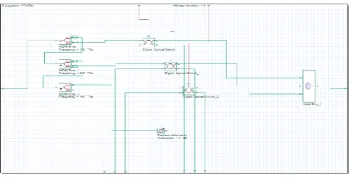
The following figure 5 shows the Opti-System implementation for 3 COADM, with equivalent number of control signals. It has 6 input frequencies consisting of 190 THz, 192 THz, 194 THz, 202 THz, 204 THz and 206 THz while 6 other frequencies can be added as optional depending on the losses. The frequencies that can be added are 196 THz, 198 THz, 200 THz, 208 THz, 210 THz and 212 THz. These frequencies are selected because they lie in the operating wavelength window of 1580 nm for the optical fibre. The below figure 5 and 6 shows the internal design and whole topology for 3 COADM.

[image:3.595.307.550.275.404.2]

Fig. 5 Internal design of 3 switching COADM For the implementation of larger topology and for the analysis of results as the number of nodes increases, 2 COADM was considered and the number nodes was increased from six nodes to ten nodes that were added for extension. The Fig. 6 shows the external connections present in the 6 node COADM network. Here the first two nodes taken as source nodes.

Fig. 6. 6 nodes network of 3 COADM III. RESULTS

The integration of the two phases means that the Machine Learning is implemented to each and every node and the output links from the node will be predicted. Here in Optical topology the links are in the form of Frequency carriers thus, it will give rise to Frequency re-use concept. It can be observed that with integration of machine learning, the algorithm by itself will select the frequency as per the re-use concept. As use of the same frequency in different nodes will lead to congestion which will be predicted by the algorithm.

Table 2 shows the noise figure in 2 COADM network at various nodes without and with Random Forest (RF) algorithms respectively. It can be observed that there is reduction in Noise Figure after the application of the Random Forest algorithms in 2 COADM network compared to 2 COADM network without Random Forest Algorithm in the network as shown in the Table 3.

Table 2. Noise Figure in 2 COADM without RF (Itr. 0) with RF (Itr. 1, 2)

Nodes Frequency Iteration 0 Iteration 1 Iteration 2

Node 3 194 100 42.008 35.97

196 176.54 41.99 1.91

Node 4 202 169.19 41.99 35.97

204 170.512 42.00 35.97

Node 5 190 100 73.45 71.41

192 88.17 0.035 95.62

[image:3.595.63.276.542.644.2]

(4)

[image:4.595.307.546.50.95.2]

198 95.61 2.00 1.97

Table 3. Performance (difference in Noise Fig.) in 2 COADM

Nodes Frequency Loss 1 Loss 2

Node 3 194 57.99 6.02

196 134.54 40.08

Node 4 202 127.19 6.08

204 128.51 -6.02

Node 5 190 26.54 2.03

192 88.13 -95.58

Node 6 194 82.08 -42.78

198 93.61 0.02

The above noise figures have been graphically represented for the selected frequencies in the following figure 7.

Fig. 7 Noise Figures for the selected frequencies. Similarly, Table 4 and Table 5 shows the noise figure in 3 COADM network at various nodes without and with Random Forest algorithms respectively.

Node 3 196 63.91 62.79 61.79

198 100 73.13 77.14

200 80.89 1.96 1.90

Node 4 208 71.03 68.55 54.37

210 163.76 1.95 1.89

212 163.21 1.95 1.90

Node 5 190 46.22 5.32 23.57

192 93.87 83.16 80.17

194 82.64 77.62 77.60

Node 6 194 48.5 36.04 34.79

202 89.16 0.738 2.16

204 44.16 5.99 1.92

Node 3 196 1.12 0.99

198 26.86 -4.01

200 78.92 0.06

Node 4 208 2.48 14.17

210 161.81 0.05

212 161.25 0.05

Node 5 190 40.89 -18.25

192 10.70 2.99

194 5.01 0.023

Node 6 194 12.53 1.25

202 88.42 -1.42

204 38.17 -0.02

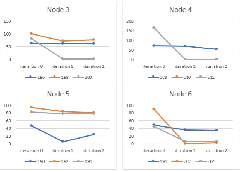
[image:4.595.306.548.150.322.2]

The above noise figures have been graphically represented for the selected frequencies in the following figure 8.

[image:4.595.49.291.229.404.2]

Fig. 8 Noise Figures for the selected frequencies. Similarly, Table 6 and Table 7 show the noise figure in 4 COADM network at various nodes without and with Random Forest algorithms respectively.

Node 3 196 63.91 62.79 61. 79

198 100 73.13 77.14

200 80.89 1.96 1.90

Node 4 208 71.03 68.55 54.37

210 163.76 1.95 1.89

212 163.21 1.95 1.90

Node 5 190 46.22 5.32 23.57

192 93.87 83.16 80.17

194 82.64 77.62 77.60

Node 6 194 48.58 36.04 34.79

202 89.16 0.73 2.16

[image:4.595.310.547.601.831.2]

204 44.16 5.99 6.01

Node 3 196 1.12 0.99

198 26.86 -4.01

200 78.92 0.06

Node 4 208 2.48 14.17

210 161.81 0.05

212 161.25 0.05

Node 5 190 40.89 -18.25

192 10.70 2.99

194 5.01 0.02

Node 6 194 12.53 1.25

202 88.42 -1.42

(5)

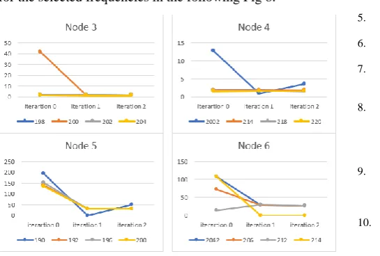
[image:5.595.48.321.70.254.2]

The above noise figures have been graphically represented for the selected frequencies in the following Fig 8.

Fig.8. Noise Figures for the selected frequencies. IV. CONCLUSIONS

This paper proposes the selection of ML algorithm to predict the traffic for a defined set of database and switches the traffic using COADM. Here supervised learning has been used for the defined dataset. Selection of algorithms depends completely on the type of training data and its application. Here the machine learning algorithms are used to predict the future traffic so that by the time the actual data traffic comes, the network will know the links to forward it. Three of the ML algorithms were used for the experiment, testing which: SVM is the best algorithm with 100% accuracy but takes large amount of time to learn the data and reduces the over-all performance of the network. kNN, though is simple cannot classify if any part of the data is missing. Thus, Random Forest can be concluded to be the most optimistic algorithm for the given dataset and given scenario. The algorithms were applied twice for the dataset, and the results were tabulated for 3 iterations (1 without ML and 2 with ML) which gives the performance observed based on the reduction in Noise Figure. This Noise Figure is improved by 42% and 35% in iteration 2 and 3 compared to iteration1 and around 15% from iteration 3 compared to iteration 2 taken from Table 2. When ML algorithm is applied to the Node the Noise Figure will reduce it also depends on the traffic at that link at a given time. It has been observed that as number of frequencies increases, efficiency of ML decreases. This when applied to every node of the network will improve the over-all performance of the network.

ACKNOWLEDGMENT

The authors gratefully acknowledge the help extended by Mr. K. Viswavardhan Reddy (Assistant Professor, RVCE) during the completion of this project.

REFERENCES

1. Francesco Musumeci, Cristina Rottondi, et. al “An Overview on Application of Machine LearningTechniques in Optical Networks”, in IEEE Communications Surveys & Tutorial, Vol 21, Issue:2, PP No. 1383-1408, 08 November 2018.

2. A. L. Buczak and E. Guven, “A survey of data mining and machine learning methods for cyber security intrusion detection,” IEEE Communications Surveys & Tutorials, vol. 18, no. 2, pp. 1153–1176, Oct. 2015.

3. T. T. Nguyen and G. Armitage, “A survey of techniques for internet traffic classification using machine learning,” IEEE Communications Surveys & Tutorials, vol. 10, no. 4, pp. 56–76, 4th Q 2008.

4. M. Bkassiny, Y. Li, and S. K. Jayaweera, “A survey on machine learning techniques in cognitive radios,” IEEE Communications Surveys & Tutorials, vol. 15, no. 3, pp. 1136–1159, Oct. 2012. 5. B. Mukherjee,Optical WDM networks. Springer Science &

BusinessMedia, 2006.

6. S. Ramamurthy and B. Mukherjee, “Survivable WDM mesh networks.

7. Part I-Protection,” in Eighteenth Annual Joint Conference of the IEEE Computer and Communications Societies (INFOCOM) 1999, vol. 2, Mar. 1999, pp. 744–751.

8. Weiyang Mo, Craig L. Gutterman, Yao Li, Shengxiang Zhu, Gil Zussman, and Daniel C. Kilper, "Deep-Neural-Network-Based Wavelength Selection and Switching in ROADM Systems" Journal of Optical Communications and Networking Vol. 10, Issue 10, pp. D1- D11, 2018.

9. B. C. Chatterjee, N. Sarma, and E. Oki, “Routing and spectrum allocation in elastic optical networks: A tutorial,” IEEE Communications Surveys & Tutorials, vol. 17, no. 3, pp. 1776–1800, 2015.

10. Y. Huang, P. B. Cho, P. Samadi, and K. Bergman, “Dynamic power pre-adjustments with machine learning that mitigate EDFA excursions during defragmentation,” in Optical Fiber Communications Conf. and Exhibition (OFC), Mar. 2017, pp. 1–3. 11. D. Rafique, T. Szyrkowiec, H. Grießer, A. Autenrieth, and J.-P.

Elbers, “Cognitive assurance architecture for optical network fault management,” J. Lightwave Technol., vol. 36, no. 7, pp. 1443–1450, Apr. 2018.

12. A. P. Vela, B. Shariati, M. Ruiz, F. Cugini, A. Castro, H. Lu, R. Proietti, J. Comellas, P. Castoldi, S. J. B. Yoo, and L. Velasco, “Soft failure localization during commissioning testing and lightpath operation,” J. Opt. Commun. Netw., vol. 10, no. 1, pp. A27–A36, Jan. 2018.

13. Y. Huang, P. B. Cho, P. Samadi, and K. Bergman, “Dynamic power pre-adjustments with machine learning that mitigate EDFA excursions during defragmentation,” in Optical Fiber Communications Conf. and Exhibition (OFC), Mar. 2017, pp. 1–3. 14. https://medium .com / @ williamkoehrsen/random-forest-simple-

explanation - 377895a60d2d

15. https://medium.com/@equipintelligence/k-nearest-neighbor- classifier - knn-machine-learning-algorithms-ed62feb86582

16. https://www.saedsayad.com/support_vector_machine.htm

AUTHORS PROFILE

Ms. Divya Khanure has completed B.E. degree from SDM College of Engineering and Technology, Dharwad. And has received the degree of M.Tech from RV College of engineering, Bengaluru. The Master degree being aspired in the field of Digital Communications in the dept of Telecommunication.