Double-resonance magnetometry in arbitrarily oriented fields

(1)

Double-Resonance

Magnetometry in Arbitrarily

Oriented Fields

Stuart Ingleby

(2)

Overview

• Quantum Technology Hub

–

 

Practical focus: apply QT to sensors

• Design choices

–

 

Unshielded sensor

• B

₀

orientation

–

 

Signal amplitude and phase effects

• Exploitation

–

 

Demonstrator system

(3)

• Led Birmingham University

–

 

Includes Strathclyde, Nottingham,

Sussex, Southampton, NPL &

industry

–

 

Started Jan 2015

• Unshielded portable sensor

–

 

Geophysical measurement

–

 

Low size, power requirement

–

 

Sub-pT sensitivity

(4)

Unshielded Double

Resonance Sensor

• Dynamic range - yes

– 

No requirement for µT compensation

• Noise rejection - yes

– 

Homodyne detection

– 

Polarimetry

– 

Gradiometry

• Arbitrary B

₀

orientation - ?

– 

Dead-zones

– 

Heading errors

• Portability - yes

– 

Single frequency pump-probe

– 

Firmware signal processing

(5)

Unshielded Double

Resonance Sensor

• Dynamic range - yes

– 

No requirement for µT compensation

• Noise rejection - yes

– 

Homodyne detection

– 

Polarimetry

– 

Gradiometry

• Arbitrary B

₀

orientation - ?

– 

Dead-zones

– 

Heading errors

• Portability - yes

– 

Single frequency pump-probe

– 

Firmware signal processing

(6)

[image:6.720.47.715.29.421.2]

INGLEBY, O’DWYER, GRIFFIN, ARNOLD, AND RIIS PHYSICAL REVIEW A 96, 013429 (2017)

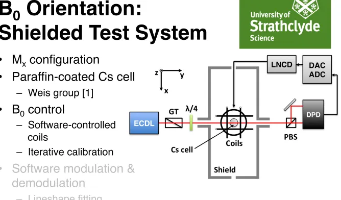
FIG. 1. Schematic of the apparatus used in this work, show-ing external cavity diode laser (ECDL), Glan-Thompson linear polarizer (GT), quarter-wave plate (λ/4), magnetometer cell,

five-layer mu-metal shield, three-axis Helmholtz coils, polarizing beam splitter (PBS), differential photodetector (DPD), low-noise coil driver (LNCD), and data acquisition system (DAC/ADC). The data acquisition system is controlled using a PC (not shown).

writing

ρ =

2F

!

k₌0 k

!

q₌₋k

mk,qT_q(k), (1)

where T_q(k) are irreducible basis tensors in the chosen

quantization basis. We consider a three-stage process to derive the observed polarimeter signal; the creation of atomic magnetization through optical pumping, the evolution of that magnetization in the magnetic field, and the observable effects on transmitted light. This three-stage model is only valid in the case of weak optical pumping (where the optical pumping rate is much smaller than the magnetic spin relaxation rate), in which the evolution of the magnetization (stage two) can be considered due to the action of magnetic fields only.

Figure 2 shows the coordinate basis used to describe the laboratory frame. If the quantization axis is parallel to the k

vector of the pump light, then nonabsorbing atomic dark states are described by sums of atomic multipoles in which onlymk,0

moments are nonzero, wherek may be any positive integer for

circularly polarized light and k any even positive integer for

linearly polarized light [19]. Optical pumping dynamically couples multipole moments of any k,q to moments for which q = 0 in this basis. In a static magnetic field the resulting

equilibrium moments meq_k,q depend on the rate of optical

pumping and the orientation of the static field B0 [19].

Our magnetometer signal is the oscillating magnetization response to BRF(ωRF), so we define a rotating wave frame x′ −y′ −z′(RW) such thatB0lies alongz′, and the component

ofBRF perpendicular toB0 at t = 0, B_RF⊥ , is in the negative x′

direction. In the presence of weak optical pumping, the atomic polarization relaxes to states which are symmetric around the quantization axis B0, in which only m′_k,eq₀ are nonzero.

The evolution of mk,q in the presence of a magnetic field

was derived from the Liouville equation in [18] and is given by

d

dtmk,q =

!

q′

O(_qqk)′mk,q′ − $ (k) qq′

"

mk,q′ −m eq k,q′

#

, (2)

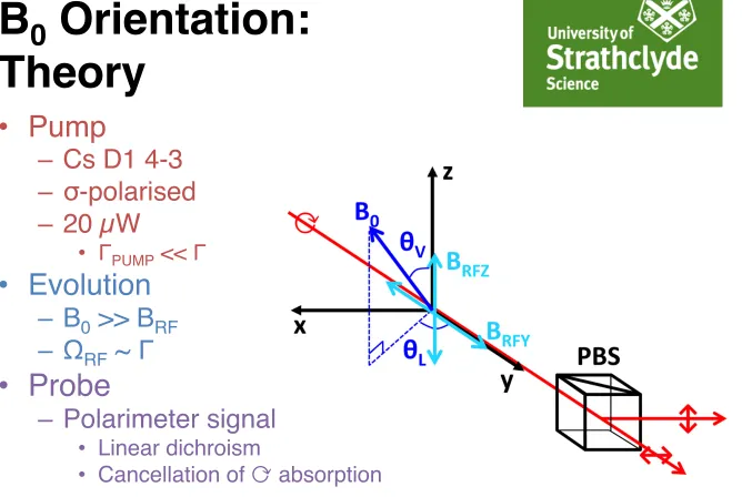
FIG. 2. Schematic showing the geometry of the magnetometer system in the laboratory frame. The orientation of the static fieldB0

is defined by the angles to the light propagation and vertical axes,

θL and θV, respectively. Inset, alternative polar basis angles α and β

are defined. The orientations of the oscillating fieldsBRF Z andBRF Y,

and the polarization analyser (PBS), are also shown.

where O(_qqk)′ is a (2k +1) ×(2k +1) matrix describing the

action ofB0andBRF onmk,q and$_qq(k)′ is a (2k + 1)× (2k + 1)

matrix describing the relaxation of mk,q to meq_k,q. By solving

for equilibrium multipole moments in the RW framem′_k,q and

transforming to the laboratory frame, we obtain expressions for the oscillating components of mk,q(t). Transformations of mk,q(t) under rotation are obtained using Wigner D matrices

(see [20] for details).

A balanced polarimeter is used for these measurements, ensuring that the observed signal is sensitive to relative changes in the transmission of orthogonal linearly polarized light through the cell. Signal contributions due to oscillating transmission of circularly polarized light will be observed in-phase on both polarimeter channels and will not contribute to the measured differential signal. The measured signal is thus modeled by the difference in absorption of the orthogonal linear polarization states of the light received at the polarization analyser (see Fig. 2). The absorption coefficient κ for linearly

polarized light in a medium described by multipole moments

mk,q(t) is proportional to

κ ∝ √A0

3m0,0 −

$

2

3A2m2,0, (3) where A0 and A2 are analyzing powers [18]. The analyzing

powersA0,A2, and monopole momentm0,0are invariant under

rotations of basis, and cancel in subtraction, so we can write a function f(t) which is proportional to the polarimeter signal,

f(t) = m2,0(t) −m′′₂_,₀(t)

= 3₂m2,0(t) −

%

3

8[m2,2(t) + m2,₋2(t)], (4)

where mk,q(t) denotes multipole moments in the laboratory

frame and m′′_k,q(t) multipole moments in a frame rotated such

that the quantization axis is coincident with the orthogonal

013429-2

B

₀

Orientation:

 

Shielded Test System

• M

_x

configuration

• Paraffin-coated Cs cell

– 

Weis group [1]

• B

₀

control

– 

Software-controlled

coils

– 

Iterative calibration

• Software modulation &

demodulation

–

 

Lineshape fitting

20/08/17 Stuart Ingleby - Strathclyde University 6

(7)

[image:7.720.47.713.31.478.2]

INGLEBY, O’DWYER, GRIFFIN, ARNOLD, AND RIIS PHYSICAL REVIEW A 96, 013429 (2017)

writing

ρ =

2F !

k₌0 k !

q₌₋k

mk,qT_q(k), (1)

moments are nonzero, wherek may be any positive integer for

linearly polarized light [19]. Optical pumping dynamically couples multipole moments of any k,q to moments for which q = 0 in this basis. In a static magnetic field the resulting

Our magnetometer signal is the oscillating magnetization response to BRF(ωRF), so we define a rotating wave frame

x′ −y′ −z′(RW) such thatB0lies alongz′, and the component

ofBRF perpendicular toB0 at t = 0, B_RF⊥ , is in the negative x′

direction. In the presence of weak optical pumping, the atomic polarization relaxes to states which are symmetric around the quantization axis B0, in which only m′_k,eq₀ are nonzero.

d

dtmk,q =

!

q′

O(_qqk)′mk,q′ − $

(k) qq′

"

#

, (2)

action ofB0andBRF onmk,q and$_qq(k)′ is a (2k + 1)× (2k + 1)

for equilibrium multipole moments in the RW framem′_k,q and

transforming to the laboratory frame, we obtain expressions for the oscillating components of mk,q(t). Transformations of

mk,q(t) under rotation are obtained using Wigner D matrices

κ ∝ √A0

3m0,0 −

$

2

3A2m2,0, (3) where A0 and A2 are analyzing powers [18]. The analyzing

powersA0,A2, and monopole momentm0,0are invariant under

f(t) = m2,0(t) −m′′₂_,₀(t)

= 3₂m2,0(t) − %

3

8[m2,2(t) + m2,₋2(t)], (4)

013429-2

B

₀

Orientation:

 

Shielded Test System

• M

_x

configuration

• Paraffin-coated Cs cell

–

 

Weis group []

• B

₀

control

–

 

Software-controlled

coils

–

 

Iterative calibration

• Software modulation &

demodulation

– 

Lineshape fitting

Figure 4: Variation of relaxation rate, sensitivity (unshielded NEP) and signal amplitude with varying modulation depth.

Although signal amplitude is, to first order, proportional to modulation depth, resonance width increases when BRF.gF ~ Γ. Measurement of sensitivity with varying modulation depth identified a range of suitable magnitudes for BRF.

Figure 5: Shielded and unshielded magnetic resonances observed with optimised field gradient, orientation and modulation depth.

Figure 5 shows the amplitudes of demodulated in-phase (X) and quadrature components (Y) of the polarisation rotation response to field modulation depth of 1 nT (7 nT unshielded). The estimated magnetometric sensitivity is 173 fT.Hz-1/2 (19.6 pT.Hz-1/2 unshielded).

By creating PID-controlled feedback from the in-phase signal to the

(8)

B

₀

Orientation:

 

Shielded Test System

• B

₀

control

• Low-noise current

drivers

– 

Shield degauss

– 

Single-axis calibration

[2]

– 

3D calibration

[C. O’Dwyer poster]

• 200 nT B

₀

–  δ

|B| = 0.24 nT

–  δθ

= 0.23 mrad

B₀ (µT)

(9)

INGLEBY, O’DWYER, GRIFFIN, ARNOLD, AND RIIS PHYSICAL REVIEW A96, 013429 (2017)

writing

ρ =

2F !

k₌0 k !

q₌₋k

mk,qT_q(k), (1)

vector of the pump light, then nonabsorbing atomic dark states are described by sums of atomic multipoles in which onlymk,0 moments are nonzero, wherek may be any positive integer for

linearly polarized light [19]. Optical pumping dynamically couples multipole moments of anyk,q to moments for which q ₌ 0 in this basis. In a static magnetic field the resulting

pumping and the orientation of the static fieldB0 [19].

x′ ₋y′ ₋z′(RW) such thatB0lies alongz′, and the component

of BRF perpendicular toB0 att = 0, B_RF⊥ , is in the negative x′ direction. In the presence of weak optical pumping, the atomic polarization relaxes to states which are symmetric around the quantization axis B0, in which only m′_k,eq₀ are nonzero.

The evolution of mk,q in the presence of a magnetic field was derived from the Liouville equation in [18] and is given by

d

dtmk,q =

!

q′

O(_qqk)′mk,q′ −$_qq(k)′

"

#

[image:9.720.45.713.28.476.2]

, (2)

θL andθV, respectively. Inset, alternative polar basis angles α and β

action ofB0andBRF onmk,q and$

(k)

qq′ is a (2k +1) ×(2k +1) matrix describing the relaxation of mk,q to m

eq

k,q. By solving for equilibrium multipole moments in the RW frame m′_k,q and

mk,q(t) under rotation are obtained using Wigner D matrices (see [20] for details).

A balanced polarimeter is used for these measurements, ensuring that the observed signal is sensitive to relative changes in the transmission of orthogonal linearly polarized light through the cell. Signal contributions due to oscillating transmission of circularly polarized light will be observed in-phase on both polarimeter channels and will not contribute to the measured differential signal. The measured signal is thus modeled by the difference in absorption of the orthogonal linear polarization states of the light received at the polarization analyser (see Fig.2). The absorption coefficient κ for linearly polarized light in a medium described by multipole moments

κ ∝ √A0

3m0,0 − $

2

3A2m2,0, (3)

where A0 and A2 are analyzing powers [18]. The analyzing

powersA0,A2, and monopole momentm0,0are invariant under rotations of basis, and cancel in subtraction, so we can write a function f(t) which is proportional to the polarimeter signal,

f(t) = m2,0(t)−m′′₂_,₀(t)

= 32m2,0(t)− %

3

8[m2,2(t) +m2,₋2(t)], (4) where mk,q(t) denotes multipole moments in the laboratory frame and m′′_k,q(t) multipole moments in a frame rotated such

013429-2

B

₀

Orientation:

 

Theory

• Pump

–

 

Cs D1 4-3

–

  σ

-polarised

–

 

20 µW

•  Γ

_PUMP

<<

Γ

• Evolution

– 

B

₀

>> B

_RF

–  Ω

_RF

~

Γ

• Probe

–

 

Polarimeter signal

• Linear dichroism

• Cancellation of ⟳ absorption

(10)

writing

ρ =

2F !

k₌0 k !

q₌₋k

mk,qT_q(k), (1)

vector of the pump light, then nonabsorbing atomic dark states are described by sums of atomic multipoles in which onlymk,0 moments are nonzero, wherek may be any positive integer for

linearly polarized light [19]. Optical pumping dynamically couples multipole moments of anyk,q to moments for which q ₌ 0 in this basis. In a static magnetic field the resulting

pumping and the orientation of the static fieldB0 [19].

x′ ₋y′ ₋z′(RW) such thatB0lies alongz′, and the component

of BRF perpendicular toB0 att = 0, B_RF⊥ , is in the negative x′ direction. In the presence of weak optical pumping, the atomic polarization relaxes to states which are symmetric around the quantization axis B0, in which only m′_k,eq₀ are nonzero.

The evolution of mk,q in the presence of a magnetic field was derived from the Liouville equation in [18] and is given by

d

dtmk,q =

!

q′

O(_qqk)′mk,q′ −$_qq(k)′

"

#

, (2)

θL andθV, respectively. Inset, alternative polar basis angles α and β

(k)

qq′ is a (2k +1) ×(2k +1) matrix describing the relaxation of mk,q to m

eq

k,q. By solving for equilibrium multipole moments in the RW frame m′_k,q and

mk,q(t) under rotation are obtained using Wigner D matrices (see [20] for details).

A balanced polarimeter is used for these measurements, ensuring that the observed signal is sensitive to relative changes in the transmission of orthogonal linearly polarized light through the cell. Signal contributions due to oscillating transmission of circularly polarized light will be observed in-phase on both polarimeter channels and will not contribute to the measured differential signal. The measured signal is thus modeled by the difference in absorption of the orthogonal linear polarization states of the light received at the polarization analyser (see Fig.2). The absorption coefficient κ for linearly polarized light in a medium described by multipole moments

κ ∝ √A0

3m0,0 − $

2

3A2m2,0, (3)

where A0 and A2 are analyzing powers [18]. The analyzing

powersA0,A2, and monopole momentm0,0are invariant under rotations of basis, and cancel in subtraction, so we can write a function f(t) which is proportional to the polarimeter signal,

f(t) = m2,0(t)−m′′₂_,₀(t)

= 32m2,0(t)− %

3

8[m2,2(t) +m2,₋2(t)], (4) where mk,q(t) denotes multipole moments in the laboratory frame and m′′_k,q(t) multipole moments in a frame rotated such

013429-2

B

₀

Orientation:

 

Theory

Multipole moment model

[3][4]

• Pump

– 

Creation of

k = 1,2

…

– 

Equilibrium

q = 0

• B

₀

frame

• Evolution

–

 

RW frame

• B

₀

// z

• B

_RF

(t=0) // -x

–

 

Obtain

m

_kq

(t)

• Probe

–

 

Difference in

↕

︎

and

↔

︎

writing

ρ =

2F

!

k₌0 k

!

q₌₋k

mk,qT_q(k), (1)

where T_q(k) are irreducible basis tensors in the chosen quantization basis. We consider a three-stage process to derive the observed polarimeter signal; the creation of atomic magnetization through optical pumping, the evolution of that magnetization in the magnetic field, and the observable effects on transmitted light. This three-stage model is only valid in the case of weak optical pumping (where the optical pumping rate is much smaller than the magnetic spin relaxation rate), in which the evolution of the magnetization (stage two) can be considered due to the action of magnetic fields only.

Figure 2 shows the coordinate basis used to describe the laboratory frame. If the quantization axis is parallel to the k vector of the pump light, then nonabsorbing atomic dark states are described by sums of atomic multipoles in which onlymk,0

moments are nonzero, wherek may be any positive integer for circularly polarized light and k any even positive integer for linearly polarized light [19]. Optical pumping dynamically couples multipole moments of any k,q to moments for which q ₌ 0 in this basis. In a static magnetic field the resulting equilibrium moments meq_k,q depend on the rate of optical pumping and the orientation of the static field B0 [19].

x′ −y′ −z′(RW) such thatB₀lies alongz′, and the component ofBRF perpendicular toB0 att = 0,B_RF⊥ , is in the negativex′

direction. In the presence of weak optical pumping, the atomic polarization relaxes to states which are symmetric around the quantization axis B₀, in which only m′_k,eq₀ are nonzero.

d

dtmk,q =

!

q′

O(_qqk)′mk,q′ −$( k) qq′

"

#

, (2)

FIG. 2. Schematic showing the geometry of the magnetometer system in the laboratory frame. The orientation of the static fieldB0 is defined by the angles to the light propagation and vertical axes, θL andθV, respectively. Inset, alternative polar basis angles α andβ are defined. The orientations of the oscillating fieldsBRF Z andBRF Y, and the polarization analyser (PBS), are also shown.

where O(_qqk)′ is a (2k +1)×(2k+1) matrix describing the

action ofB0andBRF onmk,q and$( k)

qq′ is a (2k+1)×(2k+1)

matrix describing the relaxation of mk,q to m eq

k,q. By solving

for equilibrium multipole moments in the RW framem′_k,q and transforming to the laboratory frame, we obtain expressions for the oscillating components of mk,q(t). Transformations of

mk,q(t) under rotation are obtained using Wigner D matrices

A balanced polarimeter is used for these measurements, ensuring that the observed signal is sensitive to relative changes in the transmission of orthogonal linearly polarized light through the cell. Signal contributions due to oscillating transmission of circularly polarized light will be observed in-phase on both polarimeter channels and will not contribute to the measured differential signal. The measured signal is thus modeled by the difference in absorption of the orthogonal linear polarization states of the light received at the polarization analyser (see Fig.2). The absorption coefficient κ for linearly polarized light in a medium described by multipole moments mk,q(t) is proportional to

κ ∝ √A0

3m0,0 −

$

2

3A2m2,0, (3) where A₀ and A₂ are analyzing powers [18]. The analyzing powersA0,A2, and monopole momentm0,0are invariant under

rotations of basis, and cancel in subtraction, so we can write a functionf(t) which is proportional to the polarimeter signal,

f(t) ₌ m₂_,₀(t)₋m′′₂_,₀(t) = 3₂m2,0(t)−

%

3

8[m2,2(t)+m2,₋2(t)], (4)

frame andm′′_k,q(t) multipole moments in a frame rotated such that the quantization axis is coincident with the orthogonal

013429-2

FIG. 1. Schematic of the apparatus used in this work, show-ing external cavity diode laser (ECDL), Glan-Thompson linear polarizer (GT), quarter-wave plate (λ/4), magnetometer cell, five-layer mu-metal shield, three-axis Helmholtz coils, polarizing beam splitter (PBS), differential photodetector (DPD), low-noise coil driver (LNCD), and data acquisition system (DAC/ADC). The data acquisition system is controlled using a PC (not shown).

writing

ρ ₌

2F

!

k₌0 k

!

q₌₋k

mk,qT_q(k), (1)

moments are nonzero, wherekmay be any positive integer for

linearly polarized light [19]. Optical pumping dynamically couples multipole moments of anyk,q to moments for which q = 0 in this basis. In a static magnetic field the resulting

Our magnetometer signal is the oscillating magnetization response to BRF(ωRF), so we define a rotating wave frame x′ ₋y′ ₋z′(RW) such thatB0lies alongz′, and the component ofBRF perpendicular to B0 att = 0,B_RF⊥ , is in the negativex′

direction. In the presence of weak optical pumping, the atomic polarization relaxes to states which are symmetric around the quantization axisB0, in which only m′_k,eq₀ are nonzero.

d

dt mk,q =

!

q′

O(_qqk)′mk,q′ −$

(k) qq′

"

#

, (2)

FIG. 2. Schematic showing the geometry of the magnetometer system in the laboratory frame. The orientation of the static field B0

θL and θV, respectively. Inset, alternative polar basis angles α andβ

where O(_qqk)′ is a (2k+1)×(2k+1) matrix describing the

(k)

qq′ is a (2k+1)×(2k+1)

for equilibrium multipole moments in the RW frame m′_k,q and

A balanced polarimeter is used for these measurements, ensuring that the observed signal is sensitive to relative changes in the transmission of orthogonal linearly polarized light through the cell. Signal contributions due to oscillating transmission of circularly polarized light will be observed in-phase on both polarimeter channels and will not contribute to the measured differential signal. The measured signal is thus modeled by the difference in absorption of the orthogonal linear polarization states of the light received at the polarization analyser (see Fig. 2). The absorption coefficientκ for linearly

κ _∝ _√A0

3m0,0 −

$

2

3A2m2,0, (3) where A0 and A2 are analyzing powers [18]. The analyzing powersA0,A2, and monopole momentm0,0are invariant under

f(t) ₌ m2,0(t)−m′′₂_,₀(t)

= 32m2,0(t)−

%

3

8[m2,2(t)+m2,₋2(t)], (4)

013429-2

writing

ρ =

2F

!

k₌0 k

!

q₌₋k

mk,qT_q(k), (1)

vector of the pump light, then nonabsorbing atomic dark states are described by sums of atomic multipoles in which onlym_k,₀

moments are nonzero, wherekmay be any positive integer for

linearly polarized light [19]. Optical pumping dynamically couples multipole moments of anyk,q to moments for which q = 0 in this basis. In a static magnetic field the resulting

pumping and the orientation of the static fieldB₀ [19].

Our magnetometer signal is the oscillating magnetization response to BRF(ωRF), so we define a rotating wave frame x′ ₋y′ ₋z′(RW) such thatB₀lies alongz′, and the component

ofB_RF perpendicular toB₀ at t ₌0,B_RF⊥ , is in the negativex′

direction. In the presence of weak optical pumping, the atomic polarization relaxes to states which are symmetric around the quantization axis B0, in which onlym′_k,eq₀ are nonzero.

d

dtmk,q =

!

q′

O(_qqk)′mk,q′ −$( k) qq′

"

#

, (2)

where O(_qqk)′ is a (2k +1)×(2k +1) matrix describing the

action ofB0andBRF onmk,q and$( k)

qq′ is a (2k +1)×(2k +1)

matrix describing the relaxation of m_k,q to meq_k,q. By solving

for equilibrium multipole moments in the RW frame m′_k,q and

κ _∝ _√A0

3m0,0 − $

2

3A2m2,0, (3) where A₀ and A₂ are analyzing powers [18]. The analyzing

powersA₀,A₂, and monopole momentm₀,0are invariant under

rotations of basis, and cancel in subtraction, so we can write a functionf(t) which is proportional to the polarimeter signal,

f(t) = m2,0(t)−m′′₂_,₀(t)

= 32m2,0(t)−

% 3

8[m2,2(t)+m2,₋2(t)], (4)

where m_k,q(t) denotes multipole moments in the laboratory

013429-2

(11)

B

₀

Orientation:

 

Amplitude

•  

4 π

angular scan

–

 

1646 resonance fits

–

 

3 ½

hours

• R

–

 

Extract X and Y

from f(t)

• Dead-zones

INGLEBY, O’DWYER, GRIFFIN, ARNOLD, AND RIIS

PHYSICAL REVIEW A

96 , 013429 (2017)

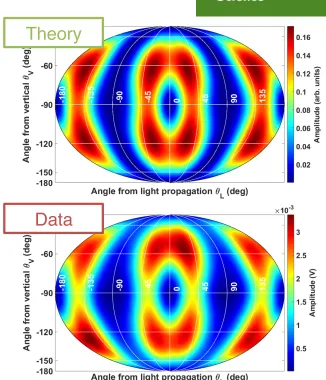
FIG. 5. Calculated (top) and observed (bottom) distribution of

on-resonance first-harmonic polarimeter signal phase over 4

π

solid

angle in response to a field modulation

B

_RF

applied parallel to the

light propagation (

y

) axis.

where cos

β

=

sin

θ

_V

cos

θ

_L

and tan

α

=

tan

θ

_V

sin

θ

_L

define

an alternative polar basis in the laboratory frame.

In practical magnetometry measurements we are concerned

with the amplitude

R

and phase

φ

of the magnetometer signal

response. Defining

R

2 ≡

X

2 +

Y

2 ,

(11)

tan

φ

≡

X/Y,

(12)

we obtain on-resonance signal amplitudes

R

_{RF y}

2 =

A

2 sin

2

2 β

(cos

2 β

cos

2

2 α

+

sin

2

2 α

)

,

(13)

R

_{RF z}

2 =

A

2 sin

4 θ

_V

[4 cos

2 θ

_V

(1

+

cos

2 θ

_L

)

2 +

sin

2

2 θ

_L

]

,

(14)

and phases

tan

φ

_{RF y}

=

−

2 sin 2

α

sin

β

cos 2

α

sin 2

β

=

_(sin

₂

2 sin

θ

L

tan

θ

V

θ

_L

tan

2 θ

_V

−

1) cos

θ

_L

sin

θ

_V

,

(15)

tan

φ

_{RF z}

=

−

sin 2

θ

L

sin

θ

V

(1

₊

cos

2 _θ

L

) sin 2

θ

V

,

(16)

where

A

=

3 m

′eq

2,0

S

4(4

S

2

+

1)

.

Using the

B

₀

control, signal demodulation, and resonance

line-shape fitting described in [

15 ], angular scans of the

FIG. 6. Calculated (top) and observed (bottom) distribution of

on-resonance first-harmonic polarimeter signal phase over 4

π

solid

angle in response to a field modulation

B

_RF

applied parallel to the

vertical (

z

) axis.

measured on-resonance signal amplitude

R

and phase

φ

were

made. Each angular scan comprised 1646 varying orientations

of

B

₀

=

200 nT spread with equal angular density over the full

4 π

solid angle. Figures

3 –

6 show these data plotted alongside

distributions calculated using Eqs. (

13 )–(

16 ).

IV. CONCLUSIONS

Equations (

13 ) and (

14 ) model the observed dead-zones

(orientations of

B

₀

for which

R

→

0) and symmetries in

the distribution of observed signal amplitude

R

(Figs.

3 and

4 ). We note that our experimental measurements of signal

amplitude differ slightly in shape to the predicted distributions,

a feature which could be reduced by inclusion of

higher-order multipole moments in the model signal calculation. In

the case where the polarimeter is not perfectly balanced, the

signal contribution due to the evolution of first-order multipole

moments

m

₁

_,q

, which modulate the transmission of circularly

polarized light, will not be fully canceled by the differential

photodetector. This may also account for discrepancies

be-tween the observed and calculated distributions of

R

.

Equations (

15 ) and (

16 ) appear to model the observed

polarimeter signal phase well, and the observed data

con-firm the strong correlation of on-resonance phase with

B

₀

orientation (Figs.

5 and

6 ). The clarity and good agreement

of the measured data with calculated signal phase may be

013429-4

[image:11.720.320.646.108.488.2]

ORIENTATIONAL EFFECTS ON THE AMPLITUDE AND . . . PHYSICAL REVIEW A96, 013429 (2017)

FIG. 3. Calculated (top) and observed (bottom) distribution of on-resonance first-harmonic polarimeter signal amplitude over 4π

solid angle in response to a field modulationBRF applied parallel to

the light propagation (y) axis.

linear polarization axis (x axis). Since the orthogonal linear

states separated by the analyzer are not sensitive tom1,q(t) and

m0,0 is constant in time,k =2 for the lowest-order multipole

moments contributing tof(t).

Following [18], and definingx _≡ (γB0 −ωRF)/$andS ≡

γB_RF⊥ /$for convenience, we obtain the following equations of motion for the RW-framek₌2 multipole moments:

i

$m˙ ′

2,q =Mqq′m′₂_,q′ +im′

eq

2,q, (5)

where γ is the gyromagnetic ratio for the Cs 62S1/2 (F =4)

ground state and

Mqq′ =

⎛ ⎜ ⎜ ⎜ ⎜ ⎜ ⎜ ⎜ ⎝

2x ₋i S 0 0 0

S x₋i

$

3

2S 0 0

0 $3₂S ₋i

$

3

2S 0

0 0 $3

2S −x −i S

0 0 0 S ₋2x ₋i

⎞ ⎟ ⎟ ⎟ ⎟ ⎟ ⎟ ⎟ ⎠ . (6)

We have assumed that relaxation in the system is isotropic with rate$, and thatBRF ≪ B0.

Steady-state solutions for m′₂_,q in the RW frame are

obtained by setting ˙m′₂_,q ₌ 0. After transformation to the

laboratory frame we obtain terms ine0iωRFt,e1iωRFt, and_e2iωRFt

the vertical (z) axis.

corresponding to dc, first-harmonic, and second-harmonic resonant magnetization responses to the perturbing fieldBRF.

III. ANISOTROPY IN RESONANT POLARIMETER SIGNAL RESPONSE

To measure the first-harmonic response to BRF(ωRF), the

polarimeter signal is digitized and demodulated in software with a reference phase-locked to BRF(t). Collecting terms

fromf(t) in cos(ωRFt) and sin(ωRFt) we derive expressions

for the in-phase, X, and quadrature, Y, components of the

demodulated signal. The on-resonance (x = 0) amplitudes of X and Y are strongly dependent on the orientation ofB0 and

BRF relative to the light propagation axis. For BRF aligned

along they andzaxes (denoted RFy and RFz, respectively),

XRF y = −

3m′₂eq_,₀S

4S2 ₊1sin 2αsinβ, (7)

YRF y =

3m′₂eq_,₀S

2(4S2 ₊1)cos 2αsin 2β, (8)

XRF z = −

3m′₂eq_,₀S

2(4S2 ₊1) sin 2θLsinθV, (9)

YRF z =

3m′₂eq_,₀S

2(4S2 ₊1)(1+cos

2

θL) sin 2θV, (10)

013429-3

ORIENTATIONAL EFFECTS ON THE AMPLITUDE AND . . . PHYSICAL REVIEW A96, 013429 (2017)

the light propagation (y) axis.

linear polarization axis (x axis). Since the orthogonal linear

states separated by the analyzer are not sensitive tom1,q(t) and

m0,0 is constant in time,k =2 for the lowest-order multipole

moments contributing tof(t).

Following [18], and definingx _≡ (γB0 −ωRF)/$andS ≡

γB_RF⊥ /$for convenience, we obtain the following equations

of motion for the RW-framek₌2 multipole moments: i

$m˙

′

2,q =Mqq′m′₂_,q′ +im′

eq

2,q, (5)

where γ is the gyromagnetic ratio for the Cs 62S1/2 (F =4)

ground state and

Mqq′ = ⎛ ⎜ ⎜ ⎜ ⎜ ⎜ ⎜ ⎜ ⎝

2x ₋i S 0 0 0 S x₋i

$

3

2S 0 0

0 $3₂S −i

$

3

2S 0

0 0 $3

2S −x −i S

0 0 0 S ₋2x ₋i

⎞ ⎟ ⎟ ⎟ ⎟ ⎟ ⎟ ⎟ ⎠ . (6)

We have assumed that relaxation in the system is isotropic with rate$, and thatBRF ≪ B0.

Steady-state solutions for m′₂_,q in the RW frame are

obtained by setting ˙m′₂_,q ₌ 0. After transformation to the

laboratory frame we obtain terms ine0iωRFt,_e1iωRFt, and_e2iωRFt

the vertical (z) axis.

corresponding to dc, first-harmonic, and second-harmonic resonant magnetization responses to the perturbing fieldBRF.

III. ANISOTROPY IN RESONANT POLARIMETER SIGNAL RESPONSE

To measure the first-harmonic response to BRF(ωRF), the

polarimeter signal is digitized and demodulated in software with a reference phase-locked to BRF(t). Collecting terms

fromf(t) in cos(ωRFt) and sin(ωRFt) we derive expressions

for the in-phase, X, and quadrature, Y, components of the

demodulated signal. The on-resonance (x = 0) amplitudes of X and Y are strongly dependent on the orientation ofB0 and

BRF relative to the light propagation axis. For BRF aligned

along they andzaxes (denoted RFy and RFz, respectively),

XRF y = −

3m′₂eq_,₀S

4S2 ₊1sin 2αsinβ, (7) YRF y =

3m′₂eq_,₀S

2(4S2 ₊1)cos 2αsin 2β, (8) XRF z = −

3m′₂eq_,₀S

2(4S2 ₊1) sin 2θLsinθV, (9) YRF z =

3m′₂eq_,₀S

2(4S2 ₊1)(1+cos

2

θL) sin 2θV, (10)

013429-3