City, University of London Institutional Repository
Citation: Wang, W., Härdle, W.K., Cabrera, B.L. & Okhrin, O. (2016). Localising
temperature risk. Journal of the American Statistical Association, doi:10.1080/01621459.2016.1180985
This is the accepted version of the paper.
This version of the publication may differ from the final published
version.
Permanent repository link: http://openaccess.city.ac.uk/15147/
Link to published version: http://dx.doi.org/10.1080/01621459.2016.1180985
Copyright and reuse: City Research Online aims to make research
outputs of City, University of London available to a wider audience.
Copyright and Moral Rights remain with the author(s) and/or copyright
holders. URLs from City Research Online may be freely distributed and
linked to.
City Research Online: http://openaccess.city.ac.uk/ [email protected]
Localising temperature risk
Wolfgang Karl Härdle
∗, Brenda López Cabrera
†, Ostap Okhrin
‡, Weining Wang
§.
April 15, 2016
Abstract
On the temperature derivative market, modelling temperature volatility is an im-portant issue for pricing and hedging. In order to apply the pricing tools of nancial mathematics, one needs to isolate a Gaussian risk factor. A conventional model for temperature dynamics is a stochastic model with seasonality and intertemporal auto-correlation. Empirical work based on seasonality and autocorrelation correction reveals that the obtained residuals are heteroscedastic with a periodic pattern. The object of this research is to estimate this heteroscedastic function so that, after scale nor-malisation, a pure standardised Gaussian variable appears. Earlier works investigated
∗Professor at Humboldt-Universität zu Berlin, Ladislaus von Bortkiewicz chair of statistics and Director of
C.A.S.E. - Center for Applied Statistics and Economics, Humboldt-Universität zu Berlin, Spandauer Straÿe
1, 10178 Berlin, Germany and School of Business, Singapore Management University, 50 Stamford Road,
Singapore 178899. Email:[email protected]
†Assistant professor at the Ladislaus von Bortkiewicz chair of statistics of Humboldt-Universität zu Berlin,
Spandauer Straÿe 1,10178 Berlin, Germany. Email:[email protected]
‡Professor of Statistics and Econometrics at the Faculty of Transportation of Dresden University of
Technology, 01062Dresden, Germany. Email:[email protected]
§Assistant professor at the Ladislaus von Bortkiewicz chair of statistics, Humboldt-Universität zu Berlin,
temperature risk in dierent locations and showed that neither parametric component functions nor a local linear smoother with constant smoothing parameter are exible enough to generally describe the variance process well. Therefore, we consider a local adaptive modelling approach to nd, at each time point, an optimal smoothing param-eter to locally estimate the seasonality and volatility. Our approach provides a more exible and accurate tting procedure for localised temperature risk by achieving nearly normal risk factors. We also employ our model to forecast the temperature in dierent cities and compare it to a model developed in Campbell and Diebold (2005).
Keywords: Weather derivatives, localising temperature residuals, seasonality, local model selection
JEL classication: G19, G29, G22, N23, N53, Q59
1 Introduction
The pricing of contingent claims based on stochastic dynamics, for example, stocks or FX rates, is well known in nancial engineering. An elegant approach to such a pricing task is based on self-nancing replication arguments. An essential element of this approach is the tradeability of the underlying. This however does not apply to weather derivatives, contingent on temperature or rain, since the underlying is not tradeable. In this context, the proposed pricing techniques are based on either equilibrium ideas (Horst and Mueller (2007)) or econometric modelling of the underlying dynamics Campbell and Diebold (2005) and Benth, Benth and Koekebakker (2007) followed by risk neutral pricing.
A time series approach has been taken by Benth et al. (2007), who corrects for seasonality (in mean), then for intertemporal correlation and nally as in Campbell and Diebold (2005), for seasonal variations. After these manipulations, a Gaussian risk factor needs to be isolated in order to apply continuous time pricing techniques, Karatzas and Shreve (2001).
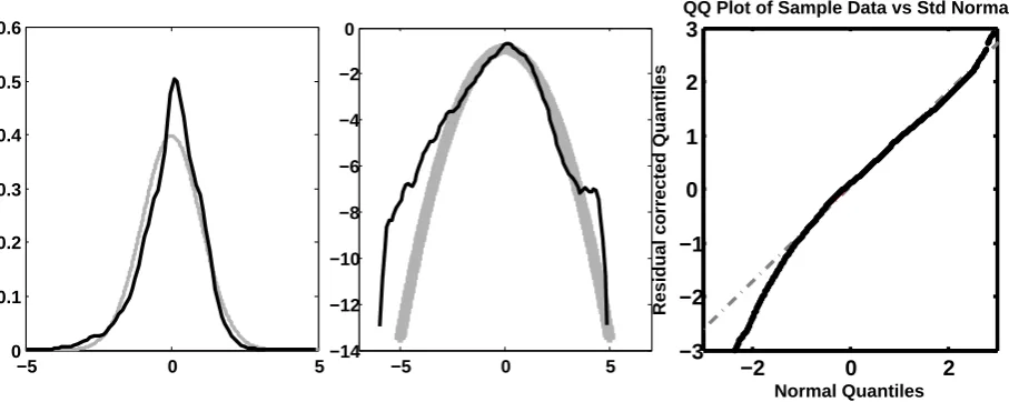
[image:4.595.70.524.358.539.2]Empirical studies following this econometrical route show evidence that the resulting tem-perature risk factor deviates severely from Gaussianity, which in turn challenges the pricing tools, Benth, Härdle and López Cabrera (2011). In particular, for Asian cities, like, for example, Kaohsiung (Taiwan), one observes very distinctive non-normality in the form of clearly visible heavy tails caused by extended volatility in peak seasons. This is visible from Figure 1 where a log density plot reveals a non-normal shoulder structure (kurtosis= 3.22,
skewness=−0.08, JB= 128.74).
−5 0 5
0 0.1 0.2 0.3 0.4 0.5 0.6
−5 0 5
−14 −12 −10 −8 −6 −4 −2 0
−2 0 2
−3 −2 −1 0 1 2 3
Normal Quantiles
Residual corrected Quantiles
QQ Plot of Sample Data vs Std Normal
Figure 1: Kernel density estimates (left panel), log kernel density estimates (middle panel) and QQ-plots (right panel) of normal densities (grey lines) and Kaohsiung standardised residuals (black line)
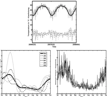
The upper panel of Figure 2 displays the seasonality and deseasonalised residuals over two years in Kaohsiung. The lower panel RHS displays the empirical and smoothed seasonal variance function, while the lower panel LHS shows the smoothed seasonal variance function over years. The Fourier series expansion fails though in the volatility peak seasons. Even incorporating an asymmetry term for the dip of temperature in winter does not improve the closeness to normality. One may of course pursue ne tuning the Fourier method with more and more periodic terms but this will increase the number of parameters; we therefore propose a local parametric approach. The mean and the seasonality function estimated with local linear regression using the quartic kernel are also shown in Figure 2. We observe high variance in winter and early summer and low variance in spring and late summer.
The scale correction of the obtained residuals (after seasonal and intertemporal tting) is apparently not identical over a year. A very structured volatility pattern up to April is followed by a moderately constant period until an increasing peak starting in September. This motivates our research to localise temperature risk. The local smoothness of the seasonal variance function is of course not only a matter of one location (here Kaohsiung) but varies also over the dierent cities around the world that we are analysing in this study. Our study is local in a double sense: local in time and space. We use adaptive methods to localise the underlying dynamics and with that being able to achieve Gaussian risk factors. This will justify the pricing via standard tools that are based on Gaussian risk drivers. The localisation in time is based on adjusting the smoothing parameter. For a general framework on local parametric approximation we refer to Spokoiny (2009). As a result we obtain better approximations to normality and therefore less biased prices.
explicit notion of the currency. All the computations were carried out in Matlab version 7.6 and R. The temperature data for dierent cities in US, Europe and Asia were obtained from the National Climatic Data Center (NCDC), the Deutscher Wetterdienst (DWD), Bloomberg Professional Service and the Japanese Meteorological Agency (JMA). All data is converted to Celsius degrees. Weather derivative data from CME was extracted from Bloomberg. To simplify notation, dates are denoted using a yyyymmdd format.
20060101 20070101 20080501 −5
0 5 10 15 20 25 30
Temperature in °C −Kaohsiung
Time
Jan Feb Mar Apr May Jun Jul Aug Sep Oct Nov Dec 0
1 2 3 4 5 6 7 8
Time
Seasonal Variance −Kaohsiung
Mean 2005 2006 2007 2008 2009
Jan0 Feb Mar Apr May Jun Jul Aug Sep Oct Nov Dec 1
2 3 4 5 6
Time
[image:6.595.114.481.228.562.2]Seasonal Variance −Kaohsiung
Figure 2: Upper panel: Kaohsiung daily average temperature (grey line), Fourier truncated (dotted grey line) and local linear seasonality function (black line), residuals in lower part. Lower left panel: truncated Fourier seasonal variation (σˆ2
t) over years. Lower right panel:
Kaohsiung empirical (black line), truncated Fourier (dotted grey line) and local linear (grey line) seasonal variance (σˆ2
2 Model
Although the temperature data is usually given in a discrete scale, temperature itself develops continuously over time. Thus, a continuous model for the futures price dynamics can be clearly formulated. We propose, as also suggested in Benth et al. (2007) and Härdle and López Cabrera (2012), a mean reverted Ornstein-Uhlenbeck process for the modeling of detrended temperature variations in continuous time CAR(L):
dXt =AXtdt+eLσtdBt, (1)
whereσt2 >0is a bounded deterministic seasonal variation, Xt∈RL(detrended temperature) for L ≥ 1 denotes a vectorial Ornstein-Uhlenbeck process, ek a kth unit vector in RL for
k = 1, . . . , L, Bt a Brownian motion, and an L×L-matrix A:
A=
0 1 0 . . . 0 0
0 0 1 . . . 0 0
... ... 0 ...
0 . . . 0 0 1
−αL −αL−1 . . . −α2 −α1
.
model for calibration is given as:
X365j+t = Tt,j −Λt,
X365j+t =
L
X
l=1
βljX365j+t−l+εt,j,
εt,j = σtet,j,
et,j ∼ N(0,1),
ˆ
εt,j = X365j+t−
L
X
l=1 ˆ
βljX365j+t−l, (2)
where Tt,j is the temperature at day t in year j, Λt denotes the seasonality eect and σt
the seasonal variance. We adopt the model in (2) and estimate Λt, σt nonparametricly using
adaptive methods proposed later in Section 2.1. Motivation for using this model can be found in Campbell and Diebold (2005) (CD), who proposes the model, see their equations (1), (1a), (1b), (1c).
Tt = Trendt+Seasonalityt+ L
X
l=1
ρt−lTt−l+σtεt,
Trendt = M
X
m=0
βmtm,
Seasonalityt = P
X
p=1
δc,pcos
2πpd(t)
365 +δs,psin
2πpd(t)
365 ,
σt2 =
Q
X
q=1
γc,qcos
2πqd(t)
365 +γs,qsin
2πqd(t)
365 +
R
X
r=1
{αr(σt−rεt−r)2+ S
X
s=1
βsσt2−s}.
In all the comparisons below, we follow the setting proposed by Campbell and Diebold (2005) with L = 25, M = 1, P = 3, Q = 3, R = 1, and S = 1. The CD model is also based on a
component. Also CD model suggests an additive structure instead of a multiplicative one for the seasonality and GARCH eect in the temperature volatility. Please refer to Benth and Benth (2012) for a detailed discussion of the dierences between those two models.
We will use the CD model as a benchmark model for further analysis. Later studies, e.g., Benth et al. (2007) and Härdle and López Cabrera (2012), have provided evidence that the parameters βlj are likely to bej independent and hence estimated consistently from a global
autoregressive process model AR(Lj) with Lj = L. Also, Benth et al. (2007) adopt the
parametrization of Λt and σt as follows:
Λt = a+bt+ L1
X
l=1
clcos
2π(t−dl)
l·365
, (3)
σ2t,F T SG = c10+
L2
X
l=1
c2lcos
2lπt
365
+c2l+1sin
2lπt
365
+α1(σt−1ηt−1)2+β1σ2t−1,(4)
ηt ∼ iid(0,1).
An alternative path to model Λt and σt is to use a nonparametric method: the local linear
regression, where the seasonalityΛs andσsare approximated with a Local Linear Regression
(LLR) estimator:
arg min
e,f
365 X
t=1
¯
Tt−es−fs(t−s)
2
K t−s
h
!
, (5)
arg min
g,v
365 X
t=1
ˆ
ε2t −gs−vs(t−s)
2
K t−s
h
!
, (6)
where T¯
t is the mean (over years) of daily averages temperatures, εˆ2t the squared residual
process (after seasonal and intertemporal tting), h the bandwidth and K(·) is a kernel.
Note, that due to the spherical character of the data, the kernel weights in (5) and (6) may be calculated from wrapped around observations thereby avoiding boundary bias. The estimates Λˆs,σˆ2
The seasonal trend function Λt and the seasonal variance function σ2t aect, of course, the
Gaussianity of the resulting normalised residuals. The commonly used approaches 1. trun-cated Fourier series, and 2. local polynomial regression (with xed bandwidth) are rather restrictive and do not t the data well since they do not necessarily yield normal risk factors. These observations motivated us to consider a more exible approach. The main idea is to t a local parametric model for the trend and variance with adaptively chosen window sizes. Specically, we use kernel smoothing and employ an adaptive technique to choose the bandwidth over days. Other examples of this technique can be found in Cízek, Härdle and Spokoiny (2009) and Chen, Härdle and Pigorsch (2010).
It is worth noting that when we bring our model to the data, one can choose to estimate the mean function year by year as Λˆt,j or take the average over years asΛˆt, this is later referred
as the separately estimated mean and the jointly estimated mean methods respectively. Regarding the estimate σˆt, an aggregated approach is developed to tackle the problem of
losing information when considering estimates at the individual level or averaging mean (variance) functions over time. This approach considers the minimum variance between the aggregation of yearly local function estimates and an optimal local estimate θo. Once the
sets of local functions have been identied, the aggregated local function can be dened as the weighted average of all the observations in a given time set. Formally, if θˆj(t) is the
localised estimation of the variance function σ2 at time t of year j, the aggregated local
function is given by:
ˆ
θω(t) =
J
X
j=1
ωjθˆj(t). (7)
With this aggregation step across J, we give the same weight to all observations, even to
will be:
arg min
ω J
X
j=1 365 X
t=1
{θˆω(t)−θˆjo(t)}
2 subject to
ΣJj=1ωj = 1;ωj >0, j = 1, . . . , J, (8)
where the weights are assumed to be exogenous and nonstochastic, and θˆo
j is dened as
one of the following: 1 (Locave), θˆo
j(t) =J−1
PJ
j=1σˆ 2
j(t), the average of seasonal empirical
variances over years, 2, (Locsep)θˆo
j(t) = ˆσ2j(t), the yearly empirical variances, 3, one of above
two approaches with maximised p-values over a year. One may interpret this normalisation
of weights as an optimisation with respect to dierent frequencies (yearly, daily). In the next subsection we describe the localisation procedures for Λt and σt, which are going to be
elements of estimation methods applied to the temperature data (our summary of the nal estimation methods can be found in Table 3).
2.1 Adaptive estimation
In this subsection we introduce adaptive procedures adopted for exible estimation ofΛtand
σt. The time seriesTt,j are approximated at a xed time points ∈[1,365]. Our goal is to nd
a local window that possesses certain optimality properties, to be dened below. Specically, for a specied weight sequence, we conduct a sequential likelihood ratio test (LRT) to choose an appropriate bandwidth. Dierent procedures of estimating seasonality and volatility are studied. Suppose that the object to be approximated is the seasonal variance θ(t) = {σ2t} (Λt can be estimated similarly). A weighted maximum likelihood approach is given by:
˜
θk(s)
def
= arg max
θ
L{Wk(s), θ}
= arg min
θ
365 X
t=1
J
X
j=0
{log(2πθ)/2 + ˆε2t,j/2θ}w(s, t, hk), (9)
with the localising scheme Wk(s) = {w(s,1, h
w(s, t, hk) = h−k1K{(s −t)/hk}, k = 1, . . . , K, h1 < h2 < h3 < . . . < hK a prescribed
sequence of bandwidths, and K(u) = 15/16(1−u2)2I(|u| ≤1) (quartic kernel).
Dene condence sets with critical values (Critical Values) zk to levelα:
Eα,k ={θ :L(Wk,θ˜k, θ)≤zk}, (10)
where the likelihood ratio is dened as
L(W`,θ˜k, θ)
def
= L(W`,θ˜k)−L(W`, θ). (11)
Equipped with condence sets (10), we launch the Local Model Selection (LMS) algorithm:
Step 1. Fix a point s ∈ {1,2, . . . ,365}.
Step 2. Start with the smallest intervalh1: θˆ1 = ˜θ1
Step 3. For k ≥ 2, θ˜k is accepted and θˆk = ˜θk if θ˜k−1 was accepted and θ˜k ∈ Eα,l,∀` =
1, . . . , k−1, i.e.
L(Wk,θ˜`,θ˜k)≤z`,∀`= 1, . . . , k−1.
Otherwise, set θˆk= ˆθk−1, where θˆk is the latest accepted after rst k steps.
Step 4. Dene ˆk as the kth step we stopped, andθˆ
` = ˜θˆk, `≥k.
The Critical Valuesz` used in the sequential test above are computed based on the following
algorithm:.
and the value z1 is selected as the minimal one for which
sup
θ∗ Eθ
∗|L{Wk,θ˜k,θˆk(z1)}|r ≤
αrr
K−1, k = 2, . . . , K. (12)
Step 2. Suppose z1, . . . ,zk−1 have been xed, and set zk = . . . = zK−1 = ∞. With estimate ˆ
θm(z1, . . . ,zk) for m=k+ 1, . . . , K. selectzk as the minimal value which fullls
sup
θ∗ Eθ
∗|L{Wm,θ˜m,θˆm(z1, . . . ,zk)}|r ≤
kαrr
K−1 (13)
for m =k+ 1, . . . , K.
Inequality (12) describes the impact of the k Critical Value to the risk, while the factor
kα
K−1 in (13) ensures that every zk has the same impact. The values of (α, r, h1, . . . , hK) are
prespecied hyper-parameters for which robustness and sensitivity issues will be discussed in Section 3.
To be more specic, the explicit solution of (9) is in fact a Nadaraya-Watson estimator:
˜
θk(s) =
X
t,j
ˆ
ε2t,jw(s, t, hk)/
X
t,j
w(s, t, hk)
=X
t
ˆ
ε2tw(s, t, hk)/
X
t
w(s, t, hk),
with
ˆ
ε2t def= (J+ 1)−1
J
X
j=0 ˆ
ε2t,j.
From a smoothing perspective we are in a comfortable situation here since the boundary bias is not an issue, as we are dealing with a periodic function θ(t) = θ(t+ 365). We use
seasonal variance, is extended to εˆ2−364,εˆ2−363, . . . ,εˆ20,εˆ21, . . . ,εˆ2730, where
ˆ
ε2t def= ˆε2365+t,−364≤t ≤0,
ˆ
ε2t def= ˆε2t−365,366≤t ≤730.
Since the location s is xed, we drop s for simplicity of notation.
The theoretical background for the adaptation procedure can be found in the Appendix.
3 Empirical analysis
We conduct an empirical analysis of temperature patterns for dierent cities. The main data set contains the daily average temperatures for dierent cities in Europe, Asia, and the US for the period 1900-2011: Atlanta, Beijing, Berlin, Essen, Houston, Kaohsiung, New York, Osaka, Portland, Taipei, and Tokyo. However as dierent cities have dierent data history, for a wider study composed of1000cities, a history longer than ve years cannot be fullled.
Moreover, the normality results and forecast performance would be worse for longer histories. We therefore use only up to ve years' subsamples. For the sake of brevity, we present, from now on, only the results from four cities: Berlin, Kaohsiung, New York, Tokyo, and detail the other results in the supplementary material. The four cities are from dierent countries and are quite representative of dierent types of weather relevant to the interest of weather derivative analysis. Berlin, New York and Tokyo are cities with weather derivatives that are frequently traded, and Kaohsiung is a coasted city with atypical temperature patterns.
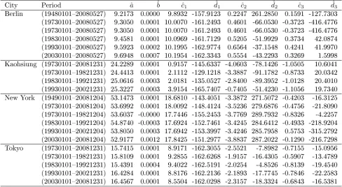
We rst check seasonality, intertemporal correlation, and seasonal variation. Table 1 provides the coecients of the Fourier truncated seasonal function (3) for some cities for dierent time periods. The coecient a can be seen as the average temperature, the coecient b as an
City Period ˆa ˆb ˆc1 dˆ1 ˆc2 dˆ2 ˆc3 dˆ3
Berlin (1948010120080527) 9.2173 0.0000 9.8932 -157.9123 0.2247 261.2850 0.1591 -127.7303
(1973010120080527) 9.3050 0.0001 10.0070 -161.2493 0.4601 -66.0530 -0.3723 -416.4776 (1973010120080527) 9.3050 0.0001 10.0070 -161.2493 0.4601 -66.0530 -0.3723 -416.4776
(1983010120080527) 9.4581 0.0001 10.0969 -161.7129 0.5205 -51.9929 0.3734 42.0874
(1993010120080527) 9.5923 0.0002 10.1995 -162.9774 0.6564 -37.1548 0.4241 41.9970
(2003010120080527) 9.6948 0.0007 10.1954 -162.3343 0.5554 -43.2293 0.3269 1.5998
Kaohsiung (1973010120081231) 24.2289 0.0001 0.9157 -145.6337 -4.0603 -78.1426 -1.0505 10.6041
(1973010119821231) 24.4413 0.0001 2.1112 -129.1218 -3.3887 -91.1782 -0.8733 20.0342
(1983010119921231) 25.0616 0.0003 2.0181 -135.0527 -2.8400 -89.3952 -1.0128 20.4010
(1993010120021231) 25.3227 0.0003 3.9154 -165.7407 -0.7405 -51.4230 -1.1056 19.7340
New York (1949010120081204) 53.1473 0.0001 18.6810 -143.4051 -3.3872 271.5072 -0.4203 -16.3125 (1973010120081204) 53.6992 0.0001 18.0092 -148.4124 -3.5236 279.6876 -0.4756 -21.8090
(1973010119821204) 53.6037 -0.0000 17.7446 -155.2453 -3.7769 289.7932 -0.8326 -4.2257
(1983010119921204) 54.8740 -0.0003 17.6924 -152.7461 -3.4245 284.6412 -0.4933 -218.9204 (1993010120021204) 53.8050 0.0003 17.6942 -153.3997 -3.4246 285.7958 0.5753 -315.2792 (2003010120081204) 52.9177 0.0012 17.8425 -151.2977 -3.8837 287.2022 -0.1290 -216.7298
Tokyo (1973010120081231) 15.7415 0.0001 8.9171 -162.3055 -2.5521 -7.8982 -0.7155 -15.0956
(1973010119821231) 15.8109 0.0001 9.2855 -162.6268 -1.9157 -16.4305 -0.5907 -13.4789
(1983010119921231) 15.4391 0.0004 9.4022 -162.5191 -2.0254 -4.8526 -0.8139 -19.4540
[image:15.595.63.552.79.347.2](1993010120021231) 16.4284 0.0001 8.8176 -162.2136 -2.1893 -17.7745 -0.7846 -22.2583 (2003010120081231) 16.4567 0.0001 8.5504 -162.0298 -2.3157 -18.3324 -0.6843 -16.5381
Table 1: Seasonality estimatesΛˆtof daily average temperature. All coecients are non-zero
at 1% signicance level.
estimation is done in a window length of 10 years. In the sense of capturing volatility peak seasons, the right panel of Figure 3 visualises the power of capturing volatility peak seasons by the seasonal local smoother (5) using the quartic kernel over the estimates modeled under Fourier truncated series (3).
After removing the local linear seasonal mean (5) from the daily average temperatures (Xt =
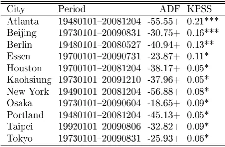
Tt−Λt,LLR), we check that Xt is a stationary process with the Augmented Dickey-Fuller
(ADF) and the KPSS tests. The analysis of the partial autocorrelations and the Akaike Information criterion (AIC) suggest that an AR(3) model ts the temperature evolution
well. Table 2 presents the results of the stationarity tests. The temperature data and the smoothed seasonal functions are plotted on the left panel in Figure 3. To show the pattern of the squared residuals after seasonal and intertemporal tting (εˆ2
t,j), we plot the averaged
20060101 20070101 20080501 −15
−10 −5 0 5 10 15 20 25 30
Temperature in °C −Berlin
Time Jan Feb Mar Apr May Jun Jul Aug Sep Oct Nov Dec 0
2 4 6 8 10 12
Time
Seasonal Variance −Berlin
20060101 20070101 20080501 20
30 40 50 60 70 80 90
Temperature in °C −New−York
Time Jan Feb Mar Apr May Jun Jul Aug Sep Oct Nov Dec 0
10 20 30 40 50 60 70
Time
Seasonal Variance −New−York
200601010 20070101 20080501 5
10 15 20 25 30
Temperature in °C −Tokyo
Time
Jan Feb Mar Apr May Jun Jul Aug Sep Oct Nov Dec 1
2 3 4 5 6 7 8 9
Time
[image:16.595.114.474.164.580.2]Seasonal Variance −Tokyo
City Period ADF KPSS
Atlanta 1948010120081204 -55.55+ 0.21***
Beijing 1973010120090831 -30.75+ 0.16***
Berlin 1948010120080527 -40.94+ 0.13**
Essen 1970010120090731 -23.87+ 0.11*
Houston 1970010120081204 -38.17+ 0.05*
Kaohsiung 1973010120091210 -37.96+ 0.05* New York 1949010120081204 -56.88+ 0.08*
Osaka 1973010120090604 -18.65+ 0.09*
Portland 1948010120081204 -45.13+ 0.05*
Taipei 1992010120090806 -32.82+ 0.09*
[image:17.595.182.412.76.226.2]Tokyo 1973010120090831 -25.93+ 0.06*
Table 2: ADF and KPSS-Statistics for the detrended daily average temperature time series for dierent cities. '+' corresponds to a signicance level of 0.01 for ADF test, and '*', '**' and '***' corresponds to signicance levels of 0.1, 0.05 and 0.01 respectively for KPSS test.
and the xed bandwidth local linear method. Furthermore, we check the normality of the nal residuals and present the results in the Supplementary Material Tables 13 (see there the Fourier method). All seasonal variance estimators lead to residuals that are far from being normally distributed. These facts are of course not an ideal platform for risk neutral pricing (based on standard stochastic nancial models). The heavytailedness, as seen in Figure 1, may be attributed to an unsatisfactory extraction of the heteroscedasticity (or mean) function. As a solution we employ a localisation scheme.
The adjustment in the smoothing parameter h will provide the localisation in time. The
bandwidth sequences are selected from six candidates: (1,2,3,4,5,6,7), (1,2,3,5,7,10,13),
(3,5,7,9,11,13,15),(3,5,8,12,17,23,30),(5,7,10,14,19,25,32), and(7,9,11,14,17,10,24).
These candidates are chosen according to the lowest AndersonDarling (AD) statistic. The best candidate for the bandwidth sequence is the one which yields a residual distribution clos-est to the normal one. Smoothing the selected bandwidths gives another adaptive clos-estimator, implemented, but not discussed here, due to space limitations.
The Critical Values as calibrated from (12) and (13) are given in Figure 4. The left hand side provides Critical Values simulated from a sample of 10000 observations for a quartic
signicance level α. The Critical Values for dierent bandwidth sequences are displayed on
the right hand side of Figure 4. The Critical Values, as one observes, are relatively robust to the choice of r and α.
5 10 15 20 25 30
0.00
0.10
0.20
0.30
0 5 10 15 20 25 30
0.00
0.10
0.20
[image:18.595.115.479.153.304.2]0.30
Figure 4: Simulated Critical Values for likelihood of seasonal variance (9) with θ∗ = 1,
r = 0.5, number of simulation runs = 10000 with α= 0.3 (dotted), 0.5(dashed), 0.7 (solid)
for the bandwidth sequence (3,5,8,12,17,23,30) on the left plot and with α = 0.3 and for
sequences (3,5,7,9,11,13,15) (solid), (3,5,8,12,17,23,30) (dashed), (5,7,10,14,19,25,32)
(dotted), and (7,9,11,14,17,10,24) (dot-dashed) on the right plot.
A one year period is considered in the rst place for demonstration purposes, while later we show how the results change with dierent time periods. Figures 5, 6, 7, and 8 present the general results for the dierent cities under dierent adaptive localising schemes for seasonal mean (Me) and seasonal variance (Va): with xed bandwidth curve (), adaptive bandwidth curve (ad), and truncated Fourier (Fourier) for dierent time intervals. The seasonal mean is estimated jointly over the years, using α= 0.7 and power level r = 0.5.
●●●●●●●
●●
●●
●●
●●●●●
●●
●
●
● ●●●
●●●●
●●
●●●
●
●●
● ●●●●●●●●
●●● ●●●●●●●●●●●●●●●●●●●●●
● ●●●●●●●●●
● ●●●
●●●●●●
●●
●●
●●●●●●●●●●●●●●●●●●●●●●●
●●● ●●●●●●●●●●●●●●●●●●●●●●●●●●●●●●●●●●
●●
●●●●●
●●● ●●●●●●●●●●●●●●
●●
●●●●
● ●●●●●●●●
●●● ●●●
●●
●●●●●●●●●●●●●●●●●●●●●●●●●●●
●●
●●●●●●●●●
●●
●●
●●
●●●●●
● ●●●●●●●●●●●●●●●●●●●●●●●●●●●●●●●●●●●●
●●● ●●●●
●●●●● ●●●●
●
●●
● ●
● ●●●●●●●●
●●● ●●●
●●
●●●●●●●●
● ●●●
●●● ●●●●●●●●●●●●●●●●●●●
● ●●●
●
Index
bandwidth
8
10
12
14
16
0 100 200 300
−10
0
10
20
30
mean
(a) Mean, 2007
● ●
●
●●
● ●●●
● ●●●
●●
●●● ●
●
●●●
●●
●
●●●●●● ● ●
●
●●● ● ●
●
●●
● ●●●
● ●
●●
●
●●
●●
●●●
●
●●
● ●●●●●
●●
●●●
●
● ●●●●
●●●●
●●●●● ●●●●●●
●●●● ●●●●●●
●●●●●●● ●●●
●●
●●
●●
●
●
●●●● ●●●●
●●
●●●
●
●●
●●
●●●●●
●
● ●
●●
●
●●
●●
●
●
●
● ● ● ●●●
●●● ●●●●●●●●●●●●●●●●●
●●
●●●●●●●
●●● ●●●
●●●●● ●●●
●●●● ●●●●
●●●●●●
●●
●●●● ●●●●
●●
●●● ●
●●●●●●●●●●●
●●
● ● ●
●
●●
●
●●
●●●●●●●●●●●●●●●●●●●
●●
●●
●
●●
● ●●●●●●
●●● ●●●●●●
●●●●●
●●
●●● ●●●●
●●●●●●
● ●●●
●●●●
●●
●●●● ●●●●
●●●●● ●●●●●●
●●●
●
●●
●●
●●●
●●
●●
Index
bandwidth
8
10
14
18
0 100 200 300
0
10
20
30
v
ar
iance
0
10
20
30
● ● ● ● ● ● ● ● ● ●
(b) Variance, 2007
●●●●●●
●●● ●●●
●●●●●●●●
●●
●
●●
●●●●●●●● ● ●
●●
●●● ●●●●●●●●●●●
●
●●
●
●●
●●
●●●●●
●●● ● ●
●
●●● ● ●
●
●●●● ● ●
●
●
●●●
●●
●
●●
●●
●●● ● ●
●
●●●
●●
●
●●●● ●
●●●●●●●●●●●
●●
●●●●● ●
●●
●●
● ●
●
●●●● ●●●●●●●●●●●●●
●
●●
●●● ●●●●
●●●
●●●● ●●●●●●●●
●●● ●●●●●●
●●● ●●●
●●●● ●●●●●●●●●●●●
●●●●●●●
●●
●●●●●●● ●●●●
●●●●
●●
●●●●● ●●●●●●●●●●●●●●●●●●●●
●●●●
●●
●●●●
●●
●●● ●
●●●●●● ●●●●●●●
●●●●●
●●
●●●●●●
●●
●●●● ●●●
●●
●●●●●
●●●
●●●● ●●●
●●
●●
● ●●●●
●
●●●●●●●●●●●●●●●●
●●● ● ●
●
●●
●●
Index
bandwidth
10
12
14
16
0 100 200 300
15
20
25
30
mean
(a) Mean, 2008
●
● ● ●
●●
●●●
●●
● ● ●
●●
●●●●●
●●●
●●
●●
●●●●●●
●●
●●●●
●●
●
●
● ● ●
●●●●●● ●
●
● ●
●
●●● ●
●
●
●●
●●
●●
● ● ●
● ●●●●●
●
● ● ●●●
●●●●●●
● ● ●
●
●●
●●
●●
● ●●●
●●● ●
●
●●
● ● ●
●●●●● ●
●●● ●●●
● ●
●●●●
●●
●●
●●
● ●
● ● ●●●
●
● ●●●
●
●●
● ●●●●
●●
●
●●
●●
●●
●●● ● ●
●●●●
●●
●
●●● ●
● ● ●
● ● ●●●
●●
●
●
● ●●●●●●●●●
●●●●●●●●●●
● ● ●●●●
●●● ●
●
●●
●●
●●
●●
●●●●●●
●●●●
●●
●●● ●●●
●●●●
●●
●●● ●
●
●
●●
●●
●●●●●● ●
●
● ● ●
● ●●●
●●●
●●
●●
●●
●●●●●
●●
●●●●
● ●
●●●● ●
●●● ●●●●●
● ●●●
●●
●
●●●●
●●
●●●
●●●
●●
●
●●
●
●●●
●●
●
●
●●
●
●●
●●
● ●
●●●● ●
Index
bandwidth
5
6
7
8
9
10
0 100 200 300
0
2
4
6
8
12
v
ar
iance
0
2
4
6
8
12 ● ● ● ● ● ● ● ● ● ●
(b) Variance, 2008
●●●●●● ●●●
●
●●
●●
●
● ●
●●
●●
●●●
●●● ●●●
●●●●●●
●●
●●●
●
●●
●●
●●
●●●●●●●●●
●●●●●●● ●●●
●●
●●●
●●
●
●●
● ●●●●
●●●●●
●●●●● ●●●
●●●●● ●●●
●●●●●● ●●●
●●●●● ●●●●●
●●●● ●●●●●●●●●●●●●●
●●● ●●●
●●●●●● ●●●●
●●●●●● ●●●●●●
●●
●●●●●●●●●●●●●●●●●●●●●●●●●●
●●●●
●●
●●●●●● ●●●
●●●●●● ●●●●
●●●●● ●●●●●
●●●● ●●●●●●●●●●●●●●●●●●●
●●
●●●●●●●●●●●●●●●●●●●●●●●●●●●●●●
●●
●●
●●● ●●●
●●●●
●●
●●
●●
●
●●
●
●●
●●●●●●●●● ●
●●
●●
●●
●●
●●
●●● ● ●
●●
●●●
●●
●●
●●●● ●●●●●●●
●●● ●●●●●
Index
bandwidth
10
12
14
16
18
0 100 200 300
0
10
20
30
mean
(a) Mean, 2007
●●
● ●●●●●
●
●●
● ●
●●● ●●●●●
●
●●
● ●●●●●●●●●
● ●●●
●●
●●●●
●
●●
●●● ●
●
●
●●
●●●●●●●●
●
●●
●●
●●
●●●●●
●●
●●
● ●
●
● ●●●
●●
● ●
●●●● ●●●●●●
●●
●●●●
●
●●
●●
●●●●●●●
●●
●●
●●
●●
●●●
●●
●●●●
●
● ● ●●●●●
●●
●●●
●●● ●●●
●●● ●●●●●●●●●●●●●●●●
●●
●
●
● ● ●
●●
● ●●●●●
●●●●
● ● ●
●●●● ●
● ● ●●●●
●●● ●●●
●●● ●
●●
●●●
● ●●●
●●
●●
●
●
● ● ●●●●●●●●●●●
●●
●
●●
●●●●
●●
●
●●●●● ●●●
●●
●●
●
● ●●●●●●●●●
●●●
●●
●●
●●●●●●●●●
●●
●●●
● ●●●●●●●●●●●●●●●●●●●
● ●●●●●●●
●●●● ●●●●
●●
●
●●
● ● ●
●
●●
●
● ● ●●●●●●●●●●●●●●
●
Index
bandwidth
6
8
10
14
0 100 200 300
0
10
20
30
40
v
ar
iance
0
10
20
30
40
● ● ● ● ● ● ● ● ● ●
(b) Variance, 2007
●●●●●●●●●●●●●●●●●●●●●●●●●●●●●●●●●●●●●●●●●●●
● ●●●●●●●●●●
● ●●●●●●●
● ●●●●●●●●●●●●●●●●●●●●●●●●●●
● ●●●●●●●●●●●●
● ●●●●●●
●●
●●●●●●●●●●●●●●●●
● ●●●●●●●
● ●
●
●●●●●●●●●●●●●●●●●●●●●●●●●●●●●●●●●●●●●●●●●●●●●●●●●●●●●●●●●●●●●●●●●●●●●●●
● ●●●●●●●●●●●●●●●●●●
● ●●●●
● ●●●●●●●●●●●
●
●●
● ●●●●
● ●●●●●●●●●●●●●●●
● ●
● ●●●●●●●●●●●●●●●●●●●●●●●●●
●
●●
●
●●●●●●●●●●●●●●●●●●●●●●●●●●●●●●●●●●●●●●●●●●●●●●●●●●●●●●●●●●●●
● ●●●
Index
bandwidth
5.0
5.5
6.0
6.5
7.0
0 100 200 300
5
10
20
30
mean
(a) Mean, 2008
●
●
● ● ●●●
●●●●●
●
● ●●●●●●●●
● ●●●●●●
● ●●●●
●●●● ●●●●
●
● ● ●
●●● ●
●●
●●
●●
●
● ●
●●
●●● ●●●
●●
● ●
● ● ●●●●●●●
●
●●
●●
●●●
●●● ●●●●
●
●●●
● ●●●●●●●
●●
●●
●
● ● ●
●●
●
● ●●●
●●●●●●
●●
●●● ●
●●
● ● ●
●
●
●●
●●
●●
●●●●●
●●●●●
●●
●
●●
●●
●●●●●●●●
●●● ●●●●●
●●
●●●●●●●●
●●
●
●●
●
● ● ●
●
●
●●
●●
●●
●●●● ●
●●
●
●●
●●
●
●●
●●● ●
●●
●●
●●
● ●●●
●●●
● ●●●
●●●●
●●● ●●●●●
●●
●●●●
●●
●●●
● ●
●
●●
●●
●●
●●
●●
●●
●●●●●●
●●
●
●●
●
●●
●●
● ● ●
●●●●●●●●●● ●
●●●
● ● ●●●●
●●● ●●●●●
●●●●●●
●●
●●● ●
●
● ●
●●●●●●●●●
●●● ●●●
● ●
●●●● ●
Index
bandwidth
6
8
10
14
0 100 200 300
0
5
10
20
v
ar
iance
0
5
10
20
● ● ● ● ● ● ● ● ● ●
(b) Variance, 2008
Method Explanation
JoMe adMe adVa Jointly estimated mean, adaptive bandwidth mean adaptive bandwidth variance
JoMe Me Va Jointly estimated mean, xed bandwidth mean xed bandwidth variance
SeMe adMe adVa Separately estimated mean, adaptive bandwidth mean adaptive bandwidth variance
SeMe Me Va Separately estimated mean, xed bandwidth mean xed bandwidth variance
Locave Aggregated approach with average of yearly empirical variance as the target
Locsep Aggregated approach with each year's empirical variance as the target
Locmax The optimal between Locave and Locsep (minimize the p value)
Fourier Method with Fourier series tting for mean and variance
CD Method adopted by Campbell and Diebold (2005)
Table 3: Summary of methods
to ten dots of the upper and lower tails of the QQ-plots of square residuals respectively (see Figure 9 for the Berlin results). The top plots of Figures 58 show the mean case. Unlike the seasonal variance function, we do not observe a big variation of smoothness in the mean function. One can see that in all cities, the bandwidths vary over the yearly cycle with a slight degree of non homogeneity for Kaoshiung.
An approach to cope with the non normality brought in by more observations is to estimate mean functions year by year (SeMe), and then aggregate the residuals for variance estimation. We therefore estimate the joint/separate seasonal mean (JoMe/SeMe) and seasonal variance (Va) curves with a xed bandwidth curve () and an adaptive bandwidth curve (ad). (A summary of the estimation methods can be found in Table 3.) The average over years acts as a smoother when we consider more years. The estimated AR(L) parameters for
dierent cities using a joint/separate mean (JoMe/SeMe) with dierent bandwidth curves are illustrated in Table 4. The results again show that an AR(3) ts the stylised facts of
temperature well.
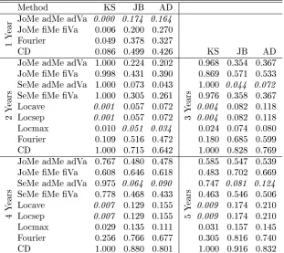
KolmogorovSmirnov (KS), JarquesBera (JB) and AD normality tests are taken to test the normality of the corrected residuals (after seasonal mean and variance). For each city, a rejection at 0.05 level is counted as 1 (else 0). The rejection rates over all the cities
under dierent estimation techniques are displayed in Table 5. The results compare dierent periods (1−5 years) for the robustness of our methods. (Considering data histories longer