Optimization of a log wood boiler through CFD simulation methods

City, University of London Institutional Repository

Citation

:

Athanasios, N., Nikolopoulos, N., Nikolaos, M., Panagiotis, G. and Kakaras, E.

(2015). Optimization of a log wood boiler through CFD simulation methods. Fuel Processing

Technology, 137, pp. 75-92. doi: 10.1016/j.fuproc.2015.04.010

This is the accepted version of the paper.

This version of the publication may differ from the final published

version.

Permanent repository link:

http://openaccess.city.ac.uk/8700/

Link to published version

:

http://dx.doi.org/10.1016/j.fuproc.2015.04.010

Copyright and reuse:

City Research Online aims to make research

outputs of City, University of London available to a wider audience.

Copyright and Moral Rights remain with the author(s) and/or copyright

holders. URLs from City Research Online may be freely distributed and

linked to.

Nomenclature and units

CFD

computational fluid dynamics

LHV

lower heating value

LPG

liquefied petroleum gas

MDF

medium density fiber

RANS

Optimization of a log wood boiler through CFD simulation methods

Nesiadis Athanasiosa

Nikolopoulos Nikolaosa, b, ⁎

[email protected]

Margaritis Nikolaosa, b

Grammelis Panagiotisa

Emmanuel Kakarasa

a_{Centre for Research & Technology Hellas/Chemical Process and Energy Resources Institute (CERTH/CPERI), 4th km. N.R. Ptolemais-Mpodosakeio, GR-50200, Ptolemais, Greece}

b_{Clean EnergyLtd, 4th km N.R. Ptolemais-Bodosakeio, Kozani, Greece, GR-50200}

⁎_{Corresponding author at: 52, Egialias str.,GR-15235, Maroussi, Greece.}

Abstract

This paper describes the steady-state modelling modeling and simulation of a wood log fired boiler. It is designed and manufactured by THERMODYNAMIKI S.A. (KOMBI), a company based on Northern Greece. Its nominal fuel power isaround to 32 kW and its efficiency is close to 75%.A specific operating case, selected and experimentally investigated by the manufacturer, is examined. Due to the highly transient and complex nature of wood log combustion, an ad-hoc model has been developed. Its main characteristic is the fuel division into three components: water vapor, volatiles and fixed char. The latter is considered to form a layer, which is treated as a porous medium thus forming a volumetric source zone adjacent to the firebed area. Volatiles and water vapor are modelled modeled as volumetric mass sources, whereas a two-step reaction mechanism of the former is considered. The numerical results are compared against corresponding experimental data for the nominal load as far as flue gas characteristics (temperature and species concentration) at the boiler exit, are concerned. Based on the validated model, a proposed optimization pattern of the boiler is undertaken and examined by means of CFD.

Reynolds Averaged Navier Stokes

RTE

radiative transport equation

TGA

thermo-gravimetric analysis

Abbreviations

A

pre-exponential factor (1/s)

C1ε

turbulence model constant, (1.44)

C2ε

turbulence model constant, (1.92)

C3ε

turbulence model constant,

CIN

inertia loss coefficient (1/m)

Cp

heat capacity (J/(kg K))

Cµ

turbulence model constant, (0.09)

D

diameter (m)

E

total energy (J)

E’′

activation energy (J/k mol)

external body forces (volumetric), (N/m3₎

gravitational acceleration (m/s2₎

Gb

turbulence kinetic energy generation due to buoyancy (kg/(ms3₎₎

Gk

turbulence kinetic energy generation due to velocity gradients (kg/(ms3₎₎

H

sensible enthalpy (J/kg)

h0

formation enthalpy (J/kg)

H

total enthalpy (J/kg)

I

radiation intensity (W/m2₎

Ji

species diffusion flux (kg/(m2 _s))

K

turbulent kinetic energy (m2_/s2₎

kd

devolatilization kinetic rate (kg s-− 1 _m-− 2_(Nm-− 2₎-− 1₎

L

bed depth (m)

ṁ

mass flow rate (kg/s)

m’′

mass per mass fuel (kg/kg)

Mw

molecular weight (kg/k mol)

N

P

pressure (N/m2₎

position vector

R

universal gas constant, (8314 J/(k mol K))

ℜ

net rate of species production (volumetric) (kg/(m3 _s))

direction vector

scattering direction vector

S

Path length (m)

Sh

heat sources (volumetric)(W/m3₎

Si

species sources (volumetric) (kg/(m3 _s))

Sk

turbulence kinetic energy sources (kg/(ms3₎₎

Sm

mass sources (volumetric) (kg/(m3 _s))

Sε

turbulent dissipation rate sources (kg/(ms4₎₎

t

time (s)

T

temperature (K)

velocity (m/s)

x

distance (m)

Y

species mass fraction (-−)

YM

contribution of the fluctuating dilatation to the turbulent dissipation rate (kg/(ms3₎₎

Subscripts

ar

as received

db

dry basis

daf

dry ash free

cell

cell

d

devolatilization

eff

effective

f

fluid (continuous phase)

fuel

fuel

L

air

LoT

dry stoichiometric air

dry air r reaction s solid p particle t turbulent Greek letters α

absorption coefficient (1/m)

αp

medium permeability (m2₎

γ

porosity

ε

turbulent kinetic energy dissipation rate (m2_/s3₎

ε_v

void fraction (-−)

κ

thermal conductivity (W/(m K))

λ

air to fuel ratio (-−)

µ

dynamic viscosity (kg/(ms))

ρ

density (kg/m3₎

σ

Stefan-–Boltzmann constant, (5.67 x × 108 _W/(m2 _K4₎₎

σk

turbulent kinetic energy Prandtl number, (1.0)

scattering coefficient (1/m)

σε

turbulent dissipation rate Prandtl number, (1.3)

stress tensor (kg/ms2₎

χ

mass per mass air (kg/kg)

φ

scalar quantity

Φ

Radiation phase function

Ω’′

solid angle (sr)

1 Introduction

Nowadays, wood is commonly used for space heating and power generation in the developed countries, whereas it remains a primary energy source in domestic and industrial environments in many developing countries. Its use as a fuel is considered to be carbon neutral, since it can be combined with a sustainable model of cultivation and consumption. For this reason wood is included in the renewable energy sources and particularly in the “biomass and wastes” category. The use of the latter faced a rapid expansion in the EU27, up to 139%, between 1990 and 2008 [1], as a part of the strategy to reduce greenhouse gas emissions. In 2010 wood and waste was were the leading source of renewable energy accounting for 49% of the renewable consumption, while it contributed 4.8% to the total gross inland energy consumption of European Union [2]. In Greece these values were 38% and 2.9% respectively, whereas noteworthy is the fact that in 2011 fuelwood accounted for 72% of the country’'s roundwood production [2]. Apart from the near zero CO2 emissions, another advantage of wood compared to fossil fuels is its lower sulfur and nitrogen concentration resulting in reduced SOX

and NOX emissions [3]. However, wood combustion should be carefully treated since insufficient burning results in harmful particle and CO emissions.

Wood combustion characteristics have been the subject of several studies. Anca Couce et al. [4] determined a kinetic model of pine wood smouldering smoldering by thermo-gravimetric analysis (TGA), which includes five components, i.e. three wood pseudo-components, char and ash. The former devolatilize through pyrolysis or oxidation, depending on oxygen concentration, while char oxidizes and produces ash. The model validity was confirmed against other well-established models. Yorulamz and Atimtay [5] investigated the combustion mechanisms of treated waste wood samples (MDF, polywood and particleboard) using TGA and compared them to the behavior of untreated pine. Based on their TGA results they determined three thermal degradation mechanisms. A first one is owed to moisture and highly volatile matters, a second one during which the removal and oxidation of volatiles take place and a third region characterized by the oxidation of the char remaining. In all cases, the dominant oxidation mechanisms were determined. Amutio et al. [6] studied the pyrolysis behavior and kinetics of forest shrub wastes. Three independent and parallel reaction models corresponding to the decomposition of hemicellulose, cellulose and lignin were utilized for describing the samples degradation. Their study concluded that the forest wastes valorization by pyrolysis is possible. Skodras et al. [7] examined the pyrolysis and combustion characteristics of 10 biomass and waste materials. A model involving three or four parallel reactions was employed for simulating the devolatilization process and evaluating the kinetic parameters. The effect of heating rate was also investigated. Finally, Di Blasi [8] in an extensive review summarized the latest advances in modeling chemical and biomass processes of wood and biomass pyrolysis. This survey is not restricted only in chemical kinetics, but also includes transport models of biomass particle pyrolysis and models of pyrolysis reactors. The fixed-bed reactors reactor models are based on the assumption that the bed forms a continuum porous solid, but generally they are empirical and valid only in specific experimental conditions.

interaction with the gas phase in biomass packed beds. Drying, devolatilization and char oxidation and gasification constitute the introduced combustion scheme. Their model was tested in the case of an experimental burner with satisfactory results. Zhang et al. [12] presented an experimental and numerical investigation of the performance of a wood chip fired residential boiler. The applied numerical model consisted of two sub-models: one for the burning bed and one for the freeboard flow, which interacted with each other. They focused mainly on the flue gas emissions and explored the effect of various boiler aspects on them.

The numerical simulation of an 18 kW domestic boiler was performed by Collazo et al. [13]. In contrast to the previously mentioned studies, a simplified method was developed assuming that the particles in the bed are in thermal equilibrium with the gaseous phase. Another simplification is the constant temperature consideration for calculating the pyrolysis and char oxidation products. The comparison of numerical results with experimental data showed an acceptable level of accuracy, but the model applicability is limited in cases where the gases residence time is no longer than the time required for their reaction, i.e. when the bed is type of a stirred reactor. Another simplified method for simulating fixed-bed pellet boilers was introduced by Chaney et al. [14]. Its main feature is the fact that fixed bed is not modelled modeled as a porous zone, but as discrete devolatilization zones within the bed region. The devolatilization rate in its cell is configured so as to ensure correct mass and energy balance. In the same zones the char combustion takes place – — its rate is controlled by the desired power output and the fuel mass flow. The computational results proved to be quite promising. Finally, Shiehnejadhesar et al. [15] developed an empirical fixed bed combustion model. It consists of 1D profiles of the fuel components along the grate, parameters describing the fuel components conversion to flue gas and governing the local composition of the latter and finally calculation of the local energy and mass profiles. It is combined with an Eulerian treatment of the gaseous phase and of the corresponding volumetric reactions. This method was utilized for the design optimization of an 180 kW biomass furnace concerning the minimization of CO emissions with satisfactory results. The same fixed bed model was adapted in order to derive time-dependent profiles of wood log combustion and was applied in a wood log fired stove optimization study [16]. In this case, the fuel was divided into water vapor, fixed char and volatiles and the latter were released from the outer layer of the logs. The numerical results were tested successfully against experimental data. The optimized design combined considerably reduced CO emissions and more than 10% thermal efficiency increase. The same formulation was later used for the development and optimization of several small-scale biomass furnaces and stoves [17]. Reduction of the NOX emissions and fine particle formation was of particular interest in all cases.

To relate this work with similar referencedreferences, the published papers dealing with the numerical investigation of small-scale domestic boilers are very few. Compared to the work of other researchers, the current study does not focus only on the CFD investigation of a boiler, but also includes a design optimization concept which appears to improve the boiler operational characteristics. In that sense, the character of this work is not purely academic, but may also have an industrial impact.

Moreover, a unique characteristic of the specific boiler under investigation is the utilization of the water-tubes like a scab for the fixed bed formation. This configuration presents several modeling difficulties, since the fixed bed formed is very close to a wall surface of a non-flat geometry.

Another characteristic of this study is the use of a very dense numerical grid (1.1 million elements), specifically being much denser at the vicinity of the heat exchanging surfaces (inflation layers), for such a very small volume, which can be regarded to increase significantly the accuracy of the CFD results. Especially those concerning the induced wall heat flux. Specific results concerning the grid dependency on the predictions are presented in a following section. In similar works, coarser grids of around 217,000 [12] or 700,000 [15] cells have been implemented for the modeling of small-scale boilers (load > 150 kW). Last but not least, the use of porous media approaches for the modelling modeling of the fixed bed is a feature which can be found in several other works, [10,11,13,16,17]. However, a detailed literature review on available model approaches for fixed beds [14] confirms that this approach is not commonly used in such systems.

2 Methodology and scope

The successful numerical simulation of the boiler steady-state operation is defined as the first task. The tool used for CFD simulations is the commercial software ANSYS Fluent. The parametric geometry software ANSYS Design Modeler and ANSYS Meshing software are used for the boiler geometry reconstruction and numerical grid generation respectively.

In order to validate the numerical results, experimental measurements of the flue gas composition and temperature, as well as of the inlet air properties are performed by the boiler manufacturer. A portable combustion analyzer is used for the measurement, which has also the ability to estimate the boiler efficiency and the draught of the air flow. Inlet and outlet temperatures of the water are also reported. Fuel (wood) chemical analysis is carried out by CERTH. All these available data are used in order to simulate as accurately as possible the fuel combustion and the subsequent heat transfer phenomena taking place in the boiler interior.

Generally such small scale boilers undergo a three step sequence of fuel combustion (heat-up, constant load or stationary operation and cool-down period). Nevertheless, the principal scope of this work is to build a steady-state numerical model capable of predicting the boiler behavior during its constant load operation, assuming that the fuel and oxidizing medium flow rates along with their corresponding compositions are kept constant. In that light and during that period of time, the manufacturer was only capable of monitoring the key-values at the boiler exit only at specific time instants with a portable gas analyzer. Unfortunately, the measurement equipment used is not linked with a data logging system in order to provide a series of real time measurements. Given this restriction, it is decided to use experimental data for the flue gas exiting the boiler collected at four equal spaced 5 minutesmin time instants.

Finally as well referenced in similar papers conducting that kind of research, during the constant load boiler operation, the flue gas exit values change in time with a deviation less than 1-–1.5% [12]. This deviation is valid for the CO2 and

boiler thermal efficiency and/or the emission reduction are is the expected features of the new design. Since any alterations entail financial cost and/or constructional difficulties, the final decision upon the applied changes depends on the manufacturer. Finally, it should be stated, that the model is capable, with this steady-state approach, of predicting any time instant boiler operation, with the prerequisite that all available input data are available

2.1 Simulation of the boiler

The boiler under consideration is the KOMBI kn 30/50 model. It is a wood fired boiler, which has the ability to burn various forms of solid fuels such as firewood and charcoal. It can also be converted into oil or LPG burning boiler, while maintaining high efficiency. A general view of the boiler is displayed in Fig. 1.

The boiler is manufactured from high quality steel St-37.2.It is insulated with a 3 cm layer of high density fiberglass and externally lined with pre-painted steel sheets. The fuel is supplied through a large opening door (marked with (a) in Fig. 1), placed at the upper front side of the boiler. There is only one air inlet, a small door of rectangular cross-section placed at the lower front side (marked with (b) in Fig. 1). The air flow is based on the mechanism of natural convection, as there is no ventilator. Both front doors are made of vermiculite and their thickness is 6 cm.

The management and conservation of the solid fuel is carried out by a mechanical thermostat. The combustion chamber design permits a constant 24 hoursh operation with low fuel feeding requirements (3-–4 times a day). Its grid consists of 6 water tubes made of seamless steel. The boiler main technical characteristics are summarized in Table 1.

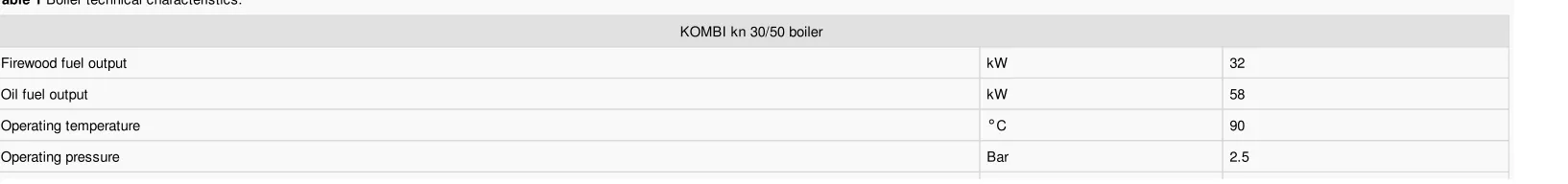
Table1 Boiler technical characteristics.

KOMBI kn 30/50 boiler

Firewood fuel output kW 32

Oil fuel output kW 58

Operating temperature

°

Operating pressure Bar 2.5

Water capacity lt 110

Main dimensions

Height mm 1270

Width mm 540

Length mm 820

Weight kg 242

As it is presented in Fig. 2, the water chamber almost encircles the whole combustion zone. The right, left, top and back sides of the later latter are in full contact with water. A small part of the front side also contributes to the heat transfer, as a tube of rectangular cross-section is placed between the two doors. Water circulation between the left and the right side of the boiler is achieved by the front-placed tube and the 6 water tubes. After the combustion chamber, the flue gases enter a small transition zone and finally reach the 6 elliptical shaped flue-tubes. Their surface is also in contact with water, boosting the boiler efficiency. A conjoiner part connects these 6 tubes with a cylindrical chimney.

2.1.1 Basic equations

The flow is calculated in an Eulerian frame and cell elements are used to discretize the computational domain. In order to simulate the dynamic part of the flow the Reynolds Averaged Navier Stokes (RANS) equations are solved. The continuity expression is given by Eq.(1):

In this equation, mass sources are encountered to take into account the additional sources/sinks owed to the heterogeneous reactions taking place. The conservation of momentum is described by Eq.(2).

The deviatoric stress tensor included in the above equation is given by the following form:

The effective viscosity µeff used in Eq.(3), is defined as the sum of the laminar and the turbulent viscosity:

For simulating the effect of turbulence on the fluid flow, the standard k-εturbulence model is applied. It is the most popular model, since it combines robustness, computational economy and reasonable accuracy. It is based on the isotropic turbulence assumption and its main feature is the computation of two transport equations, i.e.one for the turbulent kinetic energy k (Eq.(5)) and another for the corresponding dissipation rate ε (Eq.(6)).

Close to wall boundaries the standard wall functions, based on the law-of-the-wall, are used. The turbulent viscosity which appears in Eqs.(4), (5) and (6) is computed as stated by Eq.(7).

For calculating the local concentrations of the species included in the boiler modeling (i.e. O2, N2, H2O, CO, CO2 and volatiles) a transport equation of the following form is considered for each one of them:

In order to solve the temperature field of the computational domain the following form of the energy equation is solved,

The pressure work and kinetic energy terms are considered to be negligible and are not taken into account in the energy balance. The energy source term Sh represents mainly the energy source due to chemical reactions and depends on the associated

volumetric rate of creation ℜj of species j:

Radiation is an important aspect of the heat transfer that takes place in a boiler. Due to the small dimensions of the latter, the Discrete Ordinates Ordinate (DO) radiation model is utilized in order to simulate such effects. Its main feature is the solution of a radiative transfer equation (RTE) for a finite number of discrete solid angles. The expression of RTE is the following,

The above equation is a transport equation of radiational intensity in the sector of solid angleΩ’′.The value of radiation intensity depends on the position vector and the direction vector , which is associated with the particular solid angle. The number of transport equations solved is equal to the number of the solid angles (or equally of the directions ), which in this case are set equal to 4 per octant.

For the pressure discretization the Presto scheme[18] is used, while for velocity, species, and energy the second order upwind scheme[19]. The pressure-–velocity coupling is calculated on the basis of the standard SIMPLE algorithm[20]. Presto scheme works better for problems with strong body forces (swirl) and high Rayleigh number flows (natural ventilation).

(1)

(2)

(3)

(4)

(5) (6)

(7)

(8)

(9)

(10)

(11)

2.1.2 Fuel properties and combustion

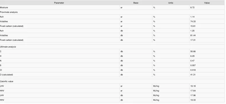
Beech wood is chosen to be the fuel under investigation, which properties were analyzed at the CERTH laboratories. Its main chemical and physical properties are presented in Table2.

Table2 Proximate analysis, ultimate analysis and calorific values of beech wood log.

Parameter Base Units Value

Moisture ar % 8.72

Proximate analysis

Ash ar % 1.14

Volatiles ar % 74.33

Fixed carbon (calculated) ar % 15.81

Ash db % 1.25

Volatiles db % 81.44

Fixed carbon (calculated) db % 17.31

Ultimate analysis

C db % 50.66

H db % 6.29

N db % 0.47

S db % 0.007

Cl db % 0.018

O (calculated) db % 41.31

Calorific value

LHV ar MJ/kg 16.18

HHV ar MJ/kg 17.64

LHV db MJ/kg 17.96

HHV db MJ/kg 19.33

As it is stated previously [16], during the steady state operation of the boiler the fuel (i.e. wood log) is assumed to consist of two separate components:

•Fixed char which forms a fixed bed

•Volatiles and moisture, which are released from an outer layer of the logs

The fixed bed (firebed) is assumed to form a uniform layer, which starts at a height that corresponds to the center of the water tubes. It is assumed to be 7cm thick and covers almost the whole cross-section of the boiler, except from a 1cm wide gap, operating as a buffer zone between the ash layer and the boiler walls. In this layer the fixed char combustion is considered to take place. The heat release corresponds to the complete carbon burnout towards CO2, which is introduced into the computational

height-depended pattern, resembling the real conditions, during which the upper surface of the firebed is experiencing higher temperatures than its bottom.

Furthermore, the firebed is modeled as porous zone. The main flow characteristics of a porous zone are modelled modeled using i) the static pressure drop coefficients and ii) the porosity. Both variables are used to define the resistance of the gas flow experienced by the existing solid ash particles, which in fluid terms is expressed as a drop of the gaseous phase static pressure. A common way to estimate this pressure drop is to use the Ergun equation.

The above expression represents a momentum source term which is added to the standard fluid flow equations. This source term is composed of two parts: i) a viscous term, which is the first term of the right-hand side of Eq.(12) and ii) an inertia loss term, which is the second term of the right-hand side of the same equation. In the framework of the present simulations the value values of these two pressure coefficients are directly defined. The viscous loss coefficient, which is equal to the reverse of the medium permeability aαp is defined as:

The inertia loss coefficient is respectively defined as:

Both coefficient’'s values are considered to be uniform in all directions.

Porosity γ(assumed equal to ε_v) is defined as the volume fraction of fluid within the porous region. This variable affect affects the basic equations, which describe the problem, in various ways. Firstly, it has an effect on the time-derivative terms in all transport equations and the continuity equation. The form of these terms becomes , where ϕ is the scalar quantity. Furthermore, when the porous media modeling is based on the physical velocity of the domain, a formulation followed in the present

case, the porosity must be taken into account in all the terms of scalar equations:

The form of the volume-averaged mass and momentum conservation equations changes respectively:

As far as the energy equation is concerned, the porous medium and the gaseous phase are assumed to be in thermal equilibrium. Thus, a modified form of the Eq.(9) is solved, in which the flux conduction within the porous medium and the thermal inertia of the solid region are included.

In the present case a porosity value of 0.9 is chosen. The corresponding static pressure drop is about 20Pa (Pa order of magnitude).

The wood logs are modeled as volumes that are placed on the ash layer. In the present case two logs of trapezoidal shape are considered, as this shape was proved to be the most suitable to maintain a constant burnout at the log base. Their main dimensions are presented in Fig.3.

(12)

(13)

(14)

(15)

(16) (17)

The inner and larger part of these volumes is assumed to be solid, i.e. air cannot enter in those regions. However, the solid region is surrounded by an outer layer, 2cm thick, which acts as a buffer zone between this region and the ash layer. Its main function is to act as a volumetric source region, from which the volatiles and moisture are released. The required energy for fuel moisture vaporization has been extracted from the total energy input and H2O(g) species sources have been implemented in the

adjacent computational cells at the proximity of the wood geometry.

Wood char combustion takes place on the surface of wood logs in such small-scale boilers. To simulate that either one can assume a thin layer of char applied on the bottom surface of wood logs and then calculate the heterogeneous reactions or just impose the associated mass (CO, CO2 and O2) and energy sink/sources in the adjacent cell volumes. We preferred to use the second approach, since it is simpler and no significant deviation from the real physics problem occurs.

All associated sinks and sources are not considered to be uniform along the wood outer layer but are calculated at each cell as a function of the local calculated rates and corrected proportionally on the basis of each specific cell value, so that the overall integrals can have the exact assumed values. The place of all sinks and sources are is shown in Fig.3.

As it is deduced from Table2, the volatiles contain carbon, hydrogen, oxygen, nitrogen, sulfur and chlorine. However, due to the very low concentrations of the last three species in the fuel and in an attempt to simplify the reactions, it was decided to ignore them from the fuel composition. Thus the chemical formula and the final ultimate analysis of the wood volatiles (Table 3)is are approximated to be the following:

Table3 Ultimate analysis of the wood volatiles.

Parameter Base Units Value

Formula C3.43H7.71O3.19

C daf % 41.21

H daf % 7.77

O daf % 51.03

The volatiles and vapor release is are not uniform along the wood outer layer, but is are controlled by an Arrhenius type single kinetic rate model defined in Eq.(19). The rate value depends on the temperature of each cell of the outer layer, the activation energy value which is equal to E’′d=2.38 x×108 (J/kmol) and a pre-exponential factor. The value of the later latter is a function of the cell volume and its value is updated at every solution iteration in order to conserve a constant value of the relevant mass source

volume integral, equal to 0.001323kg/s.

Fig.3Main dimensions of the wood logs. The ash layer is also visible.

The fuel gaseous phase is homogeneously combusted following a two-step mechanism. At first the volatiles are burnt to form a mixture of CO and H2O. The second step consists of the reaction of CO into CO2. These two reactions and the subsequent

Arrhenius rate coefficients are based on a Westbrook and Dryer 2-step global combustion mechanism for hydrocarbon fuels, summarized in Table4.

Table4 Gas phase reaction schemes and kinetics rates and kinetic rates.

No. Reaction Ar (s-− 1) [18] E

’

′r

1 2.119

×

_×

_⋅

2]1.3

2 CO + 0.5 O2

→

×

×

⋅

As it was reported from the boiler manufacturer, the fuel nominal power related to LHV is around to 32kW, while the corresponding thermal output is measured to be equal toaround22-–24kW. Following an indirect efficiency calculation, based on the measured flue gas composition and temperature resulted in an efficiency equal to around 74.4%.The split of the fuel input between the fixed char (firebed-zone) and the volatile component (main combustion-zone) is configured based on the following constraints:

•The wood ultimate analysis, which in other words sets a the lowest limit for the fixed char component.

•The need to maintain a constant burnout at the log base. This requirement is prescribed not only by the nature of the wood combustion, but is also associated with the flue gas temperature. A contribution of the char component larger than the proximate value has a positive effect on the logs

burnout characteristics.

•The necessity to keep the temperature field within the combustion chamber in reasonable values. A large contribution of the char component results in quite high temperatures.

After several numerical tests on what should be the level of energy provided within the boiler from char combustion, we concluded that a reasonable value should be in the range of 40%. Lower values lead to an unstable flame combustion, thus resulting in the non-reacting gas flow species, since the calculated temperatures were not high enough, while higher values resulted in increased temperature values within the boiler at the proximity of wood logs (>1650 °C), which are not expected in reality. [16,17]

measure a value of around 1200 °C for a an 8kW wood log domestic boiler.

The type of approach, although not so common, is performed by defining user defined sub-routines (UDF) within the CFD code. This code contains the essential details to characterize the solid and gas phase interactions [14,18]. One simple method of doing this is to define the solid biomass as a porous zone, and then write a user-defined function in the CFD describing sources of moisture, volatiles and energy to describe the drying, devolatisation devolatization and char combustion processes respectively. The reliability of the CFD modelling modeling results is, to a large degree a function of the modelling modeling approach adopted and the accuracy of the boundary conditions specified.

The actual char combustion reaction mechanisms within such small scale boilers, are not yet clearly defined owed owing to the complicated in short time physical mechanisms governing its operation. CO prediction is of course an issue and in no case the calculated values should be considered as representative of a real boiler operation. The model applied just follow follows some relevant suggestions referenced in related papers, while for example the reaction of CO with H2O is not taken into consideration.

2.1.3 Mesh details

The grids used for the numerical simulation of the present case were developed on the basis of ANSYS Meshing software. Since a respectable number of CFD tests were identified to be necessary for the definition of the appropriate problem

modelling modeling approach, initially a coarse grid was created. It consists of approximately 240.,000 tetrahedral elements. Nevertheless their quality is high, since their maximum skewness is 0.924 and their minimum orthogonal quality is 0.177 – — both within the acceptable limits (0.94 max and 0.1min respectively) for a smooth numerical convergence.

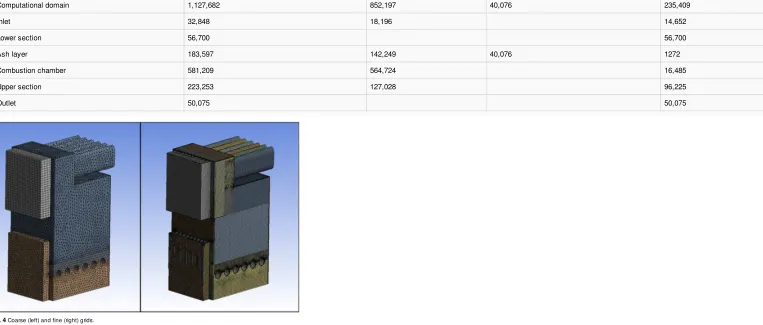
In order to perform the final simulations, a fine grid was used. It is a hybrid mesh, as it consists of a combination of element types, i.e. tetrahedrons, wedges, pyramids and hexahedrons. It contains close to 1.1 million cells, where their distribution in the computational domain as well as their composition are displayed in Table5. It is obvious that over of 50% of the mesh elements are located at the combustion chamber section, where the volumetric reactions are taking place. The mesh quality remains high with a maximum cells cell skewness of 0.936 and a minimum orthogonal quality of 0.14. Both coarse and fine meshes are presented in Fig.4.

Table5 Fine mesh element composition and distribution.

Computational domain 1,127,682 852,197 40,076 235,409

Inlet 32,848 18,196 14,652

Lower section 56,700 56,700

Ash layer 183,597 142,249 40,076 1272

Combustion chamber 581,209 564,724 16,485

Upper section 223,253 127,028 96,225

Outlet 50,075 50,075

A main feature of the fine mesh (Fig. 5), which is absent from the coarse one, is the imposition of twoinflation layers on all the walls that are in contact with water.In this way, a more accurate calculation of the heat flux deploying on the boiler walls is possible. The total boundary layer thickness is 6mm.

2.1.4 Boundary conditions

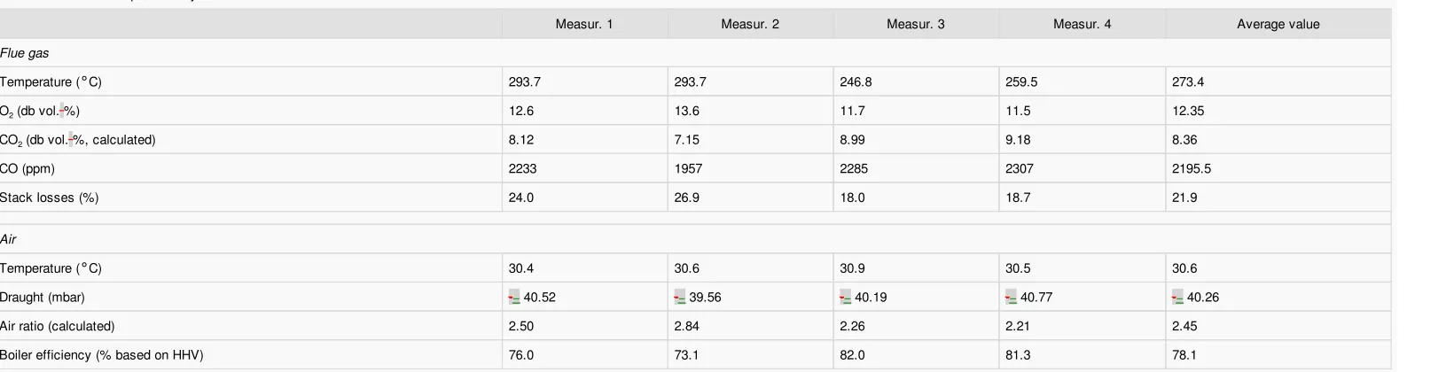
As was stated above, the examined boiler has only one air inlet. There is no secondary air stream. The determination of the air mass flow rate is based on the fuel chemical analysis as well as on four experimental measurements provided by the manufacturer. The latter were performed with a Bacharach PCA-3 and are presented on in Table6. The measurement point locates at the end of a 20cm long tube connected to the boiler’'s chimney exit.

Table6 Measurements provided by the boiler manufacturer.

Measur. 1 Measur. 2 Measur. 3 Measur. 4 Average value

Flue gas

Temperature (

°

O2 (db vol.%) 12.6 13.6 11.7 11.5 12.35

CO2 (db vol.%, calculated) 8.12 7.15 8.99 9.18 8.36

CO (ppm) 2233 1957 2285 2307 2195.5

Stack losses (%) 24.0 26.9 18.0 18.7 21.9

Air

Temperature (

°

Draught (mbar) -− 40.52 -− 39.56 -− 40.19 -− 40.77 -− 40.26

Air ratio (calculated) 2.50 2.84 2.26 2.21 2.45

Boiler efficiency (% based on HHV) 76.0 73.1 82.0 81.3 78.1

Based on the average value of the O2 concentration, the air to fuel ratio λ is computed using the following equation[21]:

, which results in an air ratio equal to 2.444. The combustion stoichiometric dry air mLoT′, is approximated using the raw fuel ultimate analysis by the following equation:

Thus the required stoichiometric dry air is 5.65kg/kg fuel. The dry air during the boiler tests can be computed by Eq.(22).

This gives 13.81kg dry air/kg fuel. The maximum water concentration in air which corresponds to the ambient air temperature is 0.027125kg/kg wet air. According to meteorological data, the relative humidity in July (the month in which the measurements were performed) at the region of Ptolemaida was 40%, resulting in a water concentration of 0.01085kg/kg wet air. The total wet combustion air is 13.96kg/kg fuel, calculated by Eq.(23).

The raw fuel mass flow is 0.001853kg/s, as computed by the reported nominal boiler power of around 32kW and the fuel LHV, using the following equation.

Thus the total air flow rate can be specified as 0.026kg/s, with an inlet temperature of 30.6 °C.

As far as the wall boundaries of the boiler are concerned, they can be summarized in 3 groups:

•The walls in contact with water. It was reported by the manufacturer, that during the experimental measurements the inlet water temperature was 60 °C and the outlet one equal to 70 °C, resulting in a mean water temperature of 65 °C. This temperature condition is applied to all the walls of

this group.

•The insulated walls that are not in contact with the operating medium. In this case a zero heat flux boundary condition is set as a boundary condition.

•The base of the boiler. In this case a constant temperature equal equals to the ambient one, i.e. 30.6 °C is applied, since this side of the boiler is not reported to be insulated and in direct contact with the earth surface.

In all the above cases, the wall emissivity is set to 0.9 and the radiation boundary condition to be opaque.

Since the inner part of the wood logs is considered to be solid body, these surfaces represent another group, where a “wall” type boundary conditions are applied. In order to steer the volatiles release released from the wood logs log base, the following temperature boundary conditions are set:

•A constant temperature of 900 °C is applied to the sides and the top of the logs, which is equal to typical the typically measured ones.

•A higher temperature of 1000 °C is applied to the base of the logs.

The selection of these temperatures is based on the fact that the decomposition of lignin takes place in a wide range of temperatures as high as 900 °C. Their internal emissivity is set to 0, otherwise the log walls irradiate unwanted heat inside the boiler.

As far as the fuel input power is concerned, it was revealed that in order to achieve the reported 22kW thermal output the required fuel power should be around to 32kW. The value of 22kW was used as a reference point, since this is the useful heat output that the manufacturer measures experimentally by monitoring water inlet and outlet temperature. From the quantity of 32kW, 12.01kW are is produced by the fixed char burnout and are is simulated as a heat source placed within the firebed-zone. The rest of heat release, i.e. 19.99kW, is imported in the computational domain owed to the combustion of the produced volatiles. However, the volatiles volatile combustion is not complete and a very small proportion reaches the boiler outlet unburnt. Furthermore, the CO burnout into CO2 is not complete too. Thus, the heat of the reactions which take takes place inside the boiler is smaller than the sum of the imported volatiles' heating value. Specifically, the heat due to reactions is 19.04kW resulting in an actual total thermal input

of 31.05kW.

2.1.5 Applicability of the model

Log wood boilers typically are not designed for load modulation. Therefore, the reference condition – and the ones which is of major importance for the EN303-5 type tests – is the full load. In principle, the model developed in this study can be used for partial loads or during transitory phases of operation, e.g. the start-up phase. For this case, it would need to take into account additional reactions, such as the Boudouard and water-–gas shift. Additionally, for the simulation of transitory phases, the boiler

(20)

(21)

(22)

undergoes, during its start-up or cooling down, the model would require a non-steady formulation and solution, which is computationally very expensive keeping in mind that the solution time-step would be within a range of ms so that the Courant number is less than 0.5. For these reasons, it was decided to focus the present work on the steady state modeling of the full load conditions.

3 Results and discussion

3.1

Simulation results of current boiler design

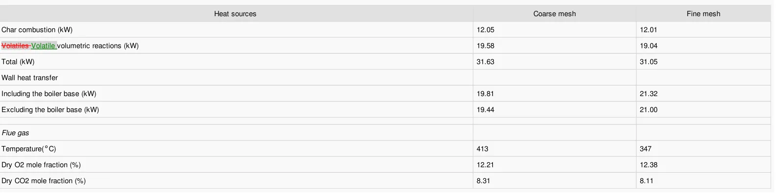
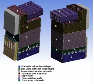
Simulation results of current boiler design Table 7 shows the simulation results concerning the heat transfer distribution inside the boiler, as well as the heat sources. The correspondence of each wall section to the boiler geometry is displayed in Fig. 6. The resulted resulting heat transfer of 21.32 kW (or 21 kW if the base walls are excluded) is in quite good agreement with the values reported by the manufacturer. It should also be noted that the net heat transfer of the log walls is negligible (they represent a source of 19 wattsW), thus the applied temperature boundary condition does not affect the heat transfer simulation.

Table7 CFD heat transfer results.

Heat sources Coarse mesh Fine mesh

Char combustion (kW) 12.05 12.01

Volatiles Volatile volumetric reactions (kW) 19.58 19.04

Total (kW) 31.63 31.05

Wall heat transfer

Including the boiler base (kW) 19.81 21.32

Excluding the boiler base (kW) 19.44 21.00

Flue gas

Temperature(

°

Dry O2 mole fraction (%) 12.21 12.38

The applied numerical grid contains close to 1.1 million cells. This mesh resolution can safely be considered as adequate for the discretization of a domestic 32 kW boiler. In similar CFD studies of large scale boilers coarser numerical grids have been implemented with success. [12] used a mesh of around 217,000 cells for investigating a 320 kW wood chip fired residential boiler, whereas [15] performed a design optimization study of a 180 kW biomass furnace using computational grids consisting of 700,000 cells. Nevertheless, a coarse grid of 240,000 elements was also used to check to what extent a relevant coarse grid can be regarded as enough for valid numerical results. The main results of this analysis are summarized in the table below and compared against the final numerical results.

The differences in flue gas O2 and CO2 mole fraction are small, i.e. 1.4% and 2.5% respectively. The difference of the induced wall heat flux is 7%, whereas flue gas exit temperature presents a considerable deviation between the numerical results in the

order of 19%. This high difference can be attributed to the lack of dense grid at the proximity of the surfaces adjacent to the cooling medium (water), and therefore the underestimation of wall heat flux. For that reason inflation layers were implemented. In conclusion, the fine grid employed in this work can reasonably be considered as adequate for providing accurate numerical results.

Table 8 summarizes the CFD results concerning the flue gas properties and the corresponding average experimental data. The reported values represent a mass-weighted calculation at the exit of the 6 flue gas tubes. As can be observed, the predicted

flue gas composition is in very good agreement with the measurements. The differences in O2 and CO2 mole fraction are 0.2% and 3% respectively. The stronger numerical and experimental disagreement concerning CO2 can be attributed to the fact that its

concentration is not measured directly by the measurement equipment, but is calculated on the basis of measured O2 concentration. This computation does not take into consideration the exact fuel chemical analysis, because it is based on a fixed biomass

composition available in the instrument database.

Table8 Comparison between CFD and experimental results.

Flue gas parameter CFD results Average experimental data

Temperature (

°

Dry O2 mole fraction (%) 12.38 12.35

Dry CO2 mole fraction (%) 8.11 8.36

Dry CO (ppm) 755 2195.5

Additionally, the CO deviation of the numerical prediction from the average measured one is quite high for reasons linked with the set of homogeneous and heterogeneous reactions considered in this study (for example we neglect the reaction of char and/or CO with H2O, while char is reacting with O2 to form only CO2 and not CO).

The CFD predicted flue gas temperature at the boiler exit is rather high, compared to the measured one. Even the highest measured temperature is 53 °C lower than the computed one. A valid explanation of this disagreement is the fact that the measurement point is not located at the elliptical tubes’' exit, but at about 35 cm downstream.

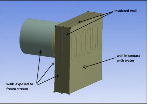
In order to verify this assumption an additional numerical calculation is conducted just at the outflow conjoiner part and the additional 20 cm long cylindrical tube (Fig. 7). As inlet quantities the corresponding ones at the exit of the 6 elliptical tubes are used. Three types of thermal boundary conditions are applied:

•To the base of the conjoiner part which is contact with water, a fixed temperature condition of 65 °C (equal to the water temperature).

•A zero heat flux condition to the section of the conjoiner wall which is covered by the fiberglass insulation layer.

•A convection thermal condition to all the other walls. The free stream temperature is set equal to that of the inlet air (30.6 °C), while a heat transfer coefficient of 10W/m2_{K is considered.}

The resulted resulting temperature at the end of the 20 cm long tube is 312.6 °C, reduced by 34.4 °C. Therefore, its difference from the highest computed temperature is 18.9 °C, a quite acceptable value. Another noteworthy conclusion is the fact that the heat transfer to the conjoiner base is 0.613 kW. Thus, the total heat transfer to the boiler walls is 21.93 kW or 21.62 kW excluding the heat flux to the boiler base, quite close to the reported values by the manufacturer. An equal heat of 0.61 kW is conveyed to the free stream.

As far as the spatial distribution of the simulation variables is concerned, two representative planes corresponding to each wood log position are selected. These are displayed in Fig. 8.

Fig. 9 depicts the temperature spatial distribution in the two reference planes. The maximum temperature in the boiler is 1507 °C. According to literature, temperatures over 1000 °C are to be expected in boilers of similar technical characteristics [22], whereas temperatures as high as 1500 °C have been reported in equivalent CFD studies [17]. Noteworthy is the fact that in both planes high temperatures are located close to the log bases. This pattern corresponds to the char combustion volumetric heat source (Fig. 10) and can be attributed to it.

Fig. 8 Boiler reference planes: y= -− 0.2m (left) & y = -− 0.33m (right).

As can be observed in Fig. 11 the wood volatiles are released from the desirable area, i.e. from the log bases. The O2 molar concentration reduction (Fig. 12) corresponds to the areas where reactions take place and as expected its distribution pattern is

opposite of that of CO2 (Fig. 13). In the same figures an O2 sink and a corresponding CO2 increase can be spotted at the ash layer and are also related to the char combustion volumetric mass sources. Another conclusion extracted from these figures is the fact that

in the two reference planes, the distribution of the above referred variables is different. Several CFD tests revealed that the log geometry affects the volatiles combustion pattern in a great extent. Thus these differences can be attributed to the different cross-section area areas of the two logs (Fig. 8).

Fig. 10 Spatial distribution of the char combustion volumetric heat source (W/m3_).

The Reynolds number calculated using as a reference length the average cell edge for all computational cells is depicted in Fig. 14. The range of values is between 0.43 and 110, with the maximum values located at the proximity of the porous media area, where the flue gas velocity accelerates (~ 110) and within the flue gas tubes (~ 72). For the boiler volume above the porous, flue gas experience Reynolds of the order 60, while below the Re number equals to around 15. As a general conclusion, the flue gas flow is mainly dominated by inertia when compared to viscous forces, with the exception of a) the boiler volume located just below the porous media, b) the volume located at the level of the transition zone side walls (D in Fig. 6) and c) the boiler upper wall (E

in Fig. 6), before the flue gas enters the tubes.

Fig. 12 Spatial distribution of the dry O2 mole fraction at the two reference planes.

The flue gas flow in the form of dimensionless numbers can be characterized by the above-mentioned Re contour, while the heat transfer mechanisms towards the boiler water filled walls by the corresponding Nu contour. Nu is calculated only at the proximity of wall surfaces and using as a reference length the value of 1 m. The maximum values are calculated in the range of ~ 21,500 located at the entrance of the flue gas tubes, Fig. 15. An average Nu number of around 7510 is calculated at the proximity of water surfaces, while the minimum heat flux takes place just below the porous media zone.

As far as the chemical phenomena are concerned, it is not a standard practice to use dimensionless variables for their characterization. The chemical reaction rates are calculated using Arrhenious-type equations. Mostly, what can be said is that homogeneous reactions are turbulence instead of kinetic driven; the overall rate rates of reactions (1) and (2) are 0.037and 0.06 k mol/m3_{s respectively.}

3.2 Simulation results of an optimized boiler design

Fig. 14 Spatial distribution of the Reynolds number.

3.2.1 Modification description

The second phase of the project includes the numerical simulation of an optimized boiler design. The main objectives of this research are:

•the increase of the boiler efficiency and

•the emission reduction. Since the developed numerical model does not include NOx calculations, the main pollutant specie under consideration is CO.

A common way to achieve both of these goals is to increase the flue gas residence time. The longer the flue gases remain inside the boiler, the more its combustion is expected to be complete. In that way, an almost zero pollutant emission and a maximum heat of reaction release can be achieved.

However, the proposed design modifications could not be extensive and have to be in accordance with the existing boiler layout and operational restrictions (wood loading). The corresponding financial cost and constructional difficulties imposed by the boiler geometry, constrain further the available options. In this framework, the proposed arrangement involves the placing of a deflector upstream of the elliptical flue gas tubes (Fig.16).

This is a low-cost and easily actualized alteration, since a common steel sheet can be used as deflector. The latter is expected to impose a barrier on the flue gas flow towards the boiler chimney, increasing its residence time at the combustion chamber. However, the corresponding static pressure drop should be kept at reasonable limits, otherwise the deflector in combination with the lack of a ventilator could disturb the boiler operation. For this reason, a high part of the available boiler free cross-section cannot be covered by the metal sheet (Fig.17).

The proposed optimized solution was selected as the optimum one among many concepts examined (e.g. use of secondary air, imposition of more water tubes). The reasons are that a) it has a very low cost of manufacturing (around 400€/boiler) and b) the available free space within the boiler for further design improvements is very limited (imposed by the water and flue-tubes), for loading purposes. The solution has not yet been tested in field since in the current period the boiler production line cannot be interrupted; however, the manufacturer aims to construct and test the new boiler design within the next 6months.

3.2.2 Comparison of original and optimized design

In order to simulate the new proposed boiler setup, a new mesh is developed. Similar to the basic scenario, the hybrid mesh consists of 1.3 million cells, with almost half of them to discretize the main combustion chamber of the boiler.

As far as the numerical set-up is concerned, the same numerical models with the basic geometry simulation are used. In order to compare the two designs under the same operational conditions, the boundary conditions are not altered too. The total air flow rate is specified equal to 0.026kg/s, with an inlet temperature of 30.6 °C. The fuel input power is 32kW, 12.01kW of which are attributed to the fixed char burnout and simulated as volumetric heat source placed within the firebed-zone. The rest 19.99kW

represent represents the heat released from the volatiles volatile combustion. Due to their incomplete burnout, the heat due to reactions is 19.14kW resulting in a total thermal input of 31.15kW, very close to the 31.05kW of the basic case.

I n Table9 the comparison of the two design simulation results concerning the heat transfer distribution inside the boiler is displayed. The correspondence of each wall section to the boiler geometry is displayed in Fig.6. It is obvious that the

resulted resulting heat transfer for the optimized design is considerably improved. A total heat of 23.50kW (or 23.16kW if the base walls are excluded) is absorbed by the boiler walls, resulting in an efficiency increase of 6.7%. As far as the heat distribution is concerned, the main differences are spotted at the upper part of the boiler, i.e. at the combustion chamber, the front water tube, the transition zone, and the upper walls. A heat transfer increase between 22.3% and 55.2% is reported in these zones, resulting in a gain of 3.72kW. On the other hand, the heat absorbed by the elliptical tube walls is reduced by 1.66kW, Table9. This can be attributed to the effect of the deflector on the induced flue gas flow characteristics. The non-uniform reduction of the available free cross-section, results in an increase of the flue gas velocity towards the boiler outlet and thus a subsequent decrease of the flue gas residence time for this area. Nevertheless, the overall effect of the deflector is proven to be positive.

Table9 Comparison of the CFD heat transfer results between the two boiler designs.

Heat sources Original design Optimized design

Due to char combustion (kW) 12.01 12.01

Due to volatiles

’

Total (kW) 31.05 31.15

Wall heat transfer

Base walls (kW) 0.316 0.344

Side walls below the ash layer 0.075 0.106

Side walls at the ash layer height 0.579 0.653

Water tubes (kW) 1.621 1.776

Front rectangular water tube (kW) 0.907 1.408

Combustion chamber side walls (kW) 3.846 4.495

Transition zone side walls (kW) 2.981 4.495

Upper walls (combustion chamber & transition zone) (kW) 3.342 4.230

Elliptical tubes

’

Total (kW) 21.322 23.501

Table10 shows the flue gas properties in both cases. In accordance with the heat transfer results, the flue gas temperature is decreased by 18.4% in the case of the optimized scenario. The differences in O2 and CO2 mole fraction are very small, i.e. 0.6%

and 0.37% respectively. As far as the CO concentration is concerned, again as in the reference scenario the resulted value is significantly smaller than the corresponding measurement value (Table6) and that of the reference one. As a matter of fact, a reduction of almost 45% is achieved in the optimized design. Although this decrease concerns only the volatiles volatile combustion, it is an important improvement.

Table10 Comparison of the flue gas properties.

Flue gas parameter Original design Optimized design

Temperature (

°

Dry O2 mole fraction (%) 12.38 12.46

Dry CO2 mole fraction (%) 8.11 8.08

Dry CO concentration (ppm) 755 417

All aforementioned improvements are linked with the higher residence time of the flue gas, thus giving it more time to interact with the boiler water surfaces and transfer more energy, which in turn increases the boiler efficiency. Additionally the fact that the exit CO concentration decreases is linked to the fact that more time is available for it to react with O2 and form CO2. In our view, though the calculated CO values may differentiate from real data, the trend should be that of its decrease in the optimized boiler

geometry.

In the case of the modified geometry, the numerical calculation at the outflow conjoiner part and the additional 20cm long cylindrical tube (Fig.7) is also conducted. The resulted resulting temperature at the end of the latter is 256.8 °C, reduced by 26.2 °C and quite lower than that of the basic scenario (312.6 °C). The heat transfer to the conjoiner base is 0.430kW, while 0.473kW are is conveyed to the free stream.

The positive effect of the deflector on the temperature distribution upstream the flue gas tubes can be observed in Fig.19. The presented plane is located 0.041m before their entrance. Furthermore, in the optimized design there is a wider area of high temperature inside the boiler. The increased heat flux at the combustion chamber and the transition zone are is in agreement with this scheme.

Fig.20 depicts the volatiles volatile volumetric mass source in the optimized scenario. Their emission scheme is identical to that of the basic case, as they are likewise released from the wood logs log bases. The O2and CO2molar concentrations are

displayed in Figs.21 and 22, respectively. As was anticipated, their distribution patterns are inverse. Moreover, in this simulation too there are differences between the two reference planes. However, in agreement with the temperature dispensation, downstream of the deflector the variations are negligible.

Fig.18Contours of spatial temperature (K) distribution at the two reference planes: y = -− 0.2 (left) & y = -− 0.33 (right) – — optimized design.

Fig.20Spatial distribution of the volatiles volumetric mass source (kg/m3_{s) at the two reference planes: y = -− 0.2 (left) & y = -− 0.33 (right) – — optimized design.}

4 Conclusions

A simplified CFD model focused on the flue gas side has been developed and used for the steady-state simulation of a 32 kW boiler manufactured by the Greek company THERMODYNAMIKI S.A. (KOMBI). Its main characteristic is the fuel division into water vapor, volatiles and fixed char, and the assignment of each component to separate zones. Volatiles and vapor are released from the log's outer layer, while the fixed char burnout takes place in the firebed. The numerical results are in quite good agreement with experimental data concerning the flue gas characteristics at the boiler exit (temperature and species concentration) and the boiler thermal efficiency.

In order to improve flue gas burnout, to increase the boiler efficiency as well as to reduce CO emissions a simple and low-cost modification of the boiler design has been proposed and examined by means of CFD. It involves the placing of a deflector upstream of the flue gas tubes and aims in increasing the flue gas residence time at the combustion chamber. The numerical simulation of the modified design reveals a considerable improvement of the boiler characteristics.

Concluding, CFD models, such as the one presented in this report, can be employed for the realistic simulation of wood log fired boilers. Because of their flexibility, they can be used as a tool not only for efficiency analysis, but also

as for design optimization purposes. Nevertheless, their extensive validation against experimental data is necessary to optimize the model setup and thus increase further the accuracy of the numerical results. In the current case, the experimental measurements performed by the manufacturer were rather confined, resulting in limitations of the model validation. The implementation of new series of measurements either in the original boiler or in the modified design and their comparison with the CFD results, would definitely help to improve the setup of the proposed model and verify its usage further as an optimization tool.

This is quite important since simple modifications can improve the boiler characteristics in a considerable extent. The current model of boiler (original design) belongs to Class 3 of EN303-5 standard (Heating boilers - –Part 5: Heating boilers for solid fuels, manually and automatically stoked, nominal heat output of up to 500 kW -–Terminology, requirements, testing and marking) which is the threshold for the introduction of a domestic solid biofuel boiler to the Greek market. According to the manufacturer, for a nominal output of 30 kW, the boiler’'s efficiency is above 75.86% and CO concentration is below 5000 mg/m3 _{(class 3 limits satisfied). However, according to the CFD model, the optimized boiler is expected to have an}

increased efficiency by around 7% and reduced CO emissions by almost 45%. This means that the modified boiler will be very close to the satisfaction of Class 4 limits (efficiency above 82.95% and CO concentration below 1200 mg/m3_{) giving}

the chance to the manufacturer to upgrade its current model with a few non expensive modifications on the current design (lower than 400 €/boiler).

Acknowledgments

The boiler manufacturer, Thermodynamiki S.A. (KOMBI) provided useful data regarding the design and operation of the boiler along with experimental data (flue gas temperature, O2, CO, CO2 concentration etc.) for proper determination

of the boundary conditions imposed in the simulation.

The study described in this publication was financially supported by the Greek General Secretariat for Research and Technology (GSRT) within the frame of “ΠρόγραµµαΑνάπτυξηςτηςΒιοµηχανικήςΈρευναςκαιΤεχνολογίας

(ΠΑΒΕΤ)” call for projects. The enumerated code of the Project is 326-BET (ΠΥΡΚΑΛ).

References

[1]

Forestry in the EU and the World - — a Statistical Portrait, 2011, eurostat.

[2]

Production and Consumption of Wood in the EU27, 2012, (eurostat news release, 168/2012).

[3]

A. Strehler, Technologies of wood combustion, Ecol. Eng.16 (Supplement 1(0)), 2000, 25–40.

[4]

A. Anca-Couce, et al., Smouldering of pine wood: kinetics and reaction heats, Combust. Flame159 (4), 2012, 1708–1719.

[5]

S.Y. Yorulmaz and A.T. Atimtay, Investigation of combustion kinetics of treated and untreated waste wood samples with thermogravimetric analysis, Fuel Process. Technol.90 (7-8), 2009, 939–946.

[6]

M. Amutio, et al., Pyrolysis kinetics of forestry residues from the Portuguese Central Inland Region, Chem. Eng. Res. Des.91 (12), 2013, 2682–2690.

[7]

G. Skodras, et al., Pyrolysis and combustion characteristics of biomass and waste-derived feedstock, Ind. Eng. Chem. Res.45 (11), 2006, 3791–3799.

[8]

C. Di Blasi, Modeling chemical and physical processes of wood and biomass pyrolysis, Prog. Energy Combust. Sci.34 (1), 2008, 47–90.

[9]

C. Bruch, B. Peters and T. Nussbaumer, Modelling wood combustion under fixed bed conditions, Fuel82 (6), 2003, 729–738.

[10]

J. Collazo, et al., Numerical modeling of the combustion of densified wood under fixed-bed conditions, Fuel93 (0), 2012, 149–159.

[11]

M.A. Gomez, et al., CFD modelling of thermal conversion and packed bed compaction in biomass combustion, Fuel117 (Part A(0)), 2014, 716–732.

[12]

X. Zhang, et al., Experimental investigation and mathematical modelling of wood combustion in a moving grate boiler, Fuel Process. Technol.91 (11), 2010, 1491–1499.

[13]

J. Collazo, et al., Numerical simulation of a small-scale biomass boiler, Energy Convers. Manag.64, 2012, 87–96.

[14]

J. Chaney, H. Liu and J. Li, An overview of CFD modelling of small-scale fixed-bed biomass pellet boilers with preliminary results from a simplified approach, Energy Convers. Manag.63, 2012, 149–156.

[15]

Queries and Answers

Query:

Your article is registered as a regular item and is being processed for inclusion in a regular issue of the journal. If this is NOT correct and your article belongs to a Special Issue/Collection please contact [email protected] immediately prior to returning your corrections.

Answer: The paper is a regular article

Query:

Please confirm that given names and surnames have been identified correctly.

Answer: These are correct

Query:

R. Scharler, et al., CFD based design and optimisation of wood log fired stoves, In: 17th European Biomass Conference and Exhibition, From Reserch Research to Industry and Markets, 2009, (Hamburg, Germany).

[17]

R. Scharler, et al., CFD simulations as efficient tool for the development and optimisation of small-scale biomass furnaces and stoves, In: 19th European Biomass Conference & Exhibition, 2011, (Berlin, Germany).

[18]

R. Peyret, Handbook of Computational Fluid Mechanics, 1996, Academic Press Limited; USA.

[19]

C. Hirsch, Numerical Computation of Internal and External Flows, 1990, T. Francis, (Ed.).

[20]

S.V. Patankar, Numerical Heat Transfer and Fluid Flow, 1980, T. Francis, (Ed.).

[21]

PCA 3 Portable Combustion Analyzer - — Operation and Maintenance Manual, 2011.

[22]

Log wood boilers.

Highlights

•A numerical model for wood log combustion has been developed.

•Fuel in the developed model includes water vapor, volatiles and fixed char.

•Simulation model is validated through experimental measurements.

•New boiler modification results in the increase of boiler efficiency by around 6.7%.

Please check that the affiliations link the authors with their correct departments, institutions, and locations, and correct if necessary.

Answer: Affiliation details are correct

Query:

One parenthesis has been added to balance the delimiters. Please check that this was done correctly, and amend if necessary.

Answer: Correct comment

Query:

One parenthesis has been added to balance the delimiters. Please check that this was done correctly, and amend if necessary.

Answer: Correct comment

Query:

The term "referenced" has been changed to "references". Please check if this change is appropriate, and amend if necessary.

Answer: correct change

Query:

The given sentence seems to be incomplete. Please check for missing words/phrases and complete the sentence.

Answer: correct change

Query:

"ap" has been changed to "αp". Please check, and correct if necessary.

Answer: correct change

Query:

Please note that Table 3 was not cited in the text. Please check that the citation suggested by the copyeditor is in the appropriate place, and correct if necessary.

Answer: correct change

Query:

This sentence has been slightly modified for clarity. Please check that the meaning is still correct, and amend if necessary.

Answer: we approve

Query:

The decimal point has been changed to a decimal comma in 240,000. Please check, and correct if necessary.

Answer: I approve

Please note that Fig. 5 was not cited in the text. Please check that the citation suggested by the copyeditor is in the appropriate place, and correct if necessary.

Answer: Correct addition

Query:

"Simulation results of current boiler design" was captured as subsectionn 3.1 and following subsections were renumbered. Please check and correct if necessary.

Answer: Correct

Query:

Please supply the name of the publisher.

Answer: R. Scharler, C. Benesch, A. Neudeck, I. Obernberger. CFD based design and optimisation of wood log fired stoves. G.F. De Santi (Ed.), 17th European biomass conference & exhibition; June 2009; Hamburg;

Germany, ETA-Renewable Energies, Florence; Italy (2009), pp. 1361–1367

Query:

Please supply the name of the publisher.

Answer: R. Scharler, C. Benesch, K. Schulze, I. Obernberger. CFD simulations as efficient tool for the development and optimisation of small-scale biomass furnace and stoves. M. Faulstich (Ed.), 19th European biomass

conference & exhibition; June 2011; Berlin; Germany, ETA-Renewable Energies, Florence; Italy (2011), pp. 4–12

Query:

Please provide the complete details for Reference [22].

Answer: Publisher: Paul Künzel GmbH & Co., Paul Künzel GmbH & Co. · Ohlrattweg 5 · D-25497 Prisdorf The name of brochure is "Log wood boiler" if more info is required please visit the following link: