A Maximal Clique Based Multiobjective
Evolutionary Algorithm for Overlapping
Community Detection
Xuyun Wen, Student Member, IEEE, Wei-Neng Chen, Member, IEEE, Ying Lin, Member, IEEE, Tianlong Gu,
Huaxiang Zhang, Yun Li, Member, IEEE, Yilong Yin, and Jun Zhang, Senior Member, IEEE
Abstract—Detecting community structure has become one
important technique for studying complex networks. Although many community detection algorithms have been proposed, most of them focus on separated communities, where each node can belong to only one community. However, in many real-world networks, communities are often overlapped with each other. Developing overlapping community detection algorithms thus becomes necessary. Along this avenue, this paper pro-poses a maximal clique based multiobjective evolutionary algorithm (MOEA) for overlapping community detection. In this algorithm, a new representation scheme based on the intro-duced clique graph is presented. Since the maximal-clique graph is defined by using a set of maximal maximal-cliques of original graph as nodes and two maximal cliques are allowed to share the same nodes of the original graph, over-lap is an intrinsic property of the maximal-clique graph. Attributing to this property, the new representation scheme allows MOEAs to handle the overlapping community detection problem in a way similar to that of the separated com-munity detection, such that the optimization problems are simplified. As a result, the proposed algorithm could detect overlapping community structure with higher partition accuracy and lower computational cost when compared with the existing ones. The experiments on both synthetic and real-world net-works validate the effectiveness and efficiency of the proposed algorithm.
Manuscript received February 24, 2016; revised June 30, 2016; accepted August 19, 2016. Date of publication September 1, 2016; date of current version May 25, 2017. This work was supported by the National Natural Science Foundation of China under Grant 61622206, Grant 61332002, Grant U1201258, and Grant 61309003. (Corresponding
authors: Wei-Neng Chen; Jun Zhang.)
X. Wen is with the School of Computer Science and Engineering, South China University of Technology, Guangzhou 510006, China, and also with the Sun Yat-sen University, Guangzhou 510006, China.
W.-N. Chen and J. Zhang are with the School of Computer Science and Engineering, South China University of Technology, Guangzhou 510006, China (e-mail:[email protected];[email protected]).
Y. Lin is with the Department of Psychology, Sun Yat-sen University, Guangzhou 510006, China.
T. Gu is with the School of Computer Science and Engineering, Guilin University of Electronic Technology, Guilin 541004, China.
H. Zhang is with the School of Information Science and Engineering, Shandong Normal University, Jinan 250014, China.
Y. Li is with the School of Computer Science and Network Security, Dongguan University of Technology, Dongguan 523808, China.
Y. Yin is with Shandong University, Jinan 250100, China.
This paper has supplementary downloadable multimedia material available athttp://ieeexplore.ieee.orgprovided by the authors.
Color versions of one or more of the figures in this paper are available online athttp://ieeexplore.ieee.org.
Digital Object Identifier 10.1109/TEVC.2016.2605501
Index Terms—Clique-based representation, maximal-clique
graph, multiobjective evolutionary algorithm (MOEA), overlapping community detection.
I. INTRODUCTION
R
ECENT years have witnessed many researches that modeled real-world systems in nature and society as networks to capture the intricate properties of these complex systems, where objects are represented as nodes and the interactions among the objects are represented as edges [1]–[5]. Uncovering the community structure of com-plex networks is helpful for understanding comcom-plex sys-tems. Researches on analyzing community structure thus gained growing attention during the past decades [6]–[9]. Traditionally, much of the focus within community detec-tion is on the separated communities, where each node can belong to only one community [6], [7], [10], [11]. However, in many real-world networks, communities are often over-lapped with each other [12]–[15]. For example, people in social networks always belong to several groups, simulta-neously, such as family, friends and colleagues. For this reason, recent studies have paid much attention to overlapping community detection and developed various algorithms from different perspectives, including clique percolation [12], link partitioning [13], local expansion and optimization [16], [17], and label propagation [18].The community detection problem can be formulated as an optimization problem [7], and such a problem is always NP-hard [19]. Therefore, some researchers introduced evolu-tionary algorithms (EAs) into this field and developed several promising methods [9], [20], [21]. In addition, it is widely accepted that a community should have dense intraconnections and sparse interconnections, implying that two conflicting objectives should be optimized simultaneously in commu-nity detection, i.e., maximizing internal links and minimiz-ing external links [6], [22], [23]. Therefore, the community detection problem can also be modeled as a multiobjec-tive optimization problem (MOP). Along this line, several multiobjective EAs (MOEAs) [19], [24]–[28] have been pro-posed. However, most of them focused on separated com-munity detection and failed to detect overlapping comcom-munity structures.
In fact, one obstacle for applying MOEAs to overlapping community detection is the representation scheme of the individual. The existing representation approaches can be broadly divided into two major classes, i.e., prototype-based approaches [28] and node-based approaches [24]–[27]. In the prototype-based approaches [28], each gene of an individual represents the information of one community, e.g., the coordinates of the community center. Though suitable for overlapping community detection, this representation scheme has some shortcomings and limitations, such as tending to capture round-shaped community, requiring to set the num-ber of communities in advance, and increasing the difficulty in designing evolutionary operators. Furthermore, when adopt-ing prototype-based approaches as the representation scheme, the community detection is generally converted to a data clus-tering problem, which is based on the network information such as spectrum [28]. During this transformation, some valid network information may be lost [28].
Unlike the prototype-based representation, genes of an individual in the node-based approaches correspond to the community information of the nodes in the network [24]–[27]. Under this scheme, there are two types of approaches: 1) direct and 2) indirect. For the direct node-based approach [24]–[27], each gene is an integer representing the community infor-mation of the corresponding node, such as the label of the community this node belongs to [27] or the label of a node that belongs to the same community with this node [24]–[26]. However, since this representation scheme can only ensure every node to be assigned to one community, it is not suitable for overlapping community detection. For the indirect node-based approach [27], each gene of an individual is a random integer within the number of nodes of the network and thus a decoder is needed to transform them to the corresponding community information. In the decoding process, each node is allowed to belong to multiple communities, such that this representation approach can be used for overlapping commu-nity detection. However, the introduction of the decoder in the evolution process brings in two main drawbacks. First, since the fitness computation is directly related to the decoder, the decoding method has a significant influence on partition accuracy. Second, the decoding process is executed for each individual in each generation, leading to a high computational complexity of the algorithm.
To address the aforementioned issues of representation schemes, this paper introduces the maximal-clique graph, which uses a set of maximal cliques as nodes and links among maximal cliques as edges. Then based on the maximal-clique graph, a clique-based representation scheme is proposed, where each gene of the individual represents the commu-nity label of the corresponding maximal clique. Since two maximal cliques are allowed to share the same nodes of the original graph, overlap is an intrinsic property of the nodes of the maximal-clique graph, which exactly character-izes the overlapping communities. Attributing to this property, the new representation scheme allows MOEAs to handle the overlapping community detection problem in a way similar to that of the separated community detection, which not only simplifies the optimization problems, but also overcomes some
limitations of the existing representation schemes. Compared with the prototype-based representation, the clique-based approach is not restricted by community shapes and requires no prior knowledge on the community structure. Compared with the indirect node-based representation, the clique-based approach does not need to decode individuals in the evolution process, which largely lowers the computational cost of the algorithm.
Afterwards, the clique-based representation scheme and the corresponding evolutionary operators are coupled with the framework of MOEA, constituting a maximal clique based MOEA (MCMOEA), for overlapping community detection. The experiments on synthetic networks and real-world net-works validate that MCMOEA is effective and efficient. Comparisons with other five representative algorithms show that MCMOEA is competitive and promising.
The rest of this paper is organized as follows. Section II briefly describes the community detection problem, and introduces the objective functions and the framework of MOEA used in this paper. Section III gives a detailed descrip-tion of the proposed maximal-clique graph. In Secdescrip-tion IV, the details of MCMOEA are presented. In Section V, the per-formance of MCMOEA is evaluated on both synthetic and real-world networks and the comparisons are made between MCMOEA and other five representative methods. Finally, the conclusion is given in Section VI.
II. BACKGROUND
This section introduces the necessary background knowledge for understanding the proposed MCMOEA. First, the definition of network community used in this paper is clarified. Then the multiobjective model of the community detection problem is given. In the end, the framework of MOEA used in this paper is briefly reviewed.
A. Definition of Network Community
A network can be modeled as a graph G = (V,E), where V = {v1,v2, . . . ,vN} is the set of nodes,
E = {(vi,vj)|vi,vj ∈ V and i=j} is the set of links, called
edges, and N is the number of nodes. Generally, a community in a network is regarded as a group that has dense intra-links and sparse inter-links. To make the definition more clear, Radicchi et al. [10] gave a quantitative description of the net-work community based on the node degree. Let A=[Aij]N×N
be the adjacent matrix of G. For an unweighted graph, Aij =1,
if (vi,vj) ∈ E; otherwise, Aij =0. Suppose S is a subgraph
of G, and then for any node vi ∈S, the internal and external
degrees of node vican be denoted as kinS(vi)=
vi,vj∈SAijand
koutS (vi)=
vi∈S,vj∈/SAij, respectively. Then S is a community
in a strong sense if
∀vi∈S,kinS(vi) >kSout(vi). (1)
In other words, every node in a strong community has more intraconnections than interconnections. In contrast, S is a community in a weak sense if
vi∈S
kinS(vi) >
vi∈S
That is, the sum of internal degrees of nodes in a weak com-munity is larger than that of external degrees. Considering the former community definition is too strict, the latter one is adopted in this paper [27].
B. Community Detection Problem
The community detection problem can be modeled as an MOP with two objectives [19], [24]–[28]. One objective is to maximize the link density among nodes in the same commu-nity (intra-link density), while the other is to minimize the link density among nodes in different communities (inter-link den-sity). A number of different criteria have been proposed for measuring intra-link and inter-link densities [19], [25], [26]. In this paper, the kernel k-means (KKM) [29] and ratio cut (RC) [26] are, respectively, adopted for measuring these two densities. Given a graph G and a partition C with t com-munities, let Vp ⊆ V be the set of nodes in a community
p(p = 1,2, . . . ,t) and Vp = V −Vp be the set of nodes
that are not in p. The KKM and the RC values of C can be calculated as
KKM=2(N−t)−
t
p=1
LVp,Vp
Vp (3)
RC=
t
p=1
LVp,Vp
Vp
(4)
where L(Vp,Vp) =
vi,vj∈VpAij and L(Vp,Vp) =
vi∈Vp,vj∈VpAij are the sum of internal and external link
strengths of nodes in Vp, respectively, and “| · |” denotes the
size of a set. Through (3) and (4), we can see that a small KKM value indicates that the communities in C have high intra-link densities, while a small RC value indicates that the commu-nities in C have low inter-link densities. Therefore, through using (3) and (4) as the objectives, the community detection problem can be formulized as an MOP that seeks minimization on both objectives.
C. MOEA/D
The main focus of this paper is to propose a new representation scheme for MOEAs to solve the overlapping community problems and address the limitations of the existing approaches. Therefore, based on the proposed rep-resentation scheme, different MOEAs could be adopted to implement MCMOEA, such as MOEA based on decom-position (MOEA/D) [30], non-dominated sorting genetic algorithm II (NSGA-II) [31], strength Pareto EA II [32], and MOEA with double-level archives (MOEA_DLA) [33]. However, to facilitate illustration, one of the most widely used MOEAs with relatively low computational complexity, i.e., MOEA/D [19], [26], [27], is chosen as the representa-tive in the following section for illustrating the structure of MCMOEA. The implementation details of MCMOEA with the frameworks of other MOEAs are provided in Section V-D. Therefore, in this section, only the procedure of MOEA/D is reviewed.
[image:3.612.373.504.54.156.2]As a decomposition-based method, MOEA/D [30] decom-poses an MOP into several scalar optimization subproblems
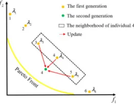
Fig. 1. Simple illustration of MOEA/D.
and optimizes them simultaneously. Each individual in the population of MOEA/D is associated with a subproblem and assigned an n-dimensional weight vectorλ=(λ1, λ2, . . . , λn),
where n is the number of objective functions. Based on the distance between the weight vectors, the neighborhood rela-tionships among subproblems are determined. Considering the fact that neighboring subproblems should have similar optimal solutions, each individual is optimized using only the information of its neighbors.
Fig. 1 exemplifies the idea of MOEA/D using an MOP with two objectives. In Fig. 1, the yellow curve represents the Pareto front (PF). Dots in different colors represent indi-viduals in different generations and red arrows indicate the evolutionary direction. The population evolution in MOEA/D consists of three steps. First, six individuals, each of which is associated with a subproblem, are initialized and assigned different weight vectors λ1,λ2, . . . ,λ6. Second, the neigh-borhood of each subproblem is determined according to the distance between the weight vectors. For example, suppos-ing that the neighborhood size is 3, individuals 3 and 5 are selected as the neighbors of individual 4. Third, each individual is optimized based on the information of its neigh-bors, e.g., individual 4 is updated based on individuals 3–5. For more detailed descriptions of MOEA/D, please refer to [30].
III. MAXIMAL-CLIQUEGRAPH
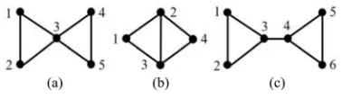
In this section, the definition and the construction method of the maximal-clique graph are introduced. As the basic unit of the maximal-clique graph, the concept of the maximal clique is given at first. Given a graph, a clique is a complete subgraph in which every two nodes are adjacent [34]. k-clique means the size of the clique is k. A maximal clique is a special clique which cannot be extended by adding any other nodes [34]. Take Fig. 2 as an example. Nodes v5,v6, and v7 compose a 3-clique, but it is not a maximal clique as it can be extended to a 4-clique by adding node v8.
Fig. 2. Examples of maximal cliques. Nodes v1, v2, and v3 constitute
maximal clique ①; nodes v3, v4, and v5 constitute maximal clique ②;
nodes v3, v5, and v6 constitute maximal clique③; nodes v5, v6, v7, and v8
constitute maximal clique④.
revelation of the overlapping structure. In order to detect communities from the perspective of maximal cliques, this paper proposes to convert the original graph G = (V,E) into a maximal-clique graph Gc = (Vc,Ec), where Vc = {vc1,vc2, . . . ,vcM} is named as clique nodes and Ec =
{(vcm,vcn)|vmc,vcn ∈ Vc and m = n}is named as clique edges or clique links, respectively. The conversion method contains three steps: 1) determining the clique nodes; 2) measuring the link strength between clique nodes; and 3) determining the clique edges based on the distribution of link strength. Detailed implementation of these three steps is described in the following parts and the corresponding flowchart is presented in Fig. S1 in the supplementary material.
A. Determining Clique Nodes of Maximal-Clique Graph Determining clique nodes is the first step to build a maximal-clique graph. In this paper, a set of maximal cliques in the original graph G are adopted as clique nodes of the corresponding maximal-clique graph Gc. Since each maximal clique is one of the largest cliques the nodes in G belong to, this paper transforms the determination process of clique nodes into finding all the largest clique(s) that each node in G belongs to, and designs the corresponding method as shown in Algorithm 1.
In Algorithm1, the clique nodes are determined in descend-ing order accorddescend-ing to their clique sizes. Since the nodes with higher degrees are more likely to constitute larger maximal cliques, the determination process first calculates the degree of each node in G and sorts the nodes in descending order of their degrees (lines 2–4). Suppose that the number of nodes of G is N and the largest node degree is kmax, then the size of cliques in G is not larger than (kmax+1). With k descending from (kmax+1) to 1, the determination process searches for the k-clique(s) of each node. As every two nodes in a clique are adjacent, the degrees of all nodes in a k-clique must be larger than (k−1). Additionally, since only the largest clique(s) for each node are interested, the searching process stops seek-ing smaller cliques for a node if it has been assigned to the larger ones. Therefore, the determination process only searches for k-clique(s) of a node when the following three conditions are satisfied: 1) the node degree is not smaller than (k−1) (lines 7–9); 2) the node has not been assigned to any cliques (lines 10–12); and 3) at least (k−1) adjacent nodes have a degree no smaller than (k−1) (lines 13–16). If all these conditions are satisfied, the determination process transforms the problem of finding all the k-clique(s) that contain this node to that of searching for the (k−1)-clique(s) constituted by
Algorithm 1 Determining the Clique Nodes of Gc
Input: Original graph G=(V,E); Output: Set of clique nodes Vc;
1: Vc←φ;
2: Calculate the degree k(vi)of each node vi∈V; 3: kmax←maxvi∈Vk(vi);
4: Sort the nodes in descending order of the degree; 5: for k=kmax+1 to 1 do
6: for each node vi∈V do
7: if k(vi) <k−1
8: no more k-cliques exist and goto Outer loop (Line 22);
9: end if
10: if vihas been assigned to one clique node
11: goto Inner loop (Line 20);
12: end if
13: Neigh(vi)← {vj|(vjis adjacent to viand kvj≥k−1}; 14: if|Neigh(vi)|<k−1
15: vicannot constitute k-cliques and goto Inner loop (Line 20);
16: end if
17: if the nodes in Neigh(vi) can constitute q (k−1)-cliques (q≥1)
18: Vc ← Vc∪ {vi, ((k−1)−clique)1}∪, . . . ,∪{vi, ((k−1)− clique)q};
19: end if
20: Inner loop;
21: end for
22: Outer loop; 23: end for
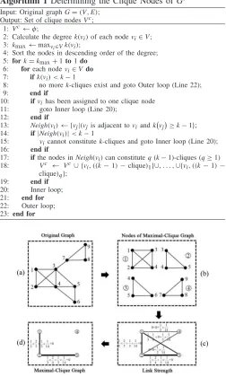
Fig. 3. Illustration of constructing the maximal-clique graph Gcfrom the original graph G. (a) Original graph G contains 9 nodes and 14 edges. (b) Clique nodes of Gccontains one 4-clique and three 3-cliques. (c) Link strength between different clique nodes is calculated and given beside each line. (d) wthris set to the averaged link strength of the graph in (c) and the
final maximal-clique graph is determined.
its neighbors (line 17). Then all the discovered k-cliques are added to the set of clique nodes (lines 18 and 19).
Figs.3(a) and (b) exemplify the above determination process of clique nodes. Fig. 3(a) shows the original graph with 9 nodes and 14 edges. The corresponding clique nodes are given in Fig.3(b), including one 4-clique and three 3-cliques. As can be seen, each node of the original graph is assigned to at least one clique node (i.e., maximal clique) of the cor-responding maximal-clique graph. For example, nodes v7, v8, and v9belong to clique node vc4, while nodes v4and v5belong to both clique nodes vc2 and vc3.
B. Measuring Link Strength Between Cliques Nodes
[image:4.612.312.564.59.479.2]Fig. 4. Examples of (a) overlapping nodes, (b) overlapping edges, and (c) joint edges.
overlapping nodes, overlapping edges, and joint edges. Given two cliques, an overlapping node is a common node of both cliques, an overlapping edge is a common edge of both cliques, and a joint edge is an edge that connects a node in one clique with a node in the other. Taking two 3-cliques as an example in Fig. 4, node v3 in Fig. 4(a) is an overlapping node, the edge between nodes v2 and v3 in Fig. 4(b) is an overlapping edge, and the edge between nodes v3 and v4 in Fig.4(c) is a joint edge. Since each clique node in a maximal-clique graph is a maximal-clique, the link strength between two maximal-clique nodes can be evaluated in the same way as evaluating the link strength between two cliques. Given two clique nodes vc
mand
vcn(m=n), the ratios of overlapping nodes, overlapping edges, and joint edges are calculated as
on
vcm,vcn
= N
vcm
vcn
Nvc m
+Nvc n
−Nvc m
vc n
(5)
oe
vcm,vcn=
vi,vj∈(vcm∩vc n)Aij
vi,vj∈VAij
(6)
je
vcm,vcn=
vi∈(vcm−vc
n),vj∈(vcn−vcm)Aij
vi,vj∈VAij
(7)
where N(vcm)and N(vcn) return the number of original nodes
in clique nodes vc
mand vcn, respectively, and N(vcm∩vcn)returns
the number of original nodes in the intersection between clique nodes vcmand vcn. A is the adjacent matrix of the original graph and Aij = 1, if (vi,vj) ∈ E; otherwise, Aij = 0. Based on
on, oe, and je, the link strength L(vcm,vcn) between vcm and
vcncan be defined as a weighted sum of these three components
Lvcm,vcn=αon
vcm,vcn+βoe
vcm,vcn+γ je
vcm,vcn (8) where α, β, γ ∈ [0, 1] are the weights that control the impact of overlapping nodes, overlapping edges, and joint edges on the link strength, respectively. Note that α+β +γ =1. In this paper, for simplicity, all the weights are set to 1/3, namely, we consider that these three parts have equal contributions to the link strength between two clique nodes. Explicitly, we can derive that L(vcm,vcn)is within [0, 1), and only if there are no overlapping nodes, overlapping edges, and joint edges between vcm and vcn, L(vcm,vcn)=0.
In Fig. 3(c), the nonzero link strength between the clique nodes in Fig. 3(b) is given. Taking the link between clique nodes vc1 and vc2 as an example, there are two overlapping nodes and one overlapping edge, but no joint edges. The total number of original nodes in clique nodes vc1 and vc2is 5. The number of original edges in G is 14. Hence, on = 2/5, oe = 1/14, and je = 0, and the link strength between vc1 and vc2 is L(vc1, vc2)=1/3(2/5+1/14+0).
C. Determining Clique Edges of Maximal-Clique Graph According to the previous two steps, the clique nodes and the link strength between them are obtained. Some links are strong, while the others are weak or even close to zero. If all the links with nonzero strength are admitted as clique edges, the following two problems may occur when detect-ing communities. First, the computational cost increases due to the large number of clique edges. Second, noise usually exists in a complex system, and thus weak links can interrupt the detection of community structure. In order to avoid the above problems, a threshold wthr is operated on the clique edges to counteract the influence of noise and lower the complexity. A link is admitted as a clique edge only if its strength is beyond wthr. The setting of wthr will be discussed in Section V-B.
After determining clique edges, the original graph G is con-verted into a maximal-clique graph Gc. The link strength is considered as the weight of the corresponding edge. Take Fig. 3(d) as an example. With wthr set as the average link strength, only two links in Fig. 3(c) are admitted as clique edges, resulting in a maximal-clique graph with four clique nodes and two clique edges.
IV. MCMOEA
This section details the implementation of the proposed MCMOEA, including the representation scheme, evolutionary operators, and the overall procedure.
A. Representation Scheme
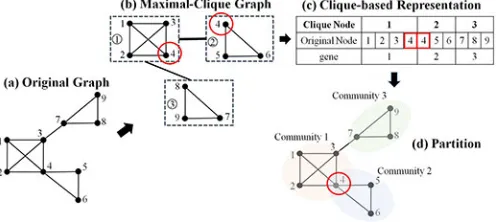
How to represent solutions in EAs has a great influence on the design of evolutionary operators and the algorithmic efficiency. As stated in Section I, the existing representation schemes, either prototype-based or node-based, have certain limitations when applied to the overlapping community detec-tion. To address these limitations, this paper proposes a new representation approach based on the introduced maximal-clique graph, namely, maximal-clique-based representation. In the proposed representation, each gene of an individual is an inte-ger that represents the community label of the corresponding clique node of the maximal-clique graph. Thus, every clique node can only be assigned to a unique community, which is similar to the separate community detection. However, as the maximal-clique graph has the property that clique nodes are allowed to share the same original nodes, the overlapping nodes shared by different clique nodes can actually be assigned to multiple communities. Taking Fig. 5 as an example, node v4 is shared by both clique nodes vc1 and vc2 [Fig. 5(b)]. Since vc1 is assigned to community “1” and vc2 is assigned to community “2” [Fig. 5(c)], node v4 belongs to both com-munities “1” and “2” [Fig. 5(d)]. The detailed population initialization is described as follows.
Let Ii=(gi1,gi2, . . . ,giM)be the ith individual in the
pop-ulation of MCMOEA, where gij is the jth gene of Ii(j =
1,2, . . . ,M,i=1,2, . . . ,PS,M is the number of clique nodes of the maximal-clique graph and PS is the size of population). The initialization of Iiis conducted by using a local algorithm
[image:5.612.85.301.334.424.2]Fig. 5. Example for the clique-based representation. (a) Original graph G. (b) Corresponding maximal-clique graph Gcis constructed based on G and each node in G is allowed to be assigned to multiple clique nodes of Gc, e.g., node v4belongs to both clique nodes vc1 and vc2. (c) Proposed clique-based
representation is adopted to assign each clique node an integer to represent the community label this node belongs to. For example, the community label of clique node vc1is 1, indicating that vc1belongs to community “1.” (d) Partition of the original graph G is directly determined based on the individual.
In detail, the algorithm builds the partition C as follows. First, the M clique nodes are randomly permuted and C is initial-ized as an empty set. Then, following the permutation order, each unassigned clique node vcm is assigned to the first com-munity whose cohesiveness can be improved by including vcm. If vcm cannot improve the cohesiveness of any existing com-munities, a new community that only contains vcm is added
to C. Considering that the maximal-clique graph is a weighted graph, the cohesiveness of a community c is measured as in [17]
F(c)= Win(c)
Win(c)+Wout(c) (9)
where Win(c) and Wout(c) are the total weights of internal edges and external edges of c, respectively. Based on the obtained partition C, the individual Ii can be initialized by
setting each gene gim as the community label of vcm in C.
The proposed clique-based representation scheme has three features. First, instead of using the original nodes, the pro-posed approach uses clique nodes (i.e., maximal cliques) as the basic unit of the representation. Since overlap is an intrin-sic property of clique nodes in the maximal-clique graph, clique-based representation enables MOEAs to handle the overlapping community detection problem in a way similar to that of the separated community detection. Second, the clique-based representation does not require decoding individ-uals in the population evolution process, which largely lowers the computational complexity of MOEAs for overlapping community detection when compared with the indirect node-based approach. Third, the clique-node-based representation scheme has no limitations on the shape of communities and needs no prior community information, making it superior to the prototype-based representation scheme.
B. Evolutionary Operators
Evolutionary operators, including crossover and mutation, are the most important components of EAs, which significantly influence the population diversity and the convergence speed. Hence, it is crucial to select appropriate evolutionary operators
for the algorithm. In this paper, to fit the proposed clique-based representation scheme, we adopt the one-way crossover operator [9] and design a new mutation operator based on the maximal-clique graph.
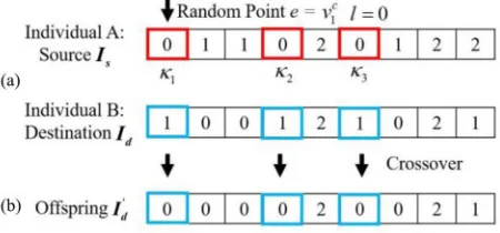
1) Crossover: In many classic EAs, the crossover operator generates offspring by randomly exchanging genes of two parental individuals [24], [35]. However, such an idea of the crossover is not suitable for the proposed clique-based rep-resentation since community labels in different individuals are not compatible. Take the two individuals A and B in Fig.6(a) as an example. According to the clique-based repre-sentation scheme, both individuals indicate that clique nodes vc1, vc4, and vc6belong to the same community, but the commu-nity label is “0” in individual A but “1” in individual B. In this case, randomly exchanging genes between the two indi-viduals can easily break the promising community structure formed by vc1, vc4, and vc6. Therefore, this paper employs the one-way crossover operator introduced in [9]. The one-way crossover randomly selects two parental individuals from the population, with one set as the source (denoted as Is), and
the other set as the destination (denoted as Id). Then a clique
node is randomly selected as the crossover seed e. Let l be the community label of e in Is and κ be the set of clique nodes
in Is that have the same community label as l. An offspring
Id is generated by modifying Id so that all the clique nodes
inκ are relabeled as l. By doing so, the offspring can merge the community structures of both parents. Using the two indi-viduals in Fig. 6(a) as parents, Fig. 6(b) shows an example of offspring generation utilizing the above one-way crossover, given that vc1is selected as the crossover seed (i.e., e=vc1and l=0). For each individual, the crossover operator is executed with a predefined possibility pc.
2) Mutation: A new mutation operator is proposed in this paper to fit the clique-based representation. The essential idea is to improve the communities with low cohesiveness by including clique nodes that have strong connections with them. In detail, for each individual Iiin the population, the mutation
operator first calculates the cohesiveness of each community in Ii according to (9). Then an M-dimensional vector ri is
generated, in which each element rij is a random number
uniformly distributed in [0, 1]. rij is compared with the
cohe-siveness of the community cgij that the clique node vcj belongs
to. If rij is larger than F(cgij), a clique node vck adjacent to
vcj is randomly selected through the roulette wheel selection. The larger the weight on the clique edge (vcj, vck), the higher the probability that vck will be selected. The mutation operator then changes the community label of vcj (i.e., gij) to that of
vck (i.e., gik). By doing so, each community in Ii, especially
the one with low cohesiveness, is given a chance to adjust its structure, which leads to a possible improvement in the overall fitness.
C. Overall Procedure of MCMOEA
[image:6.612.51.301.55.166.2]Fig. 6. Simple illustration of the one-way crossover operator. (a) Parental individuals. (b) Offspring.
community detection into several scalar optimization sub-problems. Considering that the shape of PF is unknown and the weighted sum approach only works well for concave PF, Tchebycheff approach [27] is used in MCMOEA for decomposition. Let λ1,λ2, . . . ,λPS be a set of evenly spread weight vectors, where λi = (λi1, λi2) (λi1, λi2 ∈ [0,1], and λi
1+λi2=1) and PS is the size of population (i.e., the number of subproblems). Based on the maximal-clique graph and two objective functions defined in (3) and (4), a subproblem can be formulated as
minimize gtex|λi,z∗
=maxλi1KKM(x)−z1∗, λi2RC(x)−z∗2 (10) where x is a solution to the problem, z∗=(z∗1,z∗2)is the refer-ence point, i.e., the best values found so far for the KKM and RC, respectively, and i = 1,2, . . . ,PS. MCMOEA approxi-mates the PF by minimizing the PS scalar subproblems defined above using a population with PS individuals.
As shown in Algorithm 2, MCMOEA contains three steps: 1) construction of the maximal-clique graph; 2) initialization; and 3) population evolution. In the first step, the maximal-clique graph Gcis constructed from the original graph G using the method introduced in Section III. In the second step, the population with PS individuals is initialized according to the clique-based representation scheme proposed in Section IV-A. PS weight vectorsλ1,λ2, . . . ,λPSare assigned to the PS
indi-viduals I1,I2, . . . ,IPS, respectively. Then, the neighborhood
B(i) of each weight vector is determined by Euclidean distance. The reference point z∗is initialized by the KKM and RC values of I1and the set of non-dominated solutions, NS, is initialized as an empty set. In the third step, the population is evolved through the evolution operators described in Section IV-B. A new individual z is generated by performing crossover and/or mutation on each existing individual Ii. After
evalu-ating z with the two objective functions (i.e., KKM and RC), the reference point, the neighborhood of Ii, and the set of NS
are updated accordingly.
The computational complexity of MCMOEA can also be analyzed from the above three steps. Suppose that there are N nodes in the original graph G, M clique nodes in the corresponding maximal-clique graph Gc, and the maximum node degree in G is kmax. In the first step, the computa-tional complexities of determining the clique nodes, mea-suring the link strength, and determining the clique edges
Algorithm 2 MCMOEA
Input:
G=(V,E): the original graph;
genmax: the maximum number of generations; PS: the size of population;
λ1,λ2, . . . ,λPS: a uniform spread of PS weight vectors; T: the size of the neighborhood of each weight vector; Output:
NS: the set of non-dominated solutions.
1. Construction of the Maximal-clique Graph Gc:
1) Determine the set of clique nodes Vc;
2) Measure the link strength between clique nodes;
3) Determine the set of clique edges Ecbased on the link strength. 2. Initialization:
4) Initialize the population P= {I1,I2, . . . ,IPS}, where each individual
Ii=(gi1,gi2,gi3, . . . ,giM)represents the current solution to the i-th subproblem;
5) Initialize the neighborhood of each weight vector. For each i = 1,2, . . . ,PS, set B(i) = {i1,i2, . . . ,iT}, whereλi1,λi2, . . . ,λiT are the T closest weight vectors toλiin the Euclidean space;
6) Initialize z∗as(KKM(I1),RC(I1));
7) Initialize NS as an empty set. 3. Population Evolution :
8) for g=1 to genmax
9) for i=1 to PS
10) Generate a random number rifrom U(0,1);
11) if ri<pc
12) Randomly choose another individual from B(i) and generate an offspring x by conducting the one-way crossover on this individual and Ii;
13) else
14) Set x as Ii;
15) end if
16) Generate an M-dimensional random vector rifrom UM(0,1);
17) for j=1 to M
18) if rij>F(cgij)
19) Generate a new individual z by mutating x;
20) end if
21) end for
22) if KKM(z) <z∗1, set z∗1 as KKM(z); 23) if RC(z) <z∗2, set z∗2 as RC(z);
24) for each individual Ij∈B(i)
25) if gte(Ij|λi,z∗) >gte(z|λi,z∗), replace Ijwith z;
26) end for
27) Remove from NS all the solutions that are dominated by z; 28) Add z to NS if no solutions in NS can dominate z;
29) end for
30) end for
U(0,1): the normalized uniform distribution.
are O(N×k3max),O(M2), and O(M), respectively. Hence, the computational complexity of the first step is O(max{N × k3max,M2}). In the second step, the computational complexity is bounded by the operation of population initialization which takes O(M2×PS). In the third step, the time complexity of crossover and mutation operators is related to M and can be realized in linear time, namely, O(M). The other operations can be finished in constant time. Therefore, the time complexity of the third step is bounded by O(M×PS×genmax) (PS is the size of population and genmaxis the maximum number of gen-erations). To sum up, the overall computational complexity of MCMOEA is O(max{N×kmax3 ,M2×PS,M×PS×genmax}). It should be noted that M is usually smaller than or equal to N.
V. EXPERIMENTS ANDDISCUSSION
TABLE I
PARAMETERSETTINGS OFSYNTHETICNETWORKS
thr
of the proposed MCMOEA. First, the generation model of synthetic networks and evaluation indexes in use are intro-duced. Second, the influences of the parameter wthr, evalua-tion indexes and MOEA frameworks on the performance of MCMOEA are experimentally tested. Third, the performance of MCMOEA is evaluated on synthetic networks with differ-ent characteristics and compared with other five represdiffer-entative algorithms. Finally, MCMOEA is applied to four real-world networks and the benefit of using a multiobjective framework to detect overlapping communities is illustrated.
In all experiments, the parameters of MCMOEA are set as follows. PS and genmax are set as 100 and 50, respectively [27]. The crossover probability is set as a rela-tively high value, 0.7, to increase the population diversity [27]. The neighborhood size T is set as 20 according to the sug-gestion of MOEA/D [30]. All the experiments are carried out on computers with Intel Core i5-3470 (3.20 GHz) CPU, 16 GB RAM, and Ubuntu 12.04 LTS 64-bit operating system.
A. Synthetic Networks and Evaluation Indexes
In this paper, the Lancichinetti–Fortunato–Radicchi (LFR) model [36] is adopted to produce synthetic networks. A synthetic network under LFR can be described as LFR(N,k,kmax, τ1, τ2,cmin,cmax, μ,On,Om). N is the
num-ber of nodes. k and kmaxare the average node degree and the maximum node degree, respectively. τ1 and τ2 are the expo-nents of the power law distributions that the node degrees and the community sizes, respectively follow. cmin and cmax are the minimum and the maximum size of each community. μ ∈ [0,1] is a mixing parameter that controls the average ratio of the external links to the total links of each node. If μ =0, all the edges in the network are intraconnections. If μ=1, all the edges are interconnections. Therefore, a larger μ indicates a more ambiguous community structure. On and
Om are two parameters specially defined for controlling the
overlapping rate of communities in the network. On is the
number of overlapping nodes, evaluating overlapping density among communities. Similar toμ, the higher the value of On,
the more ambiguous the community structure is. Om, namely,
overlapping membership, is the number of communities to which each overlapping node belongs. The difficulty of the detection problem increases with the rise of Om.
Once the above parameters are determined, a synthetic network can be generated from the LFR model using the method in [36]. In this paper, the settings of LFR parame-ters follow the suggestions in [27] and [37]. k, kmax,τ1, and τ2 are fixed at 20, 50, 2, and 1, respectively. N is set at three levels: 1000, 5000, and 10000. (cmin, cmax) is set as (20, 50), (30, 70), and (40, 100) at different levels of N, respectively, since the community size generally slightly increases with the scale of the network.μvaries from 0.1 to 0.5, Onvaries from
0.1N to 0.5N, and Om varies from 2 to 8. In each
experi-ment, a set of networks with different settings of N, μ, On,
and Om is considered, which is summarized in Table I. The
effectiveness and efficiency of MCMOEA can thus be studied at different levels of network scale, community ambiguity, and overlapping rate.
As a multiobjective algorithm, MCMOEA yields a set of non-dominated solutions, none of which is superior to the other on both objectives of KKM and RC. In order to facilitate comparison with algorithms that treat overlapping community detection as a single-objective problem, an evaluation index is needed to select one solution from the set of non-dominated solutions. In this paper, the generalized normalized mutual information (gNMI) [16] and the modularity (Qov) [38] are adopted as the evaluation criteria. The first index, gNMI, eval-uates the similarity between the true partition and the detected one, which is only suitable when the true community struc-ture is already known. The second index, Qov, measures the
difference between the fraction of edges within the given com-munities and the expected fraction if edges are distributed at random. Obviously, Qovcan be used without knowing the true
community structure. Therefore, gNMI can only be used in the experiments on synthetic networks, while Qov can be used on
both synthetic and real-world networks. Both gNMI and Qov
range from 0 to 1. The higher values of the gNMI and Qov
are, the better the quality of a solution will be.
B. Investigation of the Parameter wthr
yet significant influence on the algorithmic performance since MCMOEA operates on the maximal-clique graph. To study the effect of wthr and find its appropriate setting, the per-formance of MCMOEA using different wthr is compared on eight synthetic networks. For detailed settings of the synthetic networks, please refer to part 1 of Table I. On each net-work, MCMOEA is tested with wthrrising from 0 to 30wavg, where wavg is the average link strength of clique nodes in the maximal-clique graph. For each value of wthr, MCMOEA is run for 30 independent times and the average gNMI value is reported for comparison. Fig. S2 in the supplementary material, plots the average gNMI as a function of wthr/wavg.
From Fig. S2 in the supplementary material, it can be observed that in most cases the MCMOEA with extreme wthr values performs the worst, e.g., wthr = 0 or wthr =30wavg. This observation is not surprising. If wthris too small, a large number of links between clique nodes are kept as clique edges, which interferes community detection as the noise between communities increases. On the opposite, if wthris too large, most links between clique nodes are filtered out, which causes possible loss of useful information for revealing the actual community structure. Besides the above observation, it is also noticed that the curves in Fig. S2 in the supple-mentary material, have consistent shapes. That is, the average gNMI value rises from wthr = 0, reaches the top at about wthr = wavg, remains steady for a small interval, and then drops until wthr = 30wavg. Such a phenomena suggests that wthr =wavg is a generally good setting no matter what kind of network it is. Hence, the wthr is always set to wavg in the following experiments.
Comparing the curves in Fig. S2 in the supplementary mate-rial, it can also be summarized that the decreasing trend after the turning point becomes less steep asμ, On, or Omincreases.
As stated in Section V-A, larger values of μ, On, and Om
indicate a more ambiguous community structure and a higher overlapping rate. In this case, a larger wthris preferred for fil-tering out more links so that the community structure becomes clearer.
C. Investigation of gNMI and Qov
Since gNMI and Qovare both evaluation indexes suitable for
synthetic networks, an experiment is designed here to inves-tigate the differences between the partitions chosen by gNMI and Qov. To make a comprehensive test,μ, On, and Om are all
set to different levels, which are {0.1, 0.3, 0.5}, {0.1N, 0.3N, 0.5N}, and {2, 4, 6, 8}, respectively. N is set to 1000. The detailed parameter settings of the synthetic networks are listed in part 2 of Table I. On each network, MCMOEA is run for 30 independent times. For each run, the best gNMI value and the corresponding Qov (gNMI_Qov) value, as well as the best
Qovvalue and the corresponding gNMI (Qov_gNMI) value are
recorded. The average results of each index over 30 runs are reported in Fig. S3 and Table SI in the supplementary material. From Fig. S3 in the supplementary material, it can be observed that the difference between the best gNMI and Qov_gNMI, or
between the best Qov and gNMI_Qov is slight, indicating the
solutions chosen by gNMI and Qovare similar.
Additionally, to make a further comparison, this paper also examines the cumulative distributions of community sizes of partitions chosen by gNMI and Qov and compares them
with the known ground truth. The results are presented in Figs. S4–S6 in the supplementary material. As can be seen, compared to Qov, the cumulative distribution curves of gNMI
are closer to those of the true partitions on almost all net-works, implying that gNMI may be slightly more suitable as the evaluation index for synthetic networks. Therefore, in the following experiments, gNMI is used as the crite-rion on synthetic networks and Qov is used on real-world
networks.
D. Comparisons of MCMOEAs Based on Different MOEAs
As stated in Section II-C, different kinds of MOEAs are applicable for the proposed MCMOEA [39]–[43]. Therefore, in this section, except MOEA/D, other state-of-the-art MOEAs are adopted to implement MCMOEA for investigating the per-formance of MCMOEA based on different MOEAs. Among the existing MOEAs, NSGA-II [31] is a classical domination-based MOEA, which has been widely used in many fields and shown excellent performance. MOEA_DLA [33] is a new MOEA, which achieves a competitive performance by tak-ing advantages of both MOEA/D and NSGA-II. Therefore, this paper chooses NSGA-II and MOEA_DLA as the rep-resentatives of MOEAs to implement MCMOEA and com-pares their performance with MOEA/D-based MCMOEA. The implementation details of MCMOEA using NSGA-II and MOEA_DLA as the MOEA frameworks are, respectively, provided in Algorithms S1 and S2 in the supplementary material.
The parameter settings of the synthetic networks are listed in part 3.1 of Table I. To make a comprehensive compar-ison, μ, On, and Om are all set to different levels, which
are {0.1, 0.3, 0.5}, {0.1N, 0.3N, 0.5N}, and {2, 4, 6, 8}, respectively, and N is set to 1000. For the sake of fair-ness, parameters of the three MCMOEAs are set to the same values, i.e., PS = 100, genmax = 50, and pc = 0.7.
On each network, each MCMOEA is run for 30 indepen-dent times and the average gNMI is reported in Table SII in the supplementary material. Additionally, the computa-tional speed of three MCMOEAs is also compared on several networks with different scales. The corresponding network information is listed in part 3.2 of Table I. The compari-son results are reported in Table SIII in the supplementary material.
E. Experiments on Synthetic Networks
In this section, based on the synthetic networks, two exper-iments are designed to test the effectiveness and efficiency of MCMOEA. The first experiment makes a comprehensive anal-ysis of how MCMOEA performs on networks with different properties, including community ambiguity (μ), overlapping rate (Onand Om), and network scale (N). The second
experi-ment compares the performance of MCMOEA with other five representative algorithms.
1) Performance of MCMOEA on Synthetic Networks: To well observe how the performance of MCMOEA varies on networks with the change of eitherμ, On, Om, or N separately,
the method of controlling variables is adopted here. That is to say, when investigating one parameter, the other ones are held constant. Therefore, this experiment is divided into four parts. 1) Verifying the performance of MCMOEA on networks
with differentμand constant On, Om, and N.
2) Verifying the performance of MCMOEA on networks with different Onand constantμ, Om, and N.
3) Verifying the performance of MCMOEA on networks with different Om and constantμ, On, and N.
4) Verifying the performance of MCMOEA on networks with different N and constantμ, On, and Om.
In each part, to give a comprehensive result, the fixed parame-ters except N are all set to two values, which are the minimum and maximum of their feasible ranges, respectively. As for N, considering the computational cost, it is always set to 1000 in the first three parts. The detailed parameters setting of the synthetic networks is presented in part 4 of TableI. For each network, 30 independent runs of MCMOEA are conducted and the average gNMI is used as result.
First, the performance of MCMOEA on networks with dif-ferent μ is investigated. On, Om, and N are set to {0.1N,
0.5N}, {2, 8}, and 1000, respectively. Through increasing μ from 0.1 to 0.5 with the step of 0.1, the performance of MCMOEA is evaluated on each network and the results are shown in Fig. S7 in the supplementary material. As can be seen, all curves in Fig. S7 in the supplementary material, present similar tendency that the performance of MCMOEA naturally decreases with the increase ofμ, because a higher value of μ indicates a more ambiguous community structure.
Second, the performance of MCMOEA on networks with different On is evaluated. μ, Om, and N are set to
{0.1, 0.5}, {2, 8}, and 1000, respectively. The performance of MCMOEA is displayed in Fig. S8 in the supplementary material with On increasing from 0.1N to 0.5N with the
step of 0.1N. Obviously, we can see that with On increasing,
MCMOEA performs worse and worse. This is not surprising because a larger On implies a higher overlapping density, and
such a high overlapping density usually blurs the boundary of the communities and increases the challenge to the community detection.
Third, the performance of MCMOEA on networks with different Om is tested. μ, On and N are set to {0.1, 0.5},
{0.1N, 0.5N}, and 1000, respectively. Om varies from
2 to 8 with the interval 1. The results are presented in Fig. S9 in the supplementary material. As can be seen, the
performance of MCMOEA decreases with the increase of Om.
The fundamental reason is that, with the increase of Om, it
becomes harder and harder to successfully detect all the com-munities that each overlapping node belongs to, resulting in a lower partition accuracy.
Finally, we evaluate how the performance of MCMOEA changes on networks with the increase of N. μ, On, and Om are set to {0.1, 0.5}, {0.1N, 0.5N}, and
{2, 8}, respectively. N increases from 1000 to 5000 and 10000. The results are shown in Fig. S10 in the supple-mentary material. As can be seen, when μ, On, and Om
are all small, MCMOEA shows similar performance on networks with different N, such as μ = 0.1, On = 0.1N,
and Om = 2. However, when the value of μ [observing
Figs. S10(a)–(d) in the supplementary material, separately] becomes large, the performance of MCMOEA decreases with the increase of N. The similar conclusions can also be obtained on On [comparing Fig. S10(a) with (c) or
Fig. S10(b) with (d) in the supplementary material] and Om
[comparing Fig. S10(a) with (b) or Fig. S10(c) with (d) in the supplementary material]. The fundamental reason of these phenomena lies in insufficient population diversity for the large scale networks. As we know, a larger N usually means a longer length of the individual and more communities. Meanwhile, with the increase ofμ(Onor Om), the number of
communities also increases. However, for the same population size and evolutionary generation of MCMOEA, the increases of the individual length and the number of communities inevitably result in a decrease of population diversity, leading to a decrease in the quality of the final solutions.
In conclusion, we can obtain that MCMOEA works well on synthetic networks with different combinations ofμ, On, Om,
and N. For example, in Fig. S7 in the supplementary material, when On, Om, and N are set to 0.1N, 2, and 1000, the value
of gNMI is always larger than 0.85, even whenμincreases to 0.5. In Fig. S8 in the supplementary material, when μ=0.1, Om = 2, and N = 1000, the value of gNMI is larger than
0.8 even increasing On to 0.5N. Likewise, as can be seen in
Fig. S9 in the supplementary material, the value of gNMI is also larger than 0.8 even Om increases to 8 with μ = 0.1,
On=0.1N, and N =1000. Additionally, even though all the
parameters are set to the maximum of their feasible ranges, i.e.,μ=0.5, On=0.5N, Om=8, and N=10000, the value
of gNMI is still larger than 0.5 as shown in Fig. S10 in the supplementary material.
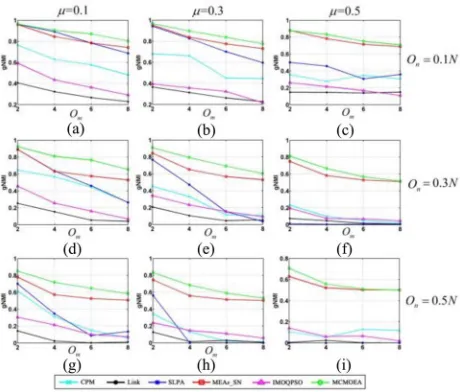
Fig. 7. Comparison results of gNMI values between MCMOEA and other five representative algorithms. (a) μ=0.1, On =0.1N, Om = {2,4,6,8}, and N=1000. (b)μ=0.3, On=0.1N, Om= {2,4,6,8}, and N=1000. (c) μ=0.5, On =0.1N, Om = {2,4,6,8}, and N =1000. (d)μ= 0.1,
On = 0.3N, Om = {2,4,6,8}, and N = 1000. (e)μ =0.3, On = 0.3N,
Om= {2,4,6,8}, and N=1000. (f)μ=0.5, On=0.3N, Om= {2,4,6,8}, and N=1000. (g)μ=0.1, On=0.5N, Om= {2,4,6,8}, and N=1000. (h) μ=0.3, On = 0.5N, Om = {2,4,6,8}, and N= 1000. (i)μ= 0.5,
On=0.5N, Om= {2,4,6,8}, and N=1000.
community detection. Link clustering [13] is featured by using links instead of nodes to discover community structures. As for SLPA [18], a previous review [37] claimed that it is a competitive method for overlapping community detection. MEAs_SN [27] and IMOQPSO [28], [44]–[47] are two rep-resentatives of MOEAs applicable to overlapping community detection. For each algorithm in comparison, the code is pro-vided by its authors. CPM, link clustering, and SLPA are implemented with C++, MEAs_SN with C, and IMOQPSO with MATLAB. The tunable parameters of each algorithm are set as the suggestion of the corresponding paper.
The parameter settings of the synthetic networks used in this section are listed in part 5.1 of TableI. In this experiment, the networks are all with 1000 nodes.μ, On, and Omare set to
{0.1, 0.3, 0.5}, {0.1N, 0.3N, 0.5N}, and {2, 4, 6, 8}, respec-tively, which are the minimum, the median and the maximum of their feasible ranges, to represent the networks with different properties. Hence, these algorithms are compared on totally 3×3×4 = 36 networks with different levels of community ambiguity and overlapping rate. By doing so, it is expected that the comparison can be comprehensive and thor-ough. For the sake of fairness, on each network, the algorithms with adjustable control parameters (i.e., CPM, link clustering, and SLPA) report their best results among different parameter settings, and the results of nondeterministic algorithms (i.e., SLPA, MEAs_SN, IMOQPSO, and MCMOEA) are averaged over 30 independent runs. The comparison results of gNMI among these algorithms are presented in Fig. 7 and Table SIV in the supplementary material. Additionally, in order to provide insight into the behaviors of different algorithms, this paper also examines the cumulative distri-bution of community sizes of each algorithm and compares
it with the known ground truth on each network. The results are shown in Figs. S11–S13 in the supplementary material.
From Fig. 7, three observations can be obtained. First, as expected, the performance of all the algorithms decreases as either of the three network parameters (μ, On, or Om)
increases. Second, MCMOEA and MEAs_SN substantially outperform CPM, link clustering, and IMOQPSO on all the total 36 networks. Comparing with SLPA, MCMOEA and MEAs_SN achieve similar performance whenμ, On, and Om
are all small. However, with either of the three parameters (μ, On, or Om) increases, the performance of SLPA decreases
dramatically and becomes much worse than MCMOEA and MEAs_SN. Third, when compared MCMOEA with MEAs_SN, MCMOEA performs better than, or at least as well as MEAs_SN on all networks. Moreover, MCMOEA is more robust to the variations of On and Om. Take the first column
of Fig.7as an example [i.e., Figs.7(a), (d), and (g)]. Withμ and Om fixed and On rising from 0.1N to 0.5N, the change of
gNMI for MCMOEA is smaller than that of MEAs_SN. Take Fig. 7(d) as another example. With μ and On fixed and Om
rising from 2 to 8, the performance of MCMOEA degrades more gently than that of MEAs_SN. From Figs. S11–S13 in the supplementary material, it can be observed that when μ, On, and Omare all small, the cumulative distributions of
com-munity sizes of CPM, SLPA, MEAs_SN, and MCMOEA are similar and close to the true community size structures. With the increase of eitherμ, On, or Om, all curves gradually
devi-ate from the known ground truth. However, compared to other algorithms, the curves of MCMOEA are closer to those of the true partitions on almost all networks.
Although MCMOEA shows great superiority in gNMI to other algorithms, recent studies [48]–[50] pointed out that gNMI may have the selection bias problem that tends to choose solutions with more communities. That is to say, a par-tition with a higher number of communities is more likely to obtain a larger gNMI value. To avoid this possible unfairness caused by gNMI, another evaluation index, called scaled nor-malized mutual information (FNMI) [49], is also adopted to evaluate the performance of all algorithms in comparison. As an adjustment of gNMI, FNMI [49] can overcome the defect of gNMI to some extent by punishing partitions that have a number of communities either too higher or too lower than the true number. Similar to gNMI, FNMI is in the range of [0, 1] and a larger FNMI represents a better partition. The com-parison results of FNMI among all algorithms are presented in Fig. S14 and Table SV in the supplementary material. From Fig. S14 in the supplementary material, it can be observed that the comparison results of FNMI are roughly similar to those of gNMI. For example, the performance of CPM, link cluster-ing and IMOQPSO are much worse than those of MCMOEA and MEAs_SN on all networks. SLPA has the similar perfor-mance to MCMOEA and MEAs_SN whenμ, On, and Omare
all small. However, with the increase of eitherμ, On, or Om, its
TABLE II
COMPUTATIONALTIME OFMCMOEAANDMEAs_SN
networks as shown in Fig. 7. However, when measured by FNMI, MCMOEA shows worse performance than MEAs_SN on networks with a larger μ. To uncover the fundamental reason of such difference, this paper examines both com-munity information of partitions obtained by MCMOEA and MEAs_SN, including the number of communities (cn), the
minimum community size (cmin), and the maximum commu-nity size (cmax), and then compares them with the known ground truth. As shown in Table SVI in the supplementary material, it can be noticed that when μ is large, cmax of MEAs_SN is much larger than that of both MCMOEA and the true partition, indicating MEAs_SN tends to merge small communities into a large one on the networks with a high value of μ. As a result, the obtained cn is decreased and its
difference with the true number of the communities is short-ened. In this case, the punishment of FNMI for the partition is alleviated, and thus MEAs_SN obtains a high FNMI value. Based on the above results, we can see that only MEAs_SN can be comparable with the proposed MCMOEA on parti-tion accuracy. However, as stated in Secparti-tion I, the indirect representation scheme adopted in MEAs_SN leads to a high computational complexity as O(N2 × PS × genmax) [27]. Nevertheless, the developed MCMOEA only costs O(max{N× k3max,M2×PS,M×PS×genmax}), which is determined by three parts, i.e., the determination process of clique nodes of the maximal-clique graph, population initialization, and evolutionary operators. Here, N is the number of nodes of the original graph, kmax is the maximum node degree of the original graph, and M is the number of clique nodes of the corresponding maximal-clique graph. PS is the size of popula-tion and genmaxis the maximum number of generations. Since M is usually smaller than or equal to N, both O(M2×PS)and O(M×PS×genmax)are much less than O(N2×PS×genmax). Thus, O(N×k3max)is the key differentiator between MEAs_SN and MCMOEA. According to the analysis of pseudo code of Algorithm 1, it can be obtained that O(N×k3max) is the worst case complexity of the clique nodes determination pro-cess. Additionally, in most large real-world networks, kmax is generally kept at 102, which is much smaller than N and does not largely increase with the rise of N.1 Therefore, the computational complexity of MCMOEA is much lower than that of MEAs_SN. Moreover, the larger the network is, the more obvious superiority of MCMOEA to MEAs_SN will be. To further validate the above analysis, an experiment is con-ducted here to compare the actual run time between these two algorithms on several synthetic networks with different scales. The detailed network information is listed in part 5.2 of Table I. On each network, MCMOEA and MEAs_SN are, respectively, run for 30 independent times with equal compu-tational budget (PS=100 and genmax=50) and the average
1snap.stanford.edu/data/.
TABLE III
INFORMATION OFTWOLARGEREAL-WORLDNETWORKS
computational time is shown in Table II for comparison. As can be seen, the computational time of MCMOEA is always much less than that of MEAs_SN when N increases from 1000 to 10,000 and the advantage of MCMOEA enlarges with the increase of N. These experimental results are consistent with the theoretical analysis of the computational complexity, which demonstrates the proposed clique-based representation is beneficial for reducing the computational cost of MOEAs for overlapping community detection. All the above observa-tions indicate that MCMOEA is a competitive and promising method for overlapping community detection.
F. Experiments on Real-World Networks
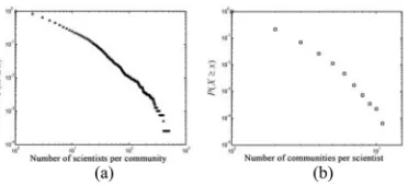
For further validation, MCMOEA is applied to detect the community structures of four real-world networks, including two small networks and two large networks. The two small networks are about word association [13], each baring one of the following two overlapping community structures: 1) two communities share multiple nodes and 2) one node belongs to several communities. The two large networks are about word association [51] and scientific collaborators [52]. The word association network was created by the University of South Florida and University of Kansas, which adopted words as stimulus and asked participants to write the first word that came into mind. The scientific collaborator network describes coauthorships between scientists that post preprints on the condensed matter E-print archive. Information about the two large real-world networks is presented in Table III. Since the actual community structures of these real-world networks are unknown, Qovis adopted as the evaluation index. Additionally,
the distributions of community sizes (nodes per community) and overlapping membership (communities per node) in large real-world networks are often found to follow power laws approximately [12]. Hence, for the two large networks, the cumulative distributions of community sizes and overlapping membership are also presented.
Fig. 8 shows an example of the partitions found by MCMOEA for the two small networks. In Fig.8(a), the parti-tion divides the network into two communities, one of which is related to “juice” and the other is related to “mixture”. “blend” and “blender” are detected as the overlapping nodes of the two communities. Such a rational partition shows that MCMOEA can deal with the situation when two communities have multiple overlapping nodes. In Fig. 8(b), the network is partitioned into four communities, each of which repre-sents one meaning of the word “brush”. “Brush” is detected as the overlapping node of the four communities. Such a parti-tion indicates that MCMOEA can also capture the community structure where one node belongs to several communities.
As for the word association network, the partition found by MCMOEA achieves a Qovof 0.15. Figs.9(a) and (b) present the