360° View Camera Based Visual Assistive Technology for Contextual Scene Information

8-2017

360° View Camera Based Visual Assistive

Technology for Contextual Scene Information

Mazin Ali

[email protected]

Follow this and additional works at:http://scholarworks.rit.edu/theses

This Thesis is brought to you for free and open access by the Thesis/Dissertation Collections at RIT Scholar Works. It has been accepted for inclusion in Theses by an authorized administrator of RIT Scholar Works. For more information, please [email protected].

Recommended Citation

Technology for Contextual Scene Information

by

Mazin Ali

A Thesis Submitted in Partial Fulfillment of the Requirements for the Degree of Master of Science

in Electrical Engineering

Supervised by

Dr. Ferat Sahin

Department of Electrical and Microelectronic Engineering Kate Gleason College of Engineering

Rochester Institute of Technology Rochester, New York

Ausgust 2017

Approved by:

Dr. Ferat Sahin, Professor

Thesis Advisor, Department of Electrical and Microelectronic Engineering

Dr. Gill Tsouri, Associate Professor

Committee Member, Department of Electrical and Microelectronic Engineering

Dr. Sildomar Monteiro, Assistant Professor

Title:

360° View Camera Based Visual Assistive Technology for Contextual Scene Information

I, Mazin Ali, hereby grant permission to the Wallace Memorial Library to reproduce my

thesis in whole or part.

Mazin Ali

Dedication

Acknowledgments

I would like to thank my parents for their endless support. For their guidance and

providing me with the chance to pursue my dreams.

I would also like to thank my advisor Dr. Sahin for his continuous support, guidance and

the trust he places on us his students, for being a great teach, mentor and most of all a

great friend.

Celal, thank you for your friendship. it has been a absolute pleasure for me to have you as

friend, a brother, a teacher and mentor. Thank you for all the times you have been there of

me, for everything you have tough me.

Finally, I would like to thank Lilian, my oldest and best friend, for her continuous support

ever since we were undergraduate, through out my masters

It has been an honor be a part of the Multi-Agent Bio-robotics Laboratory family

Abstract

360° View Camera Based Visual Assistive Technology for Contextual Scene Information

Mazin Ali

Supervising Professor: Dr. Ferat Sahin

In this research project, a system is proposed to aid the visually impaired by providing

partial contextual information of the surroundings using 360° view camera combined with

deep learning is proposed. The system uses a 360° view camera with a mobile device to

capture surrounding scene information and provide contextual information to the user in the

form of audio. The system could also be used for other applications such as logo detection

which visually impaired users can use for shopping assistance.

The scene information from the spherical camera feed is classified by identifying objects

that contain contextual information of the scene. That is achieved using convolutional

neural networks (CNN) for classification by leveraging CNN transfer learning properties

using the pre-trained VGG-19 network. There are two challenges related to this paper, a

classification and a segmentation challenge. As an initial prototype, we have experimented

with general classes such restaurants, coffee shops and street signs. We have achieved a

List of Contributions

• Implementation of a new visually assistive technology for the visually impaired.

• Use a spherical camera instead of narrow field of view camera.

• Implementation of such system with small amount of data for custom target classes.

• Comparison of the performance of Linear SVM, Quadratic SVM and Ensemble

Sub-space Discriminant classifiers over the data collected.

• Publication

Ali, M., Kumar, S., Savur, C., Sahin, F., "360° View Camera Based Visual Assistive

Contents

Dedication . . . iii

Acknowledgments . . . iv

Abstract. . . v

List of Contributions. . . vi

1 Introduction . . . 1

2 Background . . . 3

2.1 Classification Methods . . . 3

2.1.1 Support Vector Machine . . . 4

2.1.2 Ensemble Subspace Discriminant . . . 6

2.2 Convolutional neural networks . . . 7

2.2.1 Convolutional Layer . . . 9

2.2.2 Pooling Layer . . . 12

2.2.3 Fully Connected Layer . . . 14

2.2.4 Activation Layer . . . 14

2.2.5 Existing Models . . . 16

2.3 Feature Reduction . . . 17

2.4 Preprocessing . . . 19

2.4.1 Sliding Window . . . 19

2.4.2 Fish-eye Distortion . . . 19

3 Literature Survey . . . 21

3.1 Existing Object Detection Frameworks . . . 21

3.2 Transfer learning . . . 22

3.3 Feature Maps Visualization . . . 23

5.1.1 Data Augmentation . . . 31

6 Results and Discussions . . . 33

6.1 Results and Discussion . . . 33

6.1.1 System Limitations . . . 36

7 Conclusion . . . 39

7.1 Future work and Conclusion . . . 39

List of Tables

2.1 Number of the feature before and after PCA . . . 19

5.1 Dataset Composition: Class DD (Dunkin Donuts)|Class MD (McDonald’s)|Class PC (Pedestrian Crossing)|Class SB (Starbucks)|Class Null (Null) . . . 31

6.1 The Classification results of the ten classifiers with PCA. . . 34 6.2 The Classification results of the ten classifiers without PCA. . . 34 6.3 The Classification results of the ten classifiers with PCA. Using camera

List of Figures

2.1 SVM with Hard Margin hyperplane . . . 4

2.2 SVM with Soft Margin hyperplane . . . 5

2.3 Ensemble Classifier [1] . . . 6

2.4 Feedforward neural networks . . . 8

2.5 RightFeedforward neural network,LeftConvolutional neural Network [2] 9 2.6 Left to Right, fifth convolutional layer with filter number 2, number151 and number 111 activating to dogs face, human face and cat face respec-tively [3] . . . 10

2.7 Pooling operation [2] . . . 13

2.8 Max pooling [2] . . . 14

2.9 Fully connected layer . . . 15

2.10 RELU . . . 15

2.11 Sliding window going over an image frame scheme. The Figure dimen-sions are not to scale . . . 20

2.12 Pincushion Fish-eye Distortion . . . 20

3.1 General representation of convolutional neural network divided into a fea-ture extractor stage and classification stage [4]. . . 23

3.2 Activation levels of a filter output (on the Right) for person face image (on the Left) . . . 24

4.1 System Pipeline. . . 25

4.2 Raw unprocessed 360° view camera image of a Starbucks coffee shop front view. . . 26

4.3 Image de-stitching four segments . . . 26

4.4 De-stitched camera image. Left image, Front camera lens. Right image, Rear camera lens. . . 27

4.5 Top-view illustration of the field of view of each camera lens . . . 29

5.1 A sample of the segmented camera images dataset. [MD, McDonald’s : SB, Starbucks : DD, Dunkin Donuts : PC, Pedestrian Crossing] . . . 30

6.1 The confusion matrix of the Ensemble Subspace Discriminant classifier at two different trails. The axes indexing represent the class initials same as in Table 5.1. The bottom right cell shows the classifier overall accuracy. . . 36 6.2 The confusion matrix of the Linear SVM classifier at two different trails.

The axes indexing represent the class initials same as in Table 5.1. The bottom right cell shows the classifier overall accuracy. . . 36 6.3 Fish-eye lens distortion image correction, left uncorrected image, right

Chapter 1

Introduction

The International Classification of Diseases organization has visual impairment categorized

by the degree of loss of vision for an person ranging from Normal Vision to Severe Visual

Impairment and finally total Blindness. Currently, statistics estimates show that 285 million

people are visually impaired worldwide of which 39 million are totally blind and the 246

million have low vision [6].

Currently, there is a variety of assistive technology developed for visual impairment

for different degrees of vision. For example, a Dedicated Word Processor for note taking,

e-book reader such as Kindle, computer and mobile screen readers software and finally a

Refreshable Braille Displays as alternative solution to computer screen reader [7].

Existing assistive tools that addresses navigation such as white canes has been oriented

towards assisting with path sensing, obstacle detection and avoidance which is mainly

di-rected towards achieving a sense of independence for the visually impaired not

inclusive-ness in terms of spatial awareinclusive-ness. Inclusive visual information is the information obtained

by a visually un-impaired person while visually impaired persons have no access to due

to their impairment. Examples of inclusive information would be a recognition of a store

navigate around but cannot provide inclusive visual information.

Newly developed assistive technology such as the Horus wearable technology [8] and

Microsoft glasses for the blind [9] are promising prototypes for the future of assistive

tech-nology. Both prototypes provide essential functionality such as text and facial recognition

as well obstacle detection.

In this study, we propose a system that uses a 360° view camera, pre-trained neural

net-work and a linear classifier for object recognition for a set class of objects. Such system

would provide contextual information of the scene such as coffee shops street signs. The

coffee shops and restaurants are identified by their brand logos. The system would also

provide the direction of the information for localization. An example of contextual

infor-mation provided would be a "What, and Where" such as "A Starbucks coffee shop at 45

degrees to your left"

The system proposed in this paper differs from the previously mentioned prototypes by

using 360° view camera instead of a camera with a fixed field of view. The advantage of

using a 360° view camera, users are not required to turn around for object detection which

Chapter 2

Background

This chapter gives background information about the methods and algorithms used in this

study. We will present algorithms and methods for preprocessing, feature reduction, and

classification. The structure of the background starts with the classification algorithms used

in this research. Then followed by convolutional neural networks as they are used to

gen-erate the feature vector to the classifiers mentioned. Due to the data high dimensionality

feature reduction techniques are used. Finally we explore on the preprocessing that takes

places prior to feeding the input to the system proposed in section 4.

2.1

Classification Methods

The image classification problem of this research falls in the category of supervised

learn-ing. Supervised learning is a learning approach when both input and corresponding output

available at training time. The objective is to approximate a decision function that for a

given input predicts a correct output. Using a training dataset in which a training sample

is vector (feature vector) and the output is distinct label in case of classification, a

deci-sion function (hypothesis) is approximated. The measure of how a hypothesis performs on

Figure 2.1: SVM with Hard Margin hyperplane

well means it perfumes well predicting labels accurately for new data. In this research,

following Machine learning algorithms were used:

• Support Vector Machine

• Ensemble Subspace Discriminant

2.1.1 Support Vector Machine

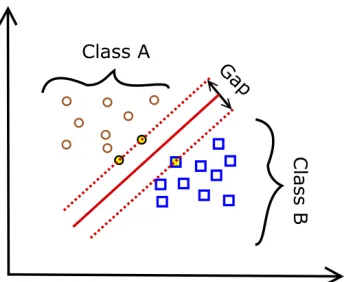
Support Vector Machine (SVM) is a supervised machine-learning algorithm. The algorithm

objective is to map the data points into a space where multi-dimensional data points are

linearly separable in the a new space. The data points are then separated into classes of

data points groups with classes most outer points names support vectors which determines

the size of the separation gap between classes as shown in Figure 2.1.

The data points such as the one used in this research are not linearly separable, hence the

space transformation into a space where the data points are linearly separable is required.

The objective is using a suitable basis function, apply a nonlinear transformation to transfer

the data points into a new space where a linear model could model the new space data points

below whereφ(x) is the basis function in equation 2.1.

g(z)=wTz g(x)=wTφ(x)

= k X

j=1

wjφj(x)

(2.1)

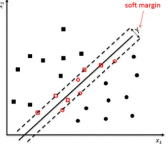
Hard margin hyperplane is used when all the transformed data points are linearly separable

shown in Figure 2.1 . In the case when the data points in the new space are not linearly

separable as shown in Figure 2.2, Soft margin hyperplane is used.

Figure 2.2: SVM with Soft Margin hyperplane

For a kernel functionK(xt,_{x), the SVM equation is written as}

g(x)= wTφ(x)= X t

αt

rtφ(xt)Tφ(x)

= X

t

αt

rtK(xt,x)

2.1.2 Ensemble Subspace Discriminant

An ensemble predictor consists of many weak learners where each learner makes a

predic-tion then vote on a predicpredic-tion amongst them as shown in Figure 6.1.

Figure 2.3: Ensemble Classifier [1]

The random subspace ensembles are used to improve the performance of the

discrim-inant analysis. The algorithm implemented on Matlab works as the following [11] where

m is the number of dimensions (variables) to sample in each learner. d is the number of dimensions in the data andnis the number of learners in the ensemble.

• Choose without replacement a set of m predictors from the d possible values.

• Using just the m chosen predictors train a weak learner.

• Repeat the previous two steps until there arenweak learners.

• Make a predict by taking the weak learners prediction average score, and classify the

and properties, as they are an essential part of this research proposed system.

2.2

Convolutional neural networks

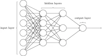
Feedforward neural networks (FNN) are an abstraction of the human brain neurons, where

each node represents a brain neuron. Mathematically, feedforward neural networks with

single hidden layer are considered universal function approximators[12]. In feedforward

neural networks, nodes connect to multiple inputs and multiple outputs through weighted

connections.The weights of these connections are learned during training.

feedforward neural networks are modeled in equation 2.3 wherewT, xand brepresent the network weights, inputs and biases respectively. The forward propagation of where the

input xiand the outputyi for single node shown in the equation 2.4.

y= f(wTx+b) (2.3)

yi = X

i

xiwi+b (2.4)

When a feedforward neural networks receives and input, it is propagated through

neu-rons in the fully connected hidden layers where each hidden layer consists of neuron

con-nected to all the neurons in the previous hidden layer. These neurons function

indepen-dently without sharing any connection with other neurons located on their layer. Figure 2.4

is basic representation of a Feedforward neural networks.

FNN’s intrinsic properties lead to inefficiency and difficulty for them to scale well on

Figure 2.4: Feedforward neural networks

if a regular neural network is used, a single neuron in the first hidden layer would have

224x224x3 = 150528 weights. Even with advances in hardware and software computa-tional powers such networks are wasteful inefficient as such large number of parameters

leads to over-fitting.

Another type of feedforward neural networks which is well suited for the tasks related

to the field of computer vision, convolutional neural networks (CNN). The main difference

between a regular feed forward neural network and convolutional neural network is that

feedforward networks node output is a multiplication of input xi and weight wi as shown in equation 2.4 while the in convolutional neural network it is a dot product between

con-volutional layer filter and the input Xi to the filter as shown in equation 2.5 as the filterF moves across the input volume.

Yi = Xi∗F =                        

a b c d e f g h i

                        j ∗                        

1 2 3

4 5 6

7 8 9                        

=(i∗1)+(h∗2)+(g∗3)+(f∗4)+(e∗5)+(d∗6)+(b∗8)+(c7)+(a∗9)

(2.5)

Due to the properties of convolutional neural networks, they are more computationally

different types of layers, convolutional layers, pooling layers, activation layers and fully

connected layers. We explore these layers in the following sections.

Recent advances in convolutional neural networks models such as AlexNet [13], VGG

(2014) [14], ResNet (2015) v[15] outperforming previous proposed algorithms to solve

problems such as image classification. Convolutional neural networks have three main type

of layers Convolutional layers, Pooling layers and Fully-Connected layers. Convolutional

neural networks differ from regular neural networks as the inputs and output are structured

in 3-D volumetric constructs with height, width and depth as shown in Figure 2.5 with each

neuron connected to a small region of the layer preceding it. The final output layer of the

convolutional neural network has output with dimension 1x1xN where N is the number of

output classes or labels.

Figure 2.5:RightFeedforward neural network,LeftConvolutional neural Network [2]

2.2.1 Convolutional Layer

The Convolutional layer consists of a set of filter. The values of these filters is the learnable

parameter of the layer. For an input image with size M xN x3 and the first convolutional layer K filters of size (Receptive Field) I xJwhere I M & J N and 3 represents the color channels. In the forward pass the filters convolve across the input image and compute

Assuming the first convolutional layer has receptive field of 3x3. For an RGB image with three color channels, each neuron will have (3x3)x3 = 27 connection weights to the input volume plus a +1 bias parameterb. Assuming as we move higher in the network a convolutional layer with receptive field of 5x5 and with input volume size 10x10x20. Every neuron in that layer will have 5x5x20 weights connecting to input volume.

The 2-dimensional activation map result of the previous process, which shows the

re-sponses of the filters at every spatial region as shown in Figure 2.6. Over the training period

the filters learns to activate to different features such as edges, patterns blobs or colors. As

we move up the network at higher layers, such filters become more discriminant to the

features activate to [3] such as a human nose a dog face. Replacing filters with large

recep-tive field with multiple smaller receprecep-tive fields results in a smaller number of parameters

to learn as well as due to the multiple activation layers such as RELU leads to a more

discriminative decision function [2].

Figure 2.6:Left to Right, fifth convolutional layer with filter number 2, number151 and number 111 activat-ing to dogs face, human face and cat face respectively [3]

In the following subsections we address two aspects of convolutional layers,

There are three main hyper-parameters to control the size of a convolutional layer output

volume, Depth, Stride and Zero-padding. Depth of an output volume is different from depth

of a network. Depth of an output volume corresponds to the number of filters in a layer and

network depth represents the number of layers in a network. In this section, the term depth

refers to the output volume depth.

Stride parameter refers to the stride by which the filter moves along an input. For

ex-ample, if a stride is set to 1 the filter will move 1at a time, if the stride is set to 5 the filter

will move 5 pixel at a time. Conventional choice of the stride hyper parameter is 2.

Zero-padding means Zero-padding zeros around the input boarder. Zero-Zero-padding is used to match

the input and output height and width. One example of matching the input and output

spatial sizes is constraining the stride S = 1 and consequently P = (F−1)/2 where Pis zero-padding andF is receptive field.

Input/Output Volume

The relationship between the input and output volumes is governed by equation 2.6,2.6

and 2.6 where the output volume of a convolutional layer given input volume with Height

Hin, WidthWin and output with Height Hout, Width Wout and Depth Dout. Setting the hy-perparamters such receptive field Hr fxWr f depth K and stride S and zero-padding P, the output volume is shown below. Hr fxWr f are representing receptive field height and width are symmetric and sometime are referred to asF as well.

Hout =(Hin−Hr f +2xP)/S +1 (2.7)

Dout = K (2.8)

It is impractical of evaluate each pixel value with different filter value. Hence, parameter

sharing is adopted by constraining the neurons in each depth slice to use the same set of

weights and bias. The example below is intended to draw a comparison with and without

the parameter sharing property. Referring to equation 2.6. Using the CNN’s architecture

with the input to the network is 227x227x3. The first convolutional layer properties of receptive field F = 11 stride S = 4, no zero-padding P = 0. Using equation 2.6, (227−

11)/4 + 1 = 55 with 96 filters k = 96 the layer output is 55x55x96. In other words 55x55x96=290400 neurons are connected to a region of size 11x11x3 of the input.

Following on the previous example, without parameter sharing, each of the 290400

neurons will have 11x11x3 = 363 weights plus+1 bias. The resultant total number of pa-rameters 290400x364 =105,705,600. On the other hand using parameter sharing, having a unique set of 96 filter weights results in a total of 96x11x11x3 =34,848 unique weights plus+96 biases.

2.2.2 Pooling Layer

Pooling layers reduce spatial size of the convolutional layers output. The main objective for

such layer is parameter and computation cost reduction-controlling over-fitting as a result.

For example pooling filter of size 2x2 and strideS =2 will down sample input by 2 along width and height while maintain the depth dimension as shown in Figure 2.7. There are

pooled likewise for Average pooling.

Figure 2.7: Pooling operation [2]

Max Pooling

Max pooling function replaces the elements of the receptive field with the element with

maximum value. The pool then moves with receptive field F by stride amount of S. Max pooling could be overlapping or non-overlapping depending on the receptive field

and stride. For example, a 3x3 receptive field with stride 3 is non-overlapping whereas 3x3 receptive field with stride 2 is overlapping. The second example dictates that for a receptive field 3x3 moves 2 steps will result in an overlap with previous receptive field. It is a common practice to use small receptive field and stride values such that the pooling

is non-overlapping. Looking at Figure 2.8, an example of a non-overlapping max pooling

with 2x2 receptive field and stride 2. Average Pooling

Similarly, to max pooling, average pooling replaces the elements of the receptive field with

Figure 2.8: Max pooling [2]

favor of max pooling since it is empirically shown to be better. Max pooling emphasis the

significant information while average pooling blurs out the details.

L2 Pooling

L2-norm equation is shown in 2.9. Similarly, to average pooling, L2 pooling replaces the

elements of the receptive field with their L2-norm value.

|X|₂=

s X

i

X_i2 (2.9)

2.2.3 Fully Connected Layer

The fully connected layers are the same layers used in the feed forward neural networks

where every neuron is connect to the all the neurons on the preceding layer as well as

following layer as shown in Figure 2.9. The fully connected layers of a convolutional

neural network behave as a classifier with convolutional layers outputs as the classifiers

input.

2.2.4 Activation Layer

Activation layers are placed after convolutional layers. The purpose of non-linear activation

functions is to introduce non-linearity to the network to handle the non-linearity properties

Figure 2.9: Fully connected layer

neural network used in this research Rectified Linear Units activation function is used for

the activation layer of the network.

Rectified Linear Unit

Rectified linear unit or RELU activation function is currently the most widely used

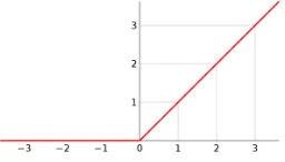
acti-vation in convolutional neural networks. Referring to Equation 2.10 and 2.11, RELU is

differentiable everywhere except at 0, also Figure 2.10 plots out functions profile.

Figure 2.10: RELU

vanishing or exploding gradient problem [16] and efficient computationally, speed of

con-vergence in comparison to Sigmoid and hyperbolic Tangent activation functions.

f(x)=                 

x, ifx>0

0, otherwise

(2.10) dy dx =                 

1, ifx> 0

0, otherwise

(2.11)

2.2.5 Existing Models

VGG-19 convolutional neural network is a 19-layers network. The network consists of a

combination of 16 convolutional layers, Maxpooling layers, 3 Fully connected layers and

an output Softmax layer [14] where all the hidden layers used RELU activation function.

The architecture of the network is sequential, meaning layers are placed in a stack form.

The convolutional neural network is among the best trained models for image classification,

wining the 2012 ImageNet challenge.

In this research the output of the VGG-19 convolutional neural network is taken right

before the first fully-connected layers, a vector of size 1x4096. The network is then con-sider as a feature extractor as the input is an RGB image and the output is feature vector

later which is further explored in section 3.2. The VGG-19 is a pre-trained network on

dimensional data. Hence the use of feature reduction techniques such the Principle

compo-nent Analysis, is explored further in the following section

2.3

Feature Reduction

Principle component analysis “PCA” is an unsupervised projection method used to reduce

data dimensionality without using the output information and variance as the criterion to

be maximized [10]. Transforming a set of related variables into a of linearly uncorrelated

set of variable called principle components “PCs” [10]. The principle components, which

refer to a set of orthonormal Eigenvectors with corresponding Eigenvalues that represent

the data variance.

Mapping inputydata point with dimensionNinto a new dimensional space with corre-sponding ˆydata point with dimensionK whereK < N with minimum loss of information. PCA application has computational advantages such as reducing training time of the

ma-chine learning algorithms as well reducing memory usages.

The mathematical application of PCA starts with orthogonal projection of the feature

vector onto the column space spanned by the Eigenvectors show in Equation 2.12

ˆ

yj =yjW (2.12)

Equation 2.12 optimal solution is obtained by Equation 2.13

W = VL (2.13)

value decomposition “SVD” matrix factorization method is used to calculate the

eigenvec-tors. Using equation 2.14 The set of feature vectorsY can be decomposed.

Y =US VT (2.14)

S is a matrix with the main diagonal containing the singular values, whereV are the right singular vectors and U are the left singular vectors. A connection between the eigenvectors

and the singular values can be made when SVD is used. In reference to Equation 2.15

and 2.16, where eigenvectors of YTY which are equivalent to V and D representing the eigenvalues ofYTY which is equal to the squared singular valuesS,D= S2.

YTY =VSTUTUS VT =V(STS)V = V DVT (2.15)

(YYT)V =V D (2.16)

The selection of eigenvectors VL from the truncated SVD using a rank L approximation withLrepresenting the minimum number of eigenvalues whose sum isp% of the total sum of all eigenvalues as shown in Equation 2.17

L=argmax

l        l l X

i=1

D(i,i)₆tr(D).p

       (2.17)

Finally, referring to equation 2.13 whereW as PCA matrix, using equation 2.12 to project the feature vectors into a new subspace with lower dimensionality. PCA is applied in this

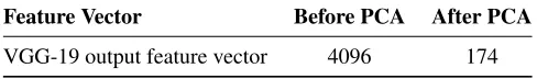
research on the convolutional neural network output feature vector. The feature vector is of

Feature Vector Before PCA After PCA

VGG-19 output feature vector 4096 174

2.4

Preprocessing

Initially the image recieved from the 360 view camera is stitched resulting a 2866x5376. The image then is destitched into two equal size image frames, Front and Rear camera

im-age. The images are then cropped vertically along the Y-Axis using only the top 40% of

the image as no valuable data with regards to this study is found at the bottom 60% of the

image.

2.4.1 Sliding Window

The serch for objects in an image frames is carried out by running a sliding window over

the image frame. An image frame is a 2688x2688 pixels, and the sliding window is of size 1000x1000. The sliding window starts at the top left corner of the image frame then move along the X-axis with jump increments of 500 pixels. The same jump increments are used

for moving long the Y-axis shown in Figure 2.11. The result is a total of 8 sliding windows

per image frame (front or rear) meaning 16 sliding windows per a 360 view image.

2.4.2 Fish-eye Distortion

The Ricoh Theta S fish-eye lens has a pincushion distortion. One the properties of the

pincushion distortion is it is minimum at the center of the image frame, as shown in Figure

Figure 2.11: Sliding window going over an image frame scheme. The Figure dimensions are not to scale

image. On the left is the full frame image of the Rear camera lens [C], and on the right, is

the segmented image that is used during training and testing [D].

Chapter 3

Literature Survey

This chapter presents a literature review of the characteristics of convolutional neural

net-works that allows for using them for the implementation of contextual scene information

extraction using object detection frameworks.The structure of the of this chapter starts of

with a review over the existing state of the art object detection framework. But unlike in

the previous mentioned frameworks, due to the scarcity of training data, we take advantage

of some of the Convolutional neural networks properties such as transfer learning.

3.1

Existing Object Detection Frameworks

Existing object detection frameworks such as Regions with VGG-16 CNN “R-CNN” [17]

which uses regions proposals to segment the image then run it through the CNN. A better

performing framework was proposed, Fast R-CNN which changed the method by which

the regions proposals are processed by projecting the regions proposals on the feature map

generated by the CNN convolutional layers prior to the fully connected layers [18]. The

author of [18] then proposed a new system named it Faster R-CNN [19] which differed from

Fast R-CNN by introducing a Region Proposal Network “RPN” to generate proposals more

accurately. It is faster since the RPN network is embedded in the image classification CNN

computational cost. Although the Faster R-CNN is a single network it is considered a part

framework. You Only Look Once “YOLO” is another object detection framework in which

the object detection problem is defined as a regression problem [20]. Similarly, Single Shot

multi-box Detector “SSD” framework shares the single network single evaluation attribute

as the YOLO but differs by using a set of default bounding boxes sizes [21].

3.2

Transfer learning

Pre-trained neural networks learn new tasks within the same domain faster than training

a new neural network from scratch. Transfer learning of a convolutional neural networks

that trained on Chinese text to retrain on Latin text is possible because they both share the

same text language domain [22]. A trained convolutional neural network can be considered

a two-stage pipeline process as shown in Fig 3.1.

(i) Feature Extraction Stage:

All convolutional layers up to the fully connected layers block can be considered as

a feature extractor. examples of features the convolutional neural network could be

sensitive to are objects textures, colors or edges.

(ii) Classification Stage:

All the remaining fully connected layers can be considered as the classifier.

Convolutional neural networks learn similar general filters after training on natural images

datasets regardless of the cost function [23]. The reason behind that is the shared domain

in terms of the nature of images the networks trained on. Hence the possibility of transfer

Figure 3.1: General representation of convolutional neural network divided into a feature extractor stage and classification stage [4].

a base task to be used for a new task of similar nature. Given that the learned filters are

general for both the base and the target tasks. Transferring learned filters is done by

ini-tially freezing weights updates of the convolutional layers during back-propagation, while

allowing for the last fully connected layers to update its weights during retraining over a

new training data.

3.3

Feature Maps Visualization

Visualizing the feature maps of a convolutional neural networks provides better insight and

results in better understanding of them. One of the ways to visualize a feature map is to

map out the output image of a feature map for a specific image input as shown in figure

2.6. The author in [24] states that feature maps are not random or un-interpretable but

rather show a change in invariance as well as class discrimination as one ascends in the

convolutional layers. It is shown that there is a greater invariance at the higher layers as

well as an emphasis of discriminative segments of the image.

level of activation of a filter output for an image input. Comparing both the activation

output and the image shows the correlation between the level of activation and the

cor-responding objects in an image frame. The level of activation depends on object present

in an image frame as well as the specific filter. Finally, the convolutional neural network

shows activation channels that are sensitive to faces of people and animals after training

on ImageNet, a dataset with no dedicated face class but contained image classes with faces

in them [3] as shown in Fig 3.2. The figure is an illustration of visualizing a feature map

using activation levels of a filter output. The test image shown is taken from the ImageNet

dataset. For more examples and information refer to the paper Understanding Neural

Net-works Through Deep Visualization [3]

Chapter 4

Proposed Method and Experiments

The system setup consists of the 360° view camera, a Wi-Fi connectivity module and a

processing unit which in this experiment for convenience a laptop is used. The 360° view

camera is dual fisheye lens spherical camera. The images are stitched internally by the

camera to provide the 360° view. The multi-stage system pipeline process is shown in

Figure 4.1. The work-flow goes as the following:

Figure 4.1: System Pipeline.

(i) Wireless Communication

An API call made to the camera to take an image with default dimension 2688x5376.

The communication between the camera and computer is set up to ve over wifi. The

command messages sent from the computer are packages inJSONformat.

(ii) A second API call commands the camera to send the image over Wi-Fi.

The Ricoh Theta S is a dual lens camera. Each lens is a hemispherical lens. The

is received and viewed in panoramic mode "Equirectangular" shown in Figure 4.2.

Using the image in Figure 4.2 for examples illustration in the following steps.

Figure 4.2: Raw unprocessed 360° view camera image of a Starbucks coffee shop front view.

(iii) Image preprocessing

The received stitched image is first decoupled. The decoupling in this research is

im-plemented by initially dividing the stereo image into four segments with size 2688x1344 as shown in Figure 4.3. The four segments nameA, B, C, Dare rearranged to the

re-sult in Figure 4.3.The rear lens camera image consists of the two middle segmentsB

&C. while the front lens camera requires horizontally concatenating segmentD&A

as shown in Figure 4.4.

lenses images shown in Figure 4.4 which results in Front and Rear images sizes of

2688x2688.

Figure 4.4: De-stitched camera image. Left image, Front camera lens. Right image, Rear camera lens.

(iv) Sliding window

A sliding window of size scans over each of the front camera lens and rear camera

lens images. The sliding window has the properties discussed in section 2.4.1. The

size of the sliding window is 1000x1000.

(v) Image processing

The sliding window output image is of size 1000x1000 but it has to be downsized to a 224x224. The reason is the maximum input image size the VGG-19 network allows is 224x224.

(vi) VGG-19

The VGG-19 network is used as a feature extractor by removing the last three fully

of size 4096.

(vii) Feature reduction

Due to the high dimensionality of the feature vector, a PCA is used to reduce the

dimensionality while maintaining 95% variance. The PCA output is then used as

input for the linear classifier. In this experiment the PCA reduced the size of the

feature vector from 4096 to 174

(viii) Classification

Finally after classification, the information is converted into audio form. The

infor-mation conveys both contextual inforinfor-mation and location of the inforinfor-mation source.

(ix) Localization

Using the index of the sliding window, the location of the object with-respect-to the

agent is determined. As mentioned in section 2.4.1, the sliding window generates

a total of 8 window images per Front/Rear image. Looking at Figure 2.11 we can

determine at what angle is the object is located. The angle ranges are as shown in

Figure 4.4.

A top-view illustration of the field of view of each camera lens is shown in Figure 4.5.

With the users as the center with facing forwards as direction at 0° while Left is at

-90° and Right is at 90°.

Chapter 5

Dataset

5.1

Dataset compilation

The target classes for this system are Dunkin Donuts and Starbucks coffee shops,

McDon-ald’s restaurant and Pedestrian crossing street sign as shown in Figure 5.1. A non-object

class called the Null class which consisted of images which does not include any of the

target classes.

Figure 5.1: A sample of the segmented camera images dataset. [MD, McDonald’s : SB, Starbucks : DD, Dunkin Donuts : PC, Pedestrian Crossing]

Due to the lack of datasets for such classes of objects, two manually labeled datasets were

compiled from two different sources. The first source was the result of Google image

searches and manually labeling it.

Pedestrian crossing street sign using the Ricoh Theta S spherical camera. The sizes of the

datasets is shown in Table 5.1.

Table 5.1: Dataset Composition: Class DD (Dunkin Donuts)|Class MD (McDonald’s)|Class PC (Pedestrian Crossing)|Class SB (Starbucks)|Class Null (Null)

Class Class DD Class MD Class PC Class SB Class Null

Camera Images 121 116 120 120 122

Online Images 232 232 232 232 232

A set of relevant dataset to our research whether in objective of object detection and

localization and the nature of the target classes. With regards to the nature of target classes

the FlickrLogos-32 dataset [26] consists 8,240 images of 32 classes where each class

con-sists of images containing a logo of a brand representing a class. The previous mention

frameworks mentioned 3.1 trained on datasets such as the PASCAL VOC 2012 dataset

which consists of 11,530 training images of 20 classes [27] and the Imagenet DET [28]

dataset containing 45,6567 training images of 200 classes.

Looking the previous two datasets collecting more data is essential for the future of this

work to expand its scope of classes and functionality.

5.1.1 Data Augmentation

Image data augmentation was utilized to increase the train pool of the camera images.

It consisted of images of the target object at different locations in the image frame. An

example of the data augmentation carried out shown in Figure 5.2 of a single pedestrian

Chapter 6

Results and Discussions

This chapter presents results of the experiments for the proposed system. Experiments are

performed with the Ricoh Theta S spherical camera based on the system proposed in

Chap-ter 4.

6.1

Results and Discussion

Training and testing on the Online compiled images dataset was a proof of concept of

the capability of the VGG-19 combined with a linear classifier to address the classification

challenge for this paper. After positive results, camera compiled image dataset was created.

The images used from the camera compiled dataset were post segmentation. The camera

image dataset was divided into 2:1 training and testing data ratio respectively.

The Classification results of the ten classifiers after training and testing on camera image

dataset shown in Table 6.1. The results are reported after 10 trails were training data was

shuffled randomly. The mean test accuracies as well as the standard deviation are calculated

accordingly. PCA is applied on the data used to train and test the classifiers in table 6.1.

The PCA had 174 principle components.

Table 6.1: The Classification results of the ten classifiers with PCA.

Classifier Accuracy % STD

linear Support Vector Machine 87.83 2.4 Quadratic Support Vector Machine 87.76 2.2 Cubic Support Vector Machine 85.7 2.7 Fine Gaussian Support Vector Machine 24.0 1.6 Linear Discriminant Analysis 83.9 2.9

Fine K-Nearest Neighbor 51.2 6.2

Ensemble Bagged Trees 72.4 3.9

Ensemble Boosted Trees 65.6 4.2

Ensemble Subspace K-Nearest Neighbor 71.5 2.9 Ensemble Subspace Discriminant 85.3 2.1

data on the same ten classifiers previously mentioned but without applying PCA.

Compar-ing the results on table 6.1 and 6.2, results show the performance increase introduced when

using PCA.

Table 6.2: The Classification results of the ten classifiers without PCA.

Classifier Accuracy % STD

linear Support Vector Machine 83.1 2.0 Quadratic Support Vector Machine 82.7 2.5 Cubic Support Vector Machine 80.7 2.8 Fine Gaussian Support Vector Machine 20.9 0.5 Linear Discriminant Analysis 70.9 3.1

Fine K-Nearest Neighbor 69.4 2.6

Ensemble Bagged Trees 71.6 4.5

Ensemble Boosted Trees 68.1 4.6

Ensemble Subspace K-Nearest Neighbor 74.9 3.0 Ensemble Subspace Discriminant 80.0 2.6

The results indicates that the data high dimensionality is counterproductive such that

when we reduced the data’s dimensionality using PCA, the accuracy increased as a result.

Finally, to test the possibility of augmenting new data sources as the camera training

images are not abundant, we trained the ten classifiers using the camera images and tested

using the online compiled images. The results of the experiment shown in table 6.3. We

use PCA to reduce the data dimensionality and increase accuracy as shown in 5.1 and 6.2.

Classifier Accuracy % STD linear Support Vector Machine 59.4 5.6 Quadratic Support Vector Machine 58.7 5.1 Cubic Support Vector Machine 57.1 5.7 Fine Gaussian Support Vector Machine 20.0 0.0 Linear Discriminant Analysis 57.7 3.8

Fine K-Nearest Neighbor 35.7 5.3

Ensemble Bagged Trees 48.0 4.6

Ensemble Boosted Trees 47.8 4.7

Ensemble Subspace K-Nearest Neighbor 48.2 3.0 Ensemble Subspace Discriminant 61.3 3.6

accuracy when trained and tested on camera images, it is not definitively considered the

best choice of classifier to be used for this system nor the same could be said about

En-semble Subspace Discriminant classifier. That is due to its performance fluctuations over

the pedestrian crossing class which has the highest priority due to the safety concern that

comes with it.

The confusion matrix shown in Figure 6.1 shows the Ensemble Subspace Discriminant

classifier performance of the classifier when tested on camera images. The figure shows

the Ensemble classifier with initially with 100% accuracy on pedestrian crossing class as

shown on the confusion matrix on the left in Figure 6.1. When data was reshuffled before

training testing again the classifier misclassified a Dunkin donuts as pedestrian crossing

sign once shown on the confusion matrix on the right.

although the Linear SVM classifier has a higher mean-per-class accuracy as shown in

Figure 6.2 the same case of performance fluctuations applies to it. Initially the classifier

misclassified a Null class where non of the target classes present as pedestrian crossing

Figure 6.1: The confusion matrix of the Ensemble Subspace Discriminant classifier at two different trails. The axes indexing represent the class initials same as in Table 5.1. The bottom right cell shows the classifier overall accuracy.

classier with 100 % accuracy on pedestrian crossing as shown in the confusion matrix on

the left.

Figure 6.2: The confusion matrix of the Linear SVM classifier at two different trails. The axes indexing represent the class initials same as in Table 5.1. The bottom right cell shows the classifier overall accuracy.

6.1.1 System Limitations

A common challenge of utilizing offthe shelf 360° view cameras including the Ricoh Theta

S spherical camera is the lack of availability of the proprietary intrinsic camera

character-istics information which is vital for fish-eye lens distortion correction. Hence, no lens

below in Figure 6.3.

Figure 6.3: Fish-eye lens distortion image correction, left uncorrected image, right corrected image

The figure shows that attempting to estimates the correction parameters to compensate

for the lens distortion lets to information loss or distortion as evident and could be see

by comparing the top section of the images. The information at the top of the image as

mentioned previously, is essential for our system as most of the valuable information for

this system is found at eye level or above.

On average, the time taken for image capture then data transfer from the camera to

the computer over Wi-Fi or USB takes 7 seconds on average. The bottleneck is not the

type connection but the rather the camera internal image processing. A real-time camera

feed at high resolution is available but unusable without the intrinsic camera characteristics

information for lens distortion correction. The time taken for classification is 1.5 seconds

on average. Computation time can be improved significantly by using a GPU instead of a

CPU due to the parallelizable nature of CNN computations .

connection insures longer operation time as it is only limited by the battery of the

com-puting embedded device. In addition, the USB connection has higher data transfer speeds

over Wi-Fi. On the other hand, a USB connection for the camera is at the bottom next to

the mount slot as shown in Figure 6.4 which will require a mounting mechanism redesign.

Finally, a USB connection could limit the user movement. In contrast, Wi-Fi connection

offers far greater mobility over USB as well as offering no constraints on mounting

mech-anisms. On the other hand, the user will have a shorter operation period as they will be

limited by the camera’s battery. The camera’s battery lasts for 260 snapshots with an image

capture and transfer over Wi-Fi every 30 seconds which means it can stay ON for two hours

approximately.

Chapter 7

Conclusion

7.1

Future work and Conclusion

Classification performance on camera compiled image dataset does achieve its objective

recognizing the target classes with satisfactory accuracy. As a current work in progress, we

are experimenting with training our own convolutional neural network for this classification

problem. A total of 8-layers network which is less than half the size of the VGG-19 in terms

of depth, which makes it less computationally expensive. The objective behind designing

our own relatively small size network is final product deployment. Considering deploying

such system as mobile system, challenges such as computational power requirements must

be addressed since it designed to be used as a pseudo-real time system. NVidia currently

has the Jetson TX which can be a viable solution for system mobile deployment. Designed

as a low energy consumption embedded device with enough computational power suited

for deep learning related computations [29].

Future work will include adding more functionality by adding a road clearance target

class. Current traffic lights pedestrian crossings include the accessibility functionality in

their design, using audio Beeps to aid and notify visually impaired individuals of road

which is the case at pedestrian crossings that are not at a traffic light i.e. at inner

resi-dential communities which is one of the system target classes. Hence, one of the future

complementary capabilities of the system is to notify the visually impaired user of road

clearance at pedestrian crossing street signs. Also as the system is used to detect the logos

of the store, extending the application of this system to be used indoor is a important part

of future development.

One could assume, the indoor application of this system would be of great benefit for a

visually impaired person, being able to locate a store or recognize a product brand. Hence

as an integral part of the future work, is include international brands and stores logo for

indoor use.

Finally, augmenting a GPS system to the system in this research to work as a double

check on the predictions make could enhance the accuracy and improve the user

Bibliography

[1] C. Savur, “"american sign language recognition system by using surface emg signal,” Master’s thesis, Rochester Institute of Technology, 2015.

[2] A. Karpathy, “Cs231n convolutional neural networks for visual recognition.”

[3] J. Yosinski, J. Clune, A. M. Nguyen, T. J. Fuchs, and H. Lipson, “Understanding neural networks through deep visualization,”CoRR, vol. abs/1506.06579, 2015. [4] “PARsE|Education|GPU Cluster|Efficient mapping of the training of Convolutional

Neural Networks to a CUDA-based cluster.”

[5] “Product,” March 2017.

[6] “Visual impairment and blindness,” Aug 2014.

[7] S. Robitaille, The illustrated guide to assistive technology and devices: tools and gadgets for living independently. Read How You Want, 2010.

[8] J. Beckett, “Wearable device for blind people could be a life changer |nvidia blog,” Oct 2016.

[9] “Microsoft cognitive services - wearable glasses for the visually-impaired.”

[10] Ethem Alpaydin,Introduction to Machine Learning. The MIT Press, 3rd ed., 2014. [11] “Ensemble methods.”

[12] K. Hornik, “Approximation capabilities of multilayer feedforward networks,”Neural Netw., vol. 4, pp. 251–257, Mar. 1991.

[13] A. Krizhevsky, I. Sutskever, and G. E. Hinton, “Imagenet classification with deep con-volutional neural networks,” in Advances in Neural Information Processing Systems 25(F. Pereira, C. J. C. Burges, L. Bottou, and K. Q. Weinberger, eds.), pp. 1097–1105, Curran Associates, Inc., 2012.

[15] K. He, X. Zhang, S. Ren, and J. Sun, “Deep residual learning for image recognition,”

CoRR, vol. abs/1512.03385, 2015.

[16] S. Hochreiter, “The vanishing gradient problem during learning recurrent neural nets and problem solutions,” Int. J. Uncertain. Fuzziness Knowl.-Based Syst., vol. 6, pp. 107–116, Apr. 1998.

[17] R. B. Girshick, J. Donahue, T. Darrell, and J. Malik, “Rich feature hierarchies for ac-curate object detection and semantic segmentation,”CoRR, vol. abs/1311.2524, 2013. [18] R. B. Girshick, “Fast R-CNN,”CoRR, vol. abs/1504.08083, 2015.

[19] S. Ren, K. He, R. B. Girshick, and J. Sun, “Faster R-CNN: towards real-time object detection with region proposal networks,”CoRR, vol. abs/1506.01497, 2015.

[20] J. Redmon, S. K. Divvala, R. B. Girshick, and A. Farhadi, “You only look once: Unified, real-time object detection,”CoRR, vol. abs/1506.02640, 2015.

[21] W. Liu, D. Anguelov, D. Erhan, C. Szegedy, S. Reed, C.-Y. Fu, and A. C. Berg, “Ssd: Single shot multibox detector,” 2016. To appear.

[22] D. C. Cire¸san, U. Meier, and J. Schmidhuber, “Transfer learning for latin and chinese characters with deep neural networks,” in 2012 International Joint Conference on Neural Networks (IJCNN), 2012.

[23] J. Yosinski, J. Clune, Y. Bengio, and H. Lipson, “How transferable are features in deep neural networks?,”CoRR, vol. abs/1411.1792, 2014.

[24] M. D. Zeiler and R. Fergus, “Visualizing and understanding convolutional networks,”

CoRR, vol. abs/1311.2901, 2013.

[25] A. Krizhevsky, V. Nair, and G. Hinton, “Cifar-10 (canadian institute for advanced research),”

Recognition Challenge,”International Journal of Computer Vision (IJCV), vol. 115, no. 3, pp. 211–252, 2015.