Algorithms for detecting dependencies and rigid subsystems for CAD

Accepted Manuscript

Algorithms for detecting dependencies and rigid subsystems for CAD

James Farre, Helena Kleinschmidt, Jessica Sidman, Audrey St. John, Stephanie Stark et al.

PII: S0167-8396(16)30081-4

DOI: http://dx.doi.org/10.1016/j.cagd.2016.06.001

Reference: COMAID 1575

To appear in: Computer Aided Geometric Design

Received date: 1 October 2015 Revised date: 13 April 2016 Accepted date: 10 June 2016

Please cite this article in press as: Farre, J., et al. Algorithms for detecting dependencies and rigid subsystems for CAD.Comput. Aided Geom. Des.(2016), http://dx.doi.org/10.1016/j.cagd.2016.06.001

Highlights

• Review of foundations for “body-and-cad” frameworks of CAD systems. • Detailed case study for “body-and-cad” frameworks of CAD systems. • Combinatorial “pebble game” algorithm for detecting generic dependencies.

Algorithms for detecting dependencies and rigid

subsystems for CAD

James Farrea,1, Helena Kleinschmidtb, Jessica Sidmanb,2, Audrey St. Johnb,3, Stephanie Starkb,4, Louis Theranc,5, Xilin Yub,6

a_{Department of Mathematics, University of Utah, Salt Lake City, USA} b_{Mount Holyoke College, South Hadley, MA USA}

c_{School of Mathematics and Statistics, University of St Andrews, Scotland}

Abstract

Automated approaches for detecting dependencies in structures created with Computer Aided Design software are critical for developing robust solvers and providing informative user feedback. We model a set of geometric constraints with a bi-colored multigraph and give a graph-based pebble game algorithm that allows us to determine combinatorially if there are generic dependencies. We further use the pebble game to yield a decomposition of the graph into factor graphs which may be used to give a user detailed feedback about dependent substructures in a specific realization of a system of CAD constraints with non-generic properties.

Keywords: sparsity matroid, pebble game algorithm, cad constraints

1. Introduction

In this paper, we present graph-based algorithms for analyzing and decom-posing the underlying combinatorial structure of a system of geometric

con-$_{An extended abstract of this article appeared as “Detecting dependencies in geometric}

constraint systems” in the 10th International Workshop on Automated Deduction in Geometry (ADG 2014), Coimbra, Portugal, 2014.

Email addresses: [email protected](James Farre),[email protected] (Helena Kleinschmidt),[email protected](Jessica Sidman),[email protected] (Audrey St. John),[email protected](Stephanie Stark),

[email protected](Louis Theran),[email protected](Xilin Yu) 1_{Partially supported by NSF DMS-0849637.}

2_{Partially supported by NSF DMS-0849637 and the Hutchcroft fund.}

3_{Partially supported by the Clare Boothe Luce Foundation, NSF DMS-0849637, NSF} IIS-1253146 and the Hutchcroft fund.

4_{Partially suppored by the Mount Holyoke College Lynk Program.}

5_{Partially supported by the European Research Council under the European Union’s} Sev-enth Framework Programme (FP7/2007-2013) / ERC grant agreement no 247029-SDModels, Academy of Finland (AKA) project COALESCE, and the Hutchcroft fund.

straints, such as those appearing in popular constraint-based Computer Aided Design (CAD) software. While a generic (essentially random) realization of a given system of constraints may be rigid, a specific realization may be in aspecial positionwhich admits internal motions and contains (redundant) dependencies. In such a situation, our decomposition allows us determine which subsystems of constraints remain independent and which are causing the dependencies.

1.1. Motivation

CAD software allows engineers to create designs using intuitive geometric constraints. When a user adds a constraint that is dependent, the resulting system isover-constrained. To provide useful feedback, efficient approaches are required to detect the minimal sub-system containing the dependency.

Figure 1 shows an example of a system of geometric constraints on 3 bodies constructed in SolidWorks. BodiesA andB are constrained to lie on the hori-zontal line; bodiesAandC are constrained to lie on the vertical line; there are two distance constraints between points on bodiesB andC. Together these 3 geometric constraints impose 6 independent conditions on the degrees of free-dom of the system of 3 bodies, making thebody-and-cad frameworkgenerically rigid.

A problem may arise if a specific realization of a system of geometric con-straints has special features that imply a dependency that is not present gener-ically. Commercial CAD software, such as SolidWorks, is unreliable when pre-sented with such aflexible special position. Figures 1(b) and 1(c) show a special realization of the system. Here, a dependency arises because the two point-point distance constraints betweenB andC are along parallel lines. SolidWorks’ 2D and 3D environments produce different analyses. Although the 2D Sketch en-vironment does identify the system as “Under Defined,” the faded position in 1(b) was only found by suppressing the dependent constraint, investigating the motion, then unsuppressing it.

Our ultimate goal is to be able to reliably identify such special dependencies that arise in more complicated constraint systems in terms of the geometry of the constraints as above, e.g., to be able to inform the user that the non-generic behavior is due to the fact that two bars are parallel.

1.2. Related work

Rigidity theory is applicable to a wide variety of systems of geometric con-straints. For example, in bar-and-joint rigidity theory, constraints are specified by fixing the distance (“bar”) between pairs of points (“joints”) and can be rep-resented by quadratic equations. In body-and-bar rigidity theory, fixed-length bars are attached to rigid bodies at flexible joints. The rigidity models of 2D bar-and-joint and d-dimensional body-and-bar are well-known for having com-binatorial characterizations ofgenerically rigid frameworks.

A

C B

(a) SolidWorks’ 2D Sketch environment identifies the rigidgenericembedding as “Fully Defined.’

C B A

C

B

(b) SolidWorks’ 2D Sketch environment identifies the flexiblespecial position as “Under Defined,” but does not allow the user to explore the resulting motion.

(c) SolidWorks’ 3D Assem-bly environment gives a different identification of “Over Defined” for the same flexible special posi-tion embedded in 3D.

Figure 1: Changing a constraint in a generically rigid system to be dependent (by making the dashed distance constraint parallel to the other distance constraint) results in a flexible special position.

instead focuses oninfinitesmal rigidity, which is defined in terms of the rank of a matrix obtained by linearizing the constraint equations. As a matrix drops rank on a closed set, almost every framework with the same combinatorics is infinitesimally rigid (and therefore rigid).

Infinitesimal rigidity theory may be studied numerically or combinatorially. One may detect generic dependencies numerically, by picking random realiza-tions. This is the approach taken by the “witness method” of [4]. The draw-back of numerical methods is that fast, stable, algorithms, such as SVD, do not identify the support of a minimal dependency while those based on Gaussian elimination are not stable. (This can be overcome by using finite fields and the Schwartz Lemma, as discussed in [5].)

rigidnucleation-free graphs[14].

Our approach combines the traditional combinatorial counting techniques with the connections to algebra introduced by White and Whiteley. White and Whiteley define thepure condition of a body-and-bar framework, a polynomial obtained from taking the determinant of the rigidity matrix in [15]. They showed how to interpret the irreducible factors combinatorially and how to describe some special positions using synthetic geometry via the Grassmann-Cayley al-gebra. In this paper we extend their philosophy to systems with additional types of constraints where the connections between the algebraic and combinatorial substructures associated to the constraint system are more intricate.

1.3. Contributions

We present algorithms for detecting dependencies in CAD systems modeled as body-and-cad frameworks. The first is a pebble game algorithm that can check forgeneric dependencies via the combinatorial property from [7]; when a constraint is determined to be dependent, we additionally detect itsfundamental circuit (minimal set of constraints involved in the dependency). To adapt the pebble game to our setting, the algorithm needs to partition the edges in a graph and maintain (a, a)-sparsity on one part and (b, b)-sparsity on the other; this may require dynamically adjusting the partitions.

As we saw in Figure 1, a framework that is rigid with no generic dependen-cies, orgenerically minimally rigid, may be in a flexible special position caused by the special geometry of its realization. Since a special position is indicated by the vanishing of a polynomial called a framework’spure condition, we de-velop algorithms for finding graph minors, which we refer to as factor graphs, corresponding to its factors. In the body-and-bar setting of [15], irreducible factor graphs correspond to irreducible minimally rigid subframeworks; their corresponding factors can be expressed as the pure condition of those subframe-works. However, in our setting, we may have irreducible factors that do not have a natural interpretation as the pure condition of any subframework. Yet, the ability to associate combinatorial structures to the factors of the pure condition could give a user additional tools to analyze a system of constraints.

1.4. Organization

We begin with an introduction to body-and-cad rigidity theory in Section 2. In Section 3, we analyze a framework and geometric conditions that lead to special positions, motivating the algorithms for finding generic dependencies (Section 4) and factor graphs for assisting with analysis of special positions (Section 5). We end with conclusions and open questions in Section 6.

2. Background

2.1. The combinatorial model

A body-and-cad framework consists of n full-dimensional bodies with pair-wisecoincidence,angular, ordistance constraints between them; thesecad con-straints are specified betweengeometric elements which are affine linear spaces (e.g., a point, line or plane in 3D) rigidly affixed to the bodies.

The allowed motions of a body-and-cad framework are continuous motions of the bodies that preserve the given constraints. A body-and-cad framework is rigidwhen all of the allowed motions are trivial, i.e., they consist of applying the same rigid-body motion to each of the bodies; otherwise it isflexible. Note that our model of these systems of constraints is given solely in terms of collections of affine spaces affixed to the rigid bodies and we do not consider the geometry of the body in our analysis; only special properties of the constraints affect our analysis. (For example, any special symmetries thebodies themselves may have does not enter the analysis; however, special symmetriesof the constraints do.) There are 9 different constraint types in 2D and 21 in 3D. Examples of constraints in 2D are: point-point distance(a bar),point-line coincidence, point-line distance, line-line coincidence, and line-line angular. Each geometric constraint represents one or more equations restricting the relative motion of the bodies involved. A constraint can then be further decomposed into primitive constraints, which correspond to single equations. Let dbe the dimension of the ambient space. Primitive constraints come in two types, which require distinct algebraic treatment: ablind constraint can potentially restrict any of thed+1₂ relative degrees of freedom, while anangularconstraint restricts only thed₂relative rotational degrees of freedom. Haller et al. [16] show how to coordinatize infinitesimal Euclidean motions by ad+1₂ -dimensional vector in such a way that an angular constraint involves onlyd₂of the variables.

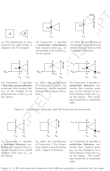
Example 2.1. To give some intuition about body-and-cad rigidity, consider the planar body-and-cad framework in Figure 2. It is composed of two rigid bodies A (the square) and B (the triangle); placing three cad constraints, a point-line coincidence,line-line perpendicularandpoint-line distance, results in agenerically minimally rigid(Definition 2.5) framework.

Now consider the framework in Figure 3; it is composed of the same two rigid bodies as in Figure 2, but only includes two cad constraints, a line-line distanceandpoint-line distance. Because Constraint I (line-line distance) is equivalent to Constraints 1 and 2 (point-line coincidence and line-line perpendicular), this system of constraints is equivalent to the figure in Figure 2 and isgenerically minimally rigid.

A

B

(a) The framework is com-posed of two rigid bodiesA

(square) andB(triangle).

_A1 p_B1

(b) Constraint 1 specifies

a point-line coincidence

that requires point p_B1 on the triangle to lie on line_A1

on the square.

_A1 p_B1

(c) After the specification of Constraint 1, the framework allows internal motion with 2 degrees of freedom.

_A1 p_B1

_{B2 A2}

_A2

(d) Constraint 2 specifies aline-line perpendicular constraint that requires line

_B2 on the triangle to be perpendicular to line_A2on the square. _A1 p_{1 B2 A2 A2}

(e) After the specification of Constraints 1 and 2, the framework allows internal motion with 1 degree of free-dom.

_A1 p_B1

_{B2 A2}

_{A2 A3}

p_B3

(f) Constraint 3 specifies a

point-line distance

con-straint that requires point

p_B3 on the triangle to be a fixed distance from line_A3

on the square. The result-ing framework is minimally rigid.

Figure 2: A generically minimally rigid 2D body-and-cad framework.

_{A1 B1}

(a) Constraint I specifies a line-line distance con-straint that requires line_B1

on the triangle to be a fixed distance from line _A1 on the square.

A1 B1

(b) After the specification of Constraint I, the frame-work allows internal motion with 1 degree of freedom.

_{A1 B1 A3}

p_B3

(c) Constraint II specifies a

point-line distance

con-straint that requires point

p_B3 on the triangle to be a fixed distance from line_A3

on the square. The result-ing framework is minimally rigid.

A B

point-line coin line-line perp point-line dist

A B

(a) Thecad graph(top) for the framework in Figure 2 has three edges between the vertices for bodiesAandB. Theline-line perpen-dicularconstraint is associated to a primi-tive angular constraint, so theprimitive cad graph(bottom) has one red edge.

A B

line-line dist point-line dist

A B

(b) The cad graph(top) for the framework in Figure 3 has two edges between the ver-tices for bodiesAandB. Because the line-line distanceconstraint is associated to two primitive cad constraints (one blind, one an-gular), theprimitive cad graph(bottom) has three edges.

Figure 4: Combinatorics of body-and-cad frameworks in Figures 2 and 3: bothcad graphs (top) are associated to the sameprimitive cad graph(bottom).

Definition 2.2. Aprimitive cad graphis abi-colored graphG= (V, E=RB) on vertex set[n] ={1, . . . , n}with a vertex for each rigid body, a red edge (inR) for each angular constraint, and a black edge (inB) for each blind constraint.

In the rest of this paper, we will work with primitive cad graphs.

2.2. The rigidity matrix and infinitesimal rigidity.

As is standard in the field, we will linearize the geometric constraint equa-tions and consider infinitesimal rigidity. Here, the core object of study is a rigidity matrix (derived in [16]), whose kernel consists of the infinitesimal mo-tions of the framework.

To describe body-and-cad rigidity matrices combinatorially, we use the fol-lowing concept7.

Definition 2.3. For integersa, b, letk=a+b. We define an[a, b]-frameG(p) to be a bi-colored graph G= (V, E =RB) with n=|V| and|E| =kn−k, along with a function p : E → Rk_{. The function p labels each edge with a}

k-vector, which is zero in the last b entries if the edge is in R. The generic [a, b]-frame G(x) has formal indeterminates replacing the nonzero coordinates ofp.

We define the rigidity matrix in terms of [a, b]-frames. We first fix some ordering on the edges ofG.

Definition 2.4. Therigidity matrixM(G(p))of an [a, b]-frameG(p)is a ma-trix that haskcolumns for each vertexiand one row for each edge ofG. In the

row corresponding to an edgee with endpoints i andj (where i < j), we have p(e)in the columns corresponding to i,−p(e)in the columns corresponding to j, and zeroes in all other entries. Order the rows of the rigidity matrix in the order of the edges ofG.

Definition 2.5. We say that an[a, b]-frameG(p)isgenerically minimally rigid if the associated generic [a, b]-frame G(x)has a rigidity matrix M(G(x)) with rankkn−k.

The generic rigidity matrix for the example in Figure 3 is shown below.

⎛ ⎝

A₁ A₂ A₃ B₁ B₂ B₃

line-line distance (blind part) x₁ x₂ x₃ −x₁ −x₂ −x₃

line-line distance (angular part) y₁ 0 0 −y₁ 0 0

point-line distance (non-generic) z₁ z₂ z₃ −z₁ −z₂ −z₃

⎞ ⎠

It has 3 columns for each body, corresponding to the one rotational and two translational degrees of freedom for instantaneous rigid body motion in the plane. We order the columns so that they are in groups of 3, with translational components last: column A₁ corresponds to the rotational component, and columns A₂ and A₃ to the translational components, with body B’s columns ordered analogously. There is a row for each primitive constraint; notice that the row for the primitive angular constraint associated to the line-line distance constraint (highlighted in red) has zeroes in the columns corresponding to the translational degrees of freedom.

While the rank of a generically minimally rigid framework is kn−k for almost all realizations, there are realizations for which the rank drops. These correspond to non-generic realizations, or special positions, of the generically minimally rigid graph.

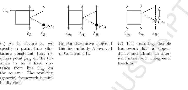
Example 2.6. In Figure 5 we construct a special position of the framework specified by the graph from Figure 3. By changing the placement of the line on bodyA in Constraint II, the resulting framework remains flexible. Its rigidity matrix is shown below8and contains a dependency (the third row is the sum of the first two), causing its rank to drop.

⎛ ⎝

A₁ A₂ A₃ B₁ B₂ B₃

point-line coincidence 1 0 −1 −1 0 1

line-line perpendicular −1 0 0 1 0 0

point-line distance (non-generic) 0 0 −1 0 0 1 ⎞ ⎠

3. Motivating case study

In this section we analyze in detail the 2D body-and-cad framework consist-ing of 3 bodies, 2 bars, and 2 line-line coincidence constraints depicted in Figure

_{A1 B1 A3}

pB3

(a) As in Figure 3, we specify a point-line dis-tance constraint that re-quires pointp_B3 on the tri-angle to be a fixed dis-tance from line _A3 on the square. The resulting (generic) framework is min-imally rigid.

_{A1 B1 A3}

pB3

(b) An alternative choice of the line on bodyAinvolved in Constraint II.

_{A1 B2 A3}

p_B3

(c) The resulting flexible framework has a depen-dency and admits an inter-nal motion with 1 degree of freedom.

Figure 5: A flexible special position of a generically minimally rigid 2D body-and-cad framework.

1. This case study will help motivate the two algorithms that we will subse-quently present that detect generic dependencies (Algorithm 1 in Section 4) and find factor graphs for dependencies arising in special positions (Algorithm 4 in Section 5).

The associated primitive cad graph, in which an edge corresponds to a linear constraint, is given in Figure 6(a). In this graph, each line-line coincidence is represented by two edges: a red edge that corresponds to a line-line parallel constraint (which restricts only angular motion) and a black edge that corre-sponds to a point-line coincidence constraint (which restricts one translational degree of freedom). Each bar eliminates 1 degree of freedom and is represented by a black edge.

Since the framework is in 2D, we will work with the generic rigidity matrix associated to the [1,2]-frame using edge labelsa, b, c, d, e, f:

⎛ ⎜ ⎜ ⎜ ⎜ ⎜ ⎜ ⎝

A₁ A₂ A₃ B₁ B₂ B₃ C₁ C₂ C₃

a₁ a₂ a₃ 0 0 0 −a₁ −a₂ −a₃

b₁ 0 0 0 0 0 −b₁ 0 0

c₁ 0 0 −c₁ 0 0 0 0 0

d₁ d₂ d₃ −d₁ −d₂ −d₃ 0 0 0

0 0 0 e₁ e₂ e₃ −e₁ −e₂ −e₃

0 0 0 f₁ f₂ f₃ −f₁ −f₂ −f₃

⎞ ⎟ ⎟ ⎟ ⎟ ⎟ ⎟ ⎠

A d B

C

a e f

c b

(a) The primitive cad graph for the frame-work in Figure 1. Red edges represent angular constraints.

1

2

A

C

B

C

C

C

C

B

(b) The special position in which₁₂.

1

2

A

B

C

(c) The special position in which the bars are parallel.

Figure 6: A 2D body-and-cad example on 3 bodies; we assume that bodyC is tied down.

As we will see in Section 5, it is convenient to work with a polynomial called the pure condition that captures the rank of the rigidity matrix. We imagine immobilizing bodyC, which has the effect of removing the last three columns of the rigidity matrix. The determinant of what remains gives the pure condition and may be expressed as thebracket polynomial[abc][def]−[abd][cef], where thebracket[abc] denotes the 3×3 determinant of the matrix whose rows are a, b and c. This pure condition is not identically zero, which is expected since the framework is generically minimally rigid. Since special positions arise when the rank of the rigidity matrix drops, these occur precisely when the pure condition vanishes. We are particularly interested in identifying subsystems where a dependency occurs, motivating the study of the factors of the pure condition.

A special position occurs when a factor of the pure condition vanishes. To give a geometric interpretation of the vanishing of the factors, we must first explain how the edge labels are obtained. We adopt the projective geometry setting of [15], so that the framework is realized (as a set of bodies) in the affine patch ofP2 that has coordinates [1 :x: y]. This apparent complication is justified by the fact that infinitesimal Euclidean motions are then naturally identified with points in (P2)∗. Since the infinitesimal constraints implied by the edge labels are, essentially, blocked motions, we interpret them as points in (P2)∗as well, allowing us to study their geometry as a point configuration. (See [15] and also [16] for a detailed treatment and the specific construction.)

factorsb₁, c₁, a₂d₃−a₃d₂, and e₂f₃−e₃f₂, whose vanishing characterize the special positions of this framework.

The next conceptual step is to relate the vanishing of the irreducible factors of the brackets derived above to our projective geometry setup. First note that since b = [b₁ : 0 : 0] is a point in (P2)∗, b₁ cannot be zero. Therefore, if [abd] =b₁(a₂d₃−a₃d₂) = 0 then (a₂, a₃) =λ(d₂, d₃) for some nonzeroλ.

The pointa∈(P2)∗ determines a line inP2; we can think ofaas a vector in R3 _{that is normal to a plane that projectivizes to a line inP}2_{.The intersection} of these two lines in P2 (respectively, planes in R3), is given by a system of equations represented by the matrix

a₁ a₂ a₃ d₁ d₂ d₃

Assuming that a= d, ifa₂d₃−a₃d₂ = 0 this is equivalent to a system of

equations of the form

1 0 0

0 d₂ d₃

.

In other words, the intersection of the lines inP2corresponding toaanddis a point of the form [0 :−d₃:d₂], which is a point on the line at infinity. Two lines meet at a point on the line at infinity if and only if they are parallel. Hence, we can conclude that [abd] vanishes when the lines₁and₂ which are denoted by₁ and ₂ in Figure 6(b)are parallel. The analysis for the vanishing of the irreducible factors of [cef] is analogous; there is a special position when the lines determined by the barseandf are parallel, as in Figure 6(c).

As this case study shows, finding the factors of the pure condition can pro-vide information about the subframeworks of a framework in a special position that contain a dependency. The algorithm that we will present in Section 5 (Algorithm 4) finds a canonical set of graph minors, which we refer to asfactor graphs, associated with the factors of the pure condition; for this example, it pro-duces factor graphs associated with precisely the irreducible factors described above, as depicted in Figure 9.

4. Detecting generic dependencies with [a, b]-sparsity

We review the notion of [a, b]-sparsity, used to characterize body-and-cad rigidity, and present the [a, b]-pebble game algorithm, which characterizes [a, b]-sparsity and consequently addressesgeneric body-and-cad rigidity. If the addition of an edge results in a dependency in a generic realization of the system, the pebble game will find its fundamental circuit (minimal set of constraints involved in the dependency).

4.1. The combinatorics of minimally rigid graphs

Theorem 1. An [a, b]-frame with bi-colored graph G = (V, E = R B) is generically minimally rigid if and only if∃B ⊆B such that:

• (V, R∪B) is the edge-disjoint union ofatrees, and

• (V, B\B) is the edge-disjoint union ofb trees

Theorem 1 can also be stated in terms ofhereditary sparsity, which we now recall. A multigraph G = (V, E) is (k, )-sparse if every subset of n vertices spans at mostkn−edges; if in addition,Ghas exactlykn−edges, it is called (k, )-tight. For brevity, (k, )-tight graphs will be called (k, )-graphs. A subset of vertices ofGthat induces a (k, )-graph is a (k, )-block. When ∈[0,2k), (k, )-graphs are the bases of the (k, )-matroid[9].

Definition 4.1. Let G= (V, E =BR)be a bi-colored graph, a, bbe positive integers, andk=a+b. ThenGis[a, b]-sparse9 _{if∃B⊆B such that:}

• (V, R∪B) is(a, a)-sparse, and

• (V, B\B) is(b, b)-sparse

Additionally, ifGhas exactlykn−ktotal edges, thenGis[a, b]-tightand referred to as an[a, b]-graph.

A subset of vertices of an [a, b]-sparse graph that induces an [a, b]-graph is an [a, b]-block.

That this class is matroidal follows from the Matroid Union Theorem [17, Prop. 7.6.14]. Therefore, for an [a, b]-sparse graph G= (V, E) and an edge e

not inE, we will say thateisindependentofGifG+eis also [a, b]-sparse and dependentotherwise.

A straightforward application of the Nash-Williams and Tutte Theorem [18, 19] implies that generic minimal rigidity of body-and-cad frameworks is characterized by [1,2]-sparsity in the plane and, omitting point-point coinci-dence constraints, [3,3]-sparsity in 3D [7].

4.2. Pebble games for[a, b]-sparsity

Algorithm 1 describes our [a, b]-pebble gamefor solving theDecision, Ex-traction, Components and Optimization algorithmic problems described in [9] for [a, b]-sparse graphs as well as detecting the fundamental circuit of a dependent edge. This algorithm belongs to a family of pebble game algorithms [20, 9] that are based on a set of local moves applied to the edges of a directed graph, where the edges and vertices are covered by pebbles representing de-grees of freedom. The specific preconditions for each type of move, which are related to the sparsity parameters, determine the sparsity family recognized by the game.

Algorithm 1The [a, b]-pebble game algorithm.

Input: A bi-colored graphG= (V, E =RB), with redRand blackB edges. Output: [a, b]-sparsity property tight, sparse, dependent and contains spanning tight, ordependent.

Setup: Initialize an empty directed graph H on vertex setV. On each vertex, placeaaqua pebbles andb tan pebbles.

Allowed moves:

Add red edgeij [Precondition: ≥a+ 1 aqua pebbles oni andj.] – Add the new edge, cover it with an aqua pebble from i (there is one by the precondition).

– Orientij out ofi.

Add black edge ij [Precondition: ≥ a+ 1 aqua pebbles on i and j or

≥b+ 1 tan pebbles oni andj.]

– Add the new edge; cover it with a pebble from i using aqua (if there are a+ 1 aqua) or tan (if there areb+ 1 tan).

– Orientij out ofi.

Edge reversal[Precondition: vertexj has a pebble on it and an in-edge

ij covered by the same color.]

– Reverse the edge by orienting it asji out of j, covering with the pebble fromj and returning the (same color) pebble originally coveringij toi. Aqua exchange edge reversal[Precondition: vertexjhas an aqua peb-ble on it and a black in-edge ij covered by a tan pebble; i and j do not belong to the same (a, a)-component of aqua pebble covered edges.] – Reverse the edge by orienting it as ji out of j, covering with the aqua pebble fromj and returning the tan pebble originally coveringij toi. Tan exchange edge reversal[Precondition: vertexjhas a tan pebble on it and a black in-edgeij covered by an aqua pebble;iandjdo not belong to the same (b, b)-component of tan pebble covered edges.]

– Reverse the edge by orienting it asjiout ofj, covering with the tan pebble fromj and returning the aqua pebble originally coveringij toi.

Method:

1. For each edgee∈E

(a) If e is black: attempt to collect b+ 1 tan pebbles on its endpoints with Alg. 2.

(b) If Alg. 2 returnstrue: insertewith anadd black edgemove. (c) Else, or if e is red: attempt to collect a+ 1 aqua pebbles on its

endpoints with Alg. 2.

(d) If Alg. 2 returnstrue: insertewith anadd black/red edgemove. (e) Else: reject it and highlight the edges returned by Alg. 2 as the fundamental circuit of the edge (if e is black, this is the union of both calls to Alg. 2).

2. If every edge is added: output tight if there are a+b pebbles left and sparseotherwise.

Algorithm 2The subroutine for finding pebbles for the [a, b]-pebble game. Input: An [a, b]-pebble game configuration (a directed bi-colored graph), an edgee, and a desired additional pebble colorc_e (aquaortan).

Output: trueif a+ 1 aqua (ifc_e is aqua) or b+ 1 tan (if c_e is tan) pebbles can be collected on the endpoints ofeorfalseotherwise, along with the set of visited edges.

Method:

1. Initialize setF =∅.

2. Initialize queue Q=∅. Entries ofQ will be of the form (f, c), recording an edge on which to cover with a pebble of colorc.

3. Sete.predecessor= NIL. 4. Enqueue (e, ce) into Q.

5. WhileQis not empty (a) Dequeue (f, c).

(b) Iff =eandf is red, continue to the next iteration of the loop. (c) Use the basic pebble game rules to try to collecta+ 1 (ifcisaqua)

orb+ 1 (ifc istan) pebbles on the endpoints off; letF be the set of edges visited by that search.

(d) If the pebbles were collected i. Letg=f.

ii. Whileg.predecessor= NIL

A. Letdbe the color of the pebble coveringg,dbe the opposite color,uandvthe source and target ofg.

B. Collect a pebble of colordonvusing the basic pebble game rules withedge reversalmoves.

C. Perform ad exchange edge reversalmove to reverse the edge fromv tou, covering it with thed-colored pebble and releasing ad-colored pebble back ontou.

D. Setg=g.predecessor.

iii. Collecta+ 1 (if cis aqua) or b+ 1 (if c istan) pebbles on the endpoints ofg(=e).

iv. OutputtrueandF∪F. (e) Otherwise

i. For each edgeg∈F that is not in F

A. Setg.predecessor=f; letcbe the opposite of colorc.

B. Enqueue (g, c) intoQ.

One way of intuitively understanding the [a, b]-pebble game is to imagine separate (a, a)- and (b, b)- pebble games played on setsAandT, which partition the current edge set, respectively. The aqua-colored pebbles track the edges in

Aas well as the (a, a)-sparsity of that partition; the tan-colored pebbles do the same forT with (b, b)-sparsity counts10. The [a, b]-pebble game relies on moves that permit black edges to move betweenAandTin a controlled manner, which corresponds to collecting additional pebbles of certain colors, using a subroutine described in Algorithm 2. To find a sequence of these moves, Algorithm 2 specializes Knuth’s matroid union algorithm [21] to the [a, b]-sparsity matroid using pebble games. By enqueuing unvisited edges (inF\F), it uses a breadth-first approach to find the shortest path (stored withpredecessor pointers) to an edge whose pebble color can be exchanged. To help illustrate the algorithm, Figure 7 shows some steps of the pebble game.

4.3. Correctness

We show correctness of Algorithm 1.

Theorem 2. A bi-colored graph is [a, b]-sparse if and only if it can be con-structed with the[a, b]-pebble game.

We are going to prove that Algorithm 1 correctly characterizes [a, b]-sparse graphs and that it can be used to find circuits. As mentioned above, we rely on Knuth’s algorithm for matroid union [21] (see [22, Sec. 42.3] for a modern treatment). Before giving the details, we remark that Knuth’s algorithm is a meta-algorithm that relies on calls to independence oracles for the two matroids underlying the union. Here, these two matroids are the (a, a)- and (b, b)-sparsity matroids, with appropriately chosen ground sets. Thus, we could simply apply Knuth’s scheme using the (a, a)- and (b, b)-pebble games as the oracles, instead of developing the [a, b]-pebble game and showing it simulates Knuth’s search procedure. However, the [a, b]-pebble game presented here saves a factor of

O(n) over the more na¨ıve approach, as we will see in the complexity analysis. Nonetheless, Lemma 4.2, below, follows from Theorem 3 and the proof of Lemma 4.3, so the direct argument below is meant to be informative.

In what follows, we describe a pebble game configuration as (H, A, T), where

H is a bi-colored directed graph on vertex set V, with a pebble covering every edge and some free pebbles on vertices; A is the set of edges covered by aqua pebbles andT is the set of edges covered by tan pebbles. We will also abuse notation slightly and use the same symbols H, A, and T to describe their underlying undirected graphs. Finally, we will use the notationS+eto denote

S∪ {e}andS−eto denote S\ {e}.

Lemma 4.2. The underlying graph of any pebble game configuration is [a, b] -sparse withA as an(a, a)-sparse graph and T as a(b, b)-sparse graph.

A B

C e

x y _z g f

(a) The input is a primitive cad graph with 5 black (solid) edges and 1 red (dashed) edge.

(b) The setup stage placesa= 1 aqua (cir-cular) pebble andb= 2 tan (square) pebbles on each vertex.

(c) Since there were at leastb+1 = 3 tan peb-bles on its endpoints, the black edge e is inserted with anadd

black edgemove.

(d) Another add

black edge move

inserts the edge f. While the direction is arbitrarily chosen, a pebble from the source is used to cover the edge.

(e) Since there were

a+ 1 = 2 aqua peb-bles on its endpoints, the red edge g is in-serted with an add

red edgemove.

(f) A few moves later, an aqua edge

exchange reversal

move is possible:

B has an aqua

pebble and a tan pebble covered black in-edge z, whose endpoints are not in a (1,1)-component.

(g) The edge z is subsequently reversed, covered by the aqua pebble fromB, releas-ing a tan pebble onto

C.

(h) Finally, all edges are successfully in-serted with exactly

a + b = 3 pebbles remaining; the output istight.

Figure 7: The [a, b]-pebble game (Algorithm 1) played on a primitive cad graph for a generi-cally minimally rigid framework determines that it is [1,2]-tight.

Proof. We show something slightly stronger, which is that the underlying graph

H constructed by applyingany sequence(as opposed to only the ones found by the algorithm) of the pebble game moves is always [a, b]-sparse.

The key invariant is that, after any sequence of moves,AandT both induce pebble game configurations for the basic (uncolored) pebble game from [9]. As an immediate consequence, we obtain thatA remains (a, a)-sparse and B

remains (b, b)-sparse. This certifies thatH is [a, b]-sparse. The invariant clearly holds at initialization, so we proceed by induction on the number of moves.

For the inductive step, we first consider all the moves except for the ex-change edge reversalmoves. We observe that, assuming the required pre-conditions, these operate entirely on either A or T as a configuration, so the inductive step for them follows directly from [9].

edge ij ∈ T is not in an (a, a)-component of A, implies that A+ij is (a, a )-sparse. From this, the pebble game invariants of [9] imply that there are a

aqua pebbles (distinct from the one onj) reachable fromivia paths using only edges in A. By induction, A could have been built by the basic (a, a)-pebble game; thenij could be added toAby basic pebble game searches. Notice that returning the tan-colored pebble toj maintainsT as a basic (b, b)-pebble game configuration.

The other direction is captured by the following lemma.

Lemma 4.3. If an edge is independent of the underlying graph of a pebble game configuration, then the pebble game will successfully insert it.

Before giving the proof, we briefly review Knuth’s algorithm and establish some terminology, specialized to our setup. The algorithm operates on a di-rected, bipartite graph associated with a pebble game configuration (H, A, T) and an edgee, which is not in H. This graph, denoted ΓH+e, has vertex set

given by the edges ofH, i.e.,AT,along with twoterminalverticesαandτ, and an additional vertex for the edgee. First, we describe the edges originating and terminating at a vertexx /∈ {e, α, τ}.

There is a directed edge from vertexxtoy, written x→yif ⎧

⎨ ⎩

(A−y) +xis (a, a)-sparse ifx∈T &y∈A

(T−y) +xis (b, b)-sparse ify∈T &x∈A∩B, i.e.,

xis a black edge in the aqua partition

Additionally, there is an edgex→α ifx∈ T and A+xis (a, a)-sparse, and there is an edge fromx→τ ifx∈A∩B andT+xis (b, b)-sparse. The edges originating ateare defined similarly. This case distinction is simply to make it clear that no edges in Γ_H+ehave eas their target.

A path x₀ → x₁ → · · · → x_π has a shortcut in a graph if there exists a

j > i+ 1 such thatxi→xj is an edge. In particular, ifx0→x1→ · · · →xπ is

a shortest path in a graph, it does not have a shortcut.

Given a path from eto a terminal vertex, recoloring along the path means puttingxi in the part of the partition containingxi+1, withαalways inAand

τ always inT.

The main result of [21], again specialized for our setup, is:

Theorem 3. Let (H, A, T) be a pebble game configuration and e an edge not in the underlying graph. Then there is a directed path inΓH+e from e toαor

τ if and only ifH+eis independent. Moreover, given a path e=x₀ →x₁→ . . .→xπ ∈ {α, τ} in ΓH+e that does not have a shortcut, a partition of H+e

certifying[a, b]-sparsity can be found by recoloring along this path.

The proof of Lemma 4.3 amounts to showing that Algorithm 2 is simulating Knuth’s algorithm.

in collecting enough pebbles on the endpoints ofe. This is done by comparing the pebble search procedure in Algorithm 2 to Knuth’s algorithm.

First consider, in the main loop of Algorithm 2, the conditional block predi-cated upon whena+ 1 (ifcis aqua) orb+ 1 (ifcis tan) pebbles can be collected on the endpoints off. Note thataaqua orbtan pebbles can always be collected on any vertex by [9]. The additional pebble can be collected if and only if the edge f can be moved to the opposite part of the partition without violating sparsity. This is equivalent to there being an edgef → {α, τ}in ΓH+e.

Otherwise, the pebble search fails. In this case, [9] implies that F +f is the fundamental circuit off in thec-colored part of the partition; i.e.,g∈F if and only if there is an edgef →g in ΓH+e. Therefore,F is exactly the set of

neighbors off in ΓH+e.

By enqueuing those edges in F not already inF, Algorithm 2 is, in fact, searching Γ_H+e in a breadth-first fashion. By Theorem 3, the assumption that

H+eis [a, b]-sparse implies that there is a path frometo a terminal vertex in Γ_H+e. Therefore, Algorithm 2 will be able to collecta+ 1 aqua orb+ 1 pebbles on the endpoints of some edge f, implying that there is an edge from f to a terminal in Γ_H+1. Let pbe the path in Γ_H+e defined by following predecessor pointers fromf. Since Algorithm 2 implements breadth-first search on Γ_H+e,p

is shortcut free.

Theorem 3 then implies that recoloring along p preserves the (a, a)- and (b, b)-sparsity of A and T at every step. The main results of [9] then imply that it will always be possible to meet the preconditions of theexchange edge reversalmoves to implement the recoloring by using only basic pebble searches onAor T. Thus, the pebble game moves implementing the recoloring alongp

will succeed, and the [a, b]-pebble game will inserte.

4.4. Circuits

The pebble game also detects [a, b]-circuits, an approach that is perhaps less well-known, but appears before in [9, Section 6] and has been used in [23]. Note that the presence of red edges creates the possibility of many types of circuits. Some may be circuits as uncolored (a+b, a+b) graphs, others may be (a, a )-circuits, and there are yet other types. The examples in Figure 8 demonstrate a property of circuits that does not arise in the (k, )-sparsity matroids. While every (k, )-circuit is (k, )-spanning, or “rigid,” an [a, b]-circuit may actually be “flexible.” Dropping an edge of a (k, )-circuit always results in a tight graph, but dropping an edge of an [a, b]-circuit can result in a sparse (but not tight) graph.

Whenever we fail to insert an edge, Algorithm 2 finds its fundamental circuit.

Lemma 4.4. Let F be the set of edges returned by Algorithm 2. The funda-mental circuit ofe in the configuration graphH isF+e.

Proof. We must show thatF+eis dependent and that, for anyy∈F,F+e−y

x z f

h e

g y

(a) The fundamental [1,2]-circuit for rejected edgeg detected by the pebble game is the set of edges{e, g, y}. The set{e, y}forms an angularly rigid block.

x z f

h e

g y

(b) The fundamental [1,2]-circuit for rejected edgeydetected by the pebble game is the set of edges{e, g, x, y, z}. The set{x, z}forms a contextually rigid block due to the presence of the angular block{e, g}.

Figure 8: Unlike (k, )-circuits, removing any edge from a [1,2]-circuit may not produce a [1,2]-graph.

from ein the Knuth graph ΓH+e. By the definition of F, every directed path

in ΓH+ethat starts ateis contained in ΓF+e. Therefore, there is no path from

eto a terminal in ΓF+e, and Theorem 3 implies thatF+eis not [a, b]-sparse.

Now, lety∈F. By construction ofF,yis on a short-cut free directed path starting at e. Therefore, there is an x ∈ F +e on this path with x → y an edge of ΓH+e.By definition, removingyresults in an edge fromxto a terminal,

providing a path frometo a terminal. In other words,F+e−y is [a, b]-sparse for ally∈F, which completes the proof of correctness.

4.5. Complexity analysis

The running time of Algorithm 1 for a graph withn vertices andm edges is O(mn2), which is O(n4). First we observe that collecting the initial a+b

pebbles in Algorithm 1 requiresO(n) for each edge (a total ofO(mn)) and that the rest of the steps may be charged toO(m) invocations of Algorithm 2.

The running time of Algorithm 2, which is additionally used to detect the fundamental circuit of a dependent edge, isO(n2). This is because each of the

O(n) edges in the configuration is enqueued at most once in the main loop, and each edge that is enqueued triggers a (k, k)-pebble game search requiringO(n) steps by [9], after first copying a configuration of sizeO(n).

By way of comparison, a direct application of Knuth’s algorithm leads to a more expensive running time. In this approach, one might build the bipartite graph explicitly and use the basic pebble game to test each possible edge. The graph ΓH+e has O(n2) edges, and each check would require an O(n2)-time

run of the (k, k)-pebble game; this would result in a total of running time of

4.6. Finding components

Within an [a, b]-sparse graph, aninduced[a, b]-componentis a vertex-maximal [a, b]-block. It is straightforward to adapt Algorithm 1 to maintain and detect induced [a, b]-components, as in the (k, )-pebble game algorithm with compo-nents described in [9]. The running time would remainO(n4).

Note that any edge with vertices contained in an induced [a, b]-component is dependent and will be rejected by this adapted pebble game in O(1) time. However, an edge may be dependent without being contained in an induced [a, b]-component, as the circuits in Figure 8 demonstrate. Therefore,unlike the (k, )-sparsity case, we do not save a factor in the running time by maintaining induced [a, b]-components.

5. Analyzing non-generic dependencies with factor graphs

As demonstrated in Section 3, a generically minimally rigid framework may be in aspecial position that admits internal motions and contains dependencies. In this section, we develop algorithms that will decompose such a framework into itsfactor graphs, permitting analysis of which subframeworks contain the dependencies. We begin by reviewing basic information about the pure con-dition of an [a, b]-graph. We then present a simple algorithm that uses the pebble game to find the factor graphs of the pure condition of an (uncolored) (k, k)-graph, which correspond to the irreducible factors of its pure condition. Finally, we provide some technical background required for analyzing the more complicated structure of the pure condition of an [a, b]-graph and conclude with factor graph algorithms in this setting.

5.1. Structure of the pure condition

In this section, we review the definition of the polynomial called the pure condition that is associated to a body-and-cad framework. IfGis a minimally rigid graph andpis generic, the kernel ofM(G(p)) contains exactly the space of trivial infinitesimal motions ofG(p), corresponding to rigid-body motions of the entire framework as a single unit. To remove these, we choose someiwith 1 ≤ i ≤ n, and construct the standard tie-down at body i by appending to

M(G(p)) ak×knmatrix whose only nonzero entries are given by the identity matrix in thekcolumns associated to bodyi11. We denote the rigidity matrix ofG(p) with a tie-down byM_T(G(p)).

Definition 5.1. The pure condition PG of a tied down [a, b]-graph G is the

determinant ofMT(G(x)).

The pure condition depends, a priori, on the choice of tie-down ofG. We will show that as in the body-bar setting of [15], this dependence can be removed.

Theorem 4. The pure condition of a tied down [a, b]-graph Gis non-zero for anychoice12_{of the tie down and has the formP}

G=TG·CG, whereTG depends

on the tie down andC_G is independent of the tie down.

The proof is relatively standard and similar to what can be found in [15, 24]; for completeness we provide it in the Appendix. This theorem implies that we only need to consider C_G, the “critical factor” of the pure condition; for the remainder of the paper, we will abuse notation and refer to C_G as the pure condition ofG.

5.2. Factors of the pure condition and factor graphs

We start with the simpler setting arising in body-and-bar, where rigidity is characterized via (b, b)-sparsity counts, before moving to the more complicated setting of body-and-cad.

5.2.1. Body-and-bar factors

Note that a [0, b]-graph is a (b, b)-graph, and in this case White and Whiteley [15] showed that there is a one-to-one correspondence between factors ofCGand

what we will callfactor graphs of G. A graph H is a factor graph of a (k, k )-graphGifH is a minor13, and C_G =hf,where the variables that appear inh

are the edge labels of H. Denote by G/H the minor obtained by deleting all the edges inH and identifying its vertices. All the factor graphsH in [15] have the same form: H it itself a (b, b)-graph, and the factor associated with H is the pure condition ofH(x). A corollary of White and Whiteley’s result is that, in fact, every factor ofC_G arises this way.

The intuition for studying these factor graphs to analyze dependencies aris-ing from special positions is as follows. Suppose thatGis a (b, b)-graph and has a subgraphH that is a (b, b)-block. ThenM(H(x)) is a submatrix ofM(G(x)); thus, a special position of H(x) is also a special position of G(x), no matter what edge labels we put on the edges ofGthat are not between two vertices of

H. Similarly, there are special positions ofG(x) that remain so after changing the edge labels of H to anything at all. These come from special positions of (G/H)(x). In general, special positions are characterized by which factors of the pure condition vanish, so they are associated with specific subgraphs.

Using this foundation, Algorithm 3 finds the factor graphs of a (k, k)-graph recursively.

5.2.2. Body-and-cad factors

The body-and-cad setting is more complicated than the body-and-bar setting of [15]. An [a, b]-graph may have factors that correspond to [a, b]-blocks, factors that correspond to (a, a)- or (b, b)-blocks, and other factors that do not corre-spond to any induced block. This requires some additional technicalities, which

12_{The standard tie-down pinskcoordinates of one body, but we can also choose “generic”} tie-downs that pinkcoordinates chosen from different bodies.

Algorithm 3Thek-factor graphs algorithm. Input: A (k, k)-graphG= (V, E).

Output: The factor graphs of the irreducible factors ofCG.

Method:

1. InitializeP =∅ andH =G.

2. Play the (k, k+ 1)-pebble game onGto find a maximal (k, k+ 1)-sparse graphG.

3. For every edgeethat is rejected (there is at least one):

(a) Use the (k, k+ 1)-pebble game to detect the fundamental (k, k+ 1)-circuitGe ofeinG.

(b) Set P=P+Ge; set H=H/Ge.

4. IfH is not a single vertex:

(a) Recursively use the k-factor graphs algorithm on H to obtain factor graphsP.

(b) Set P=P ∪ P. 5. OutputP.

we now introduce, before describing our algorithm for finding factor graphs in [a, b]-graphs.

Definition 5.2. Let Gbe an[a, b]-graph with pure conditionCG=f g. We say

that the edge support of the factor f is the set Ef of edges e in G such that

some variable ofx(e)is in f.

We can show that the supports of distinct factors define edge-disjoint sub-graphs ofG, ultimately leading to a decomposition ofG.

Theorem 5. Let C_G = f g. Then the edge supports of f and g are disjoint and partitionE(G). Moreover, every monomial of a factor contains exactly one coordinate from each edge in its support.

The proof is standard and presented in the Appendix for completeness. Theorem 5 implies that the factor graphs mentioned above are a well-defined concept, which we repeat, since they are central in what follows.

Definition 5.3. A bi-colored graphH is a factor graphofGifH is a minor of GandCG=hf, with the factor hsupported onH. Ifhis an irreducible factor

ofCG, thenH is an irreducible factor graph.

IfH only contains red edges, we abuse notation and interpret it as an (a, a )-graph labeled by the firstacoordinates of the edge vectors. IfH only contains black edges and is a (b, b)-graph whose vertices are contained in a red (a, a )-graph, then we interpret it as a (b, b)-graph labeled by the last bcoordinates of the edge vectors. With this interpretation, we can make the following definition.

To see the difference between proper and improper, consider the [1,1]-graph graph in Figure 10. It has three factor graphs: each diagonal of the outer square is a factor graph, and so is the outer square itself. The two diagonals are both proper; since a red edge is, trivially, a (1,1)-graph, their corresponding factors are pure conditions. On the other hand, the factor corresponding to the outer square is not a pure condition, which can been seen by noting that this factor graph is neither a (1,1)-graph nor a [1,1]-graph; its rigidity matrix is not square after a standard tie-down is applied. Thus, the outer square is an improper factor graph.

5.3. Detecting factor graphs

Algorithm 4 adapts thek-factor graphs algorithm to account for the different types of factor graphs that can appear in [a, b]-graphs. It relies on a subrou-tine, Algorithm 5, that detects the additional types of factors, both proper and improper.

Algorithm 4The [a, b]-factor graphs algorithm.

Input: an [a, b]-graphG= (V, E=RB), with a set of red edgesRand a set of black edgesB.

Output: Proper (irreducible) and improper factor graphs ofG that together provide a factorization ofG.

Method:

1. InitializeP =∅;I=∅;H =G; set k=a+b.

2. Play the (k, k+ 1)-pebble game onGto find a maximal (k, k+ 1)-sparse graphG.

3. For every edgeethat is rejected (there is at least one):

(a) Use the (k, k+ 1)-pebble game to detect the fundamental (k, k+ 1)-circuitG_e ofeinG.

(b) Use the [a, b]-red-factor graphs algorithmonG_eto obtain sets of factor graphsP_e andI_e.

(c) Set P=P∪P_e andI=I∪I_e; setH =H/G_e. 4. IfH is not a single vertex:

(a) Recursively use the [a, b]-factor graphs algorithmonH to obtain sets of factor graphsP andI.

(b) Set P=P∪P andI=I∪I. 5. OutputP andI.

We provide an overview of how the [a, b]-factor graphs algorithm performs on a [1,2]-graph with only proper factors in Figure 9 and on a [1,1]-graph with one improper factor in Figure 10. A more comprehensive trace of the algorithm is given in on a [1,1]-graph in Figure 11.

5.3.1. Correctness

Algorithm 5The [a, b]-red-factor graphs algorithm.

Input: An [a, b]-bi-colored graphG= (V, E =RB), with a set of red edges

Rand a set of black edgesB, that contains no proper (a+b, a+b)-components. Output: Proper (irreducible) and improper factor graphs ofG that together provide a factorization ofG.

Method:

1. Play the (a, a)-pebble game on (V, R) and detect red (a, a)-components. 2. If no (a, a)-components of (V, R) were found, output{G}.

3. Otherwise, letH₁, . . . , H_tbe the red (a, a)-components.

(a) For each graph (V(Hi), E(V(Hi))∩B), play the (b, b)-pebble game

to detect (b, b)-components.

(b) If no (b, b)-components are found, use the a-factor graphs al-gorithm on each Hi to obtain a set of proper factor graphs P

that are the a-factor graphs of the Hi. Then return P and I = {(V, E\ {E(V(Hi)) :i∈[t]})}.

(c) Otherwise, there is a (b, b)-componentJ in the vertex span of some componentH_i. SetH =H_i.

i. Use the a-factor graphs algorithm on H to obtain a set of factor graphsP_H.

ii. Use the b-factor graphs algorithm on J to obtain a set of factor graphsPJ.

iii. Obtain a pebble game configuration ofG by fixing a vertex in

v∈V(J) and using the [a, b]-pebble game to collectkpebbles on

v.Delete every edge of H with its tail inV(J). ContractV(J) into a single vertex to get a graphG.

iv. Use the [a, b]-factor graphs algorithm on G to get a set of factor graphsP andI.

v. Find the factor graphFH in P that contains an edge ofH.

detects one red (1,1)-component with one black (2,2)-component

to contract A d B

C e f c

b a

A B C c b

[1,2]-red factor graphs algorithm detects Gd

as (3,4)-circuit d [1,2]-factor graphs

algorithm

1-factor graphs algorithm

1-factor graphs algorithm

{b},{c}

2-factor graphs algorithm B

C ef

{e,f}

[1,2]-factor graphs algorithm

A db BC a

1-factor graphs algorithm

{b},{a,d} g 2-factor graphs

algorithm

Figure 9: Algorithm 4 finds the proper factor graphs of the [1,2]-graph underlying Figure 1: {{e, f},{a, d},{b},{c}}; there are no improper factor graphs. The pure condition is

±[ef]_(2,3)[ad]_(2,3)[b]₍₁₎[c]₍₁₎. A bracket subscripted by ordered tupleT denotes the deter-minant of the_|T_{| × |}T_|matrix with coordinates specified byT.

statement from [15] that underlies the k-factor-graphs algorithm discussed above to the setting of [a, b]-graphs, and it has a similar geometric meaning.

Theorem 6. Let Ghave a proper subgraph H that is an[a, b]-block. Then H andG/H are both proper factor graphs andCG=CH·CG/H.

For clarity of presentation, we leave the proof for the Appendix. Theorem 6 implies the correctness of Algorithm 3.

Claim 5.5. Every graph returned by Algorithm 3 is an irreducibleand proper factor graph.

Proof. Properness comes from Theorem 6. Irreducibility of the pure condition of a (k, k)-graph is characterized by White and Whiteley [15, pg. 27]: the pure condition of a graph is irreducible if and only if the graph contains no proper block. The graph contains no proper block if and only if, for every proper subgraph with n vertices and m edges, m < kn−k (i.e., strict inequality holds on proper subgraphs). Since we are considering a (k, k)-graph with all proper subgraphs (k, k+ 1) sparse, this holds precisely when the graph is a (k, k+ 1)-circuit.