Joint identification in structural waveguides using wave reflection and transmission coefficients

(1)

University of Southampton Research Repository

ePrints Soton

research or study, without prior permission or charge. This thesis cannot be

reproduced or quoted extensively from without first obtaining permission in writing from the copyright holder/s. The content must not be changed in any way or sold commercially in any format or medium without the formal permission of the

copyright holders.

When referring to this work, full bibliographic details including the author, title, awarding institution and date of the thesis must be given e.g.

AUTHOR (year of submission) "Full thesis title", University of Southampton, name of the University School or Department, PhD Thesis, pagination

(2)

FACULTY OF ENGINEERING, SCIENCE AND MATHEMATICS

INSTITUTE OF SOUND AND VIBRATION RESEARCH

Joint Identification in Structural Waveguides

Using Wave Reflection and Transmission

Coefficients

By

Bing ZHANG

A thesis submitted for the degree of

Doctor of Philosophy

(3)

Abstract

Faculty of Engineering, Science and Mathematics

Institute of Sound and Vibration Research

Doctor of Philosophy

Joint Identification in Structural Waveguides Using Wave

Reflection and Transmission Coefficients

By Bing Zhang

The dynamic modelling of one-dimensional jointed structures is relevant to many engineering applications, such as pipe systems and beam networks in constructions. Currently available techniques are undermined by inadequate ability to model the joints and other discontinuities due to uncertainty in their properties. Measured modal data can be used to update joint models, but often with limited success. In this thesis a wave approach is employed to investigate the reflection and transmission coefficients of various joint models in structural waveguides. The reflection and transmission coefficients are potentially more sensitive to the parameters of the joint models. Numerical simulations and experiments have been performed on three types of jointed waveguides. Appropriate models have been identified for these cases and sensitivities of the scattering coefficients to joint parameters have been investigated.

Accurate measurement of the reflection and transmission coefficients is desired in order to estimate joint parameters. A noise model is developed and a perturbation method is used to study the influence of measurement noise on the estimated reflection and transmission coefficients.

(4)

Acknowledgements

I would like to express my gratitude to Dr. Tim Waters and Prof. Brian Mace, whose advice and encouragement were invaluable throughout this project.

Many suggestions from Prof. David Thompson and Dr. Neil Ferguson to improve the quality of my work are gratefully acknowledged.

I would like to thank my family and new married wife for their support and tolerance to me whilst I have been engaged in this endeavour.

(5)

Declaration of Authorship

I, Bing ZHANG, declare that the thesis entitled Joint Identification in Structural Waveguides Using Wave Reflection and Transmission Coefficients and the work presented in it are my own. I confirm that :

this work was done wholly or mainly while in candidature for a research degree at this University;

no part of this thesis has previously been submitted for a degree or any other qualification at this University or any other institution;

where I have consulted the published work of others, this is always clearly attributed;

where I have quoted from the work of others, the source is always given. With the exception of such quotations, this thesis is entirely my own work;

I have acknowledged all main sources of help;

where the thesis is based on work done by myself jointly with others, I have made clear exactly what wad done by others and what I have contributed myself;

parts of this work have been published as:

y B. Zhang, T.P. Waters and B.R. Mace 2006 The influence of measurement noise on the estimation of reflection and transmission coefficients in waveguides. Proceedings of the 9th International Conference on Recent Advances in Structural Dynamics, Southampton, UK

y J.M. Muggleton, T.P. Waters, B.R. Mace and B. Zhang 2007 Approaches to estimating the reflection and transmission coefficients of discontinuities in waveguides from measured data. Journal of Sound and Vibration 307 (1-2): 280-294.

Signed: ...

(6)

List of Figures

Figure 2.1 A rod lying along x-axis ... 13

Figure 2.2 Wave field of an infinite beam ... 15

Figure 2.3 Wave field at a discontinuity ... 18

Figure 2.4 Wave vectors at two points of a waveguide lying along x-axis ... 21

Figure 2.5 Waves at a discontinuity at x=x_j ... 22

Figure 2.6 Wave reflection at a boundary ... 23

Figure 2.7 Element j with input and output forces and displacements ... 24

Figure 2.8 A beam with a mass discontinuity at x=0 ... 26

Figure 2.9 Magnitudes (squared) and phases of the flexural reflection and transmission coefficients for the mass discontinuity ... 29

Figure 2.10 Regions of ρ=0 and τ =0 for the mass discontinuity ... 29

Figure 3.1 Local coordinate of transducers ... 34

Figure 3.2 Waves in two semi-infinite waveguides connected by a joint ... 34

Figure 3.4 Monte Carlo simulations of the power reflection coefficient ... 44

Figure 3.5 First order approximations and MC simulations of (a) the mean value and (b) the variance of ρˆ ... 45

Figure 3.6 Closed form solutions for the upper bound normalised standard deviation of ρˆ ... 46

Figure 3.7 Normalised probability density of ρˆ with zero mean and unit variance for various values of k_bΔ ... 48

Figure 3.8 Skew and Kurtosis of the MC simulations on ρˆ ... 48

Figure 3.9 Transducer array for wavenumber measurements ... 50

Figure 3.10 Experimental setup for measurements on a beam with a mass and moment of inertia discontinuity ... 52

Figure 3.11 Steel blocks attached to the beam as discontinuities ... 52

Figure 3.12 Algebraic average of the acceleration ratios for wavenumber measurements of a beam ... 53

Figure 3.13 Wavenumber of the beam ... 54

Figure 3.14 Magnitudes of the measured accelerances for block 1 ... 56

Figure 3.15 Decomposed wave amplitudes of at the centres of the transducer pairs for block 1 ... 56

Figure 3.16 Decomposed power reflection and transmission coefficients of block 1 .... 57

Figure 3.17 Sum of measured power reflection and transmission coefficients ... 57

Figure 3.18 Power reflection coefficients of block 1 ... 58

Figure 3.19 Power transmission coefficients of block 1 ... 59

Figure 3.20 Sum of the estimated power reflection and transmission coefficients ... 59

Figure 3.21 Power reflection and transmission coefficients for blocks 2 and 3 ... 60

Figure 4.1 Cylindrical shell coordinates and wavenumbers ... 63

Figure 4.2 Cross-sectional mode shapes of a cylindrical shell ... 64

Figure 4.3 The model of a support of an infinite one-dimensional waveguide ... 65

(11)

Figure 4.5 Magnitudes (squared) and phases of the propagating wave reflection and

transmission coefficients for the support ... 68

Figure 4.6 Power reflection and transmission coefficients of a support ... 69

Figure 4.7 The influence of damping on the power reflection coefficient ρ ... 70

Figure 4.8 Experimental rig for measuring the reflection and transmission coefficients of a pipe support ... 72

Figure 4.9 Wavenumber of the pipe ... 73

Figure 4.10 Experimental rig for direct measurements of the translational dynamic stiffness of the pipe supports ... 74

Figure 4.11 Translational dynamic stiffness of the long aluminium pipe support... 75

Figure 4.12 Experimental rig for direct measurements of the rotational dynamic stiffness of the pipe supports ... 76

Figure 4.13 Measured accelerances of the long aluminium support ... 77

Figure 4.15 Free body diagram of the experimental rig for directly measuring the rotational dynamic stiffness ... 78

Figure 4.16 Directly measured rotational dynamic stiffness of the long aluminium pipe support ... 80

Figure 4.17 Power reflection coefficient of the long aluminium support ... 82

Figure 4.18 Power transmission coefficient of the long aluminium support ... 83

Figure 4.19 Sum of power reflection and transmission coefficients of the long aluminium support... 83

Figure 4.20 Power reflection and transmission coefficients of the short aluminium support ... 84

Figure 4.21 Power reflection and transmission coefficients of the long steel support ... 84

Figure 4.22 Power reflection and transmission coefficients of the short steel support ... 85

Figure 5.1 Typical structures in pipe networks ... 88

Figure 5.2 Wave fields in a right angled structure ... 89

Figure 5.3 Wave amplitudes at an arbitrary-angled bend ... 90

Figure 5.4 Model of an angled bend ... 91

Figure 5.5 Free body diagram of the angled bend and each waveguide ... 92

Figure 5.6 Power reflection and transmission coefficients of the rigid massless joint . 97 Figure 5.7 Power reflection and transmission coefficients of the mass-like joint ... 100

Figure 5.8 Power reflection and transmission coefficients of the mass-like joint ... 100

Figure 5.9 First order approximations for the power reflection and transmission coefficients of the mass-like joint ... 101

Figure 5.10 First order approximations for the power reflection and transmission coefficients of the mass-like joint ... 101

Figure 5.11 Power reflection and transmission coefficients of the spring-like joint .... 103

Figure 5.12 Power reflection and transmission coefficients of the spring-like joint .... 104

Figure 5.13 Power reflection and transmission coefficients of the right-angled bend .. 105

Figure 5.14 Wave field in the right-angled pipes ... 106

Figure 5.15 Experimental rig for measurements of the reflection and transmission coefficients of a right-angled pipe bend ... 108

Figure 5.16 Placement of the accelerometers to measure the cut-on frequency for the 2 n= wave mode ... 109

Figure 5.17 Measured transmissibility, a a₂ ₁ between the two accelerometers shown in Figure 5.16 ... 109

(12)

Figure 5.19 cosk_bΔ for the pipes ………..110

Figure 5.20 Measurement method of the axial wave motion. ... 111

Figure 5.21 Flexural wave amplitudes in each pipe ... 112

Figure 5.22 Axial wave amplitudes in each pipe ... 112

Figure 5.23 Power reflection and transmission coefficients of the pipe bend ... 113

Figure 5.24 Power reflection coefficient ρ_PP of the pipe bend ... 115

Figure 5.25 Power transmission coefficient τ_PP of the pipe bend ... 115

Figure 5.26 Power reflection coefficient ρ_PL of the pipe bend ... 116

Figure 5.27 Power transmission coefficient τ_PL of the pipe bend ... 116

Figure 5.28 Sum of the power reflection and transmission coefficients of the pipe bend ... 117

Figure 6.1 Joint with three coplanar waveguides ... 120

Figure 6.2 A mass-like discontinuity attached to a uniform beam ... 126

Figure 6.3 Flow chart of joint parameter identification based on simulated response data ... 126

Figure 6.4 Flow chart of Gauss-Newton solution procedure on a simple mass-like discontinuity ... 130

Figure 6.5 Grid of the range of estimated μ and ϑ for the simple mass-like discontinuity ... 134

Figure 6.6 Numerical simulations of noisy power reflection coefficient ... 137

Figure 6.7 Identified power reflection coefficient in the frequency range ... 139

Figure 6.8 Objective function in the four frequency ranges ... 140

Figure 6.9 Contour plot of the objective function in the frequency range of case 4 with starting parameters ... 141

Figure 6.10 Contour plot of the objective function in the frequency range of case 4 with starting parameters ... 142

Figure 7.1 Power reflection coefficient of block 1 ... 146

Figure 7.2 Objective function based on power reflection coefficient for block 1 ... 146

Figure 7.3 Power transmission coefficient of block 1... 148

Figure 7.4 Normalised power reflection and transmission coefficients of block 1 .... 149

Figure 7.5 Power reflection and transmission coefficients for blocks 2 and 3 ... 151

Figure 7.6 Power reflection and transmission coefficients of the long aluminium support ... 153

Figure 7.7 Power reflection and transmission coefficients of the short aluminium support ... 153

Figure 7.8 Power reflection and transmission coefficients of the long steel support .. 154

Figure 7.9 Power reflection and transmission coefficients of the short steel support .. 154

Figure 7.10 Results for the power reflection and transmission coefficients of the right-angled bend when iterating on the rotational stiffness using ... 157

Figure 7.11 Results for the power reflection and transmission coefficients of the right-angled bend when iterating on the rotational stiffness using ... 158

Figure A7.1 Translational dynamic stiffness of the short aluminium support ... 189

Figure A7.2 Translational dynamic stiffness of the long steel support ... 190

Figure A7.3 Translational dynamic stiffness of the short steel support ... 190

Figure A8.1 Experimental Setup for measuring the mass-loading effect of the force transducer ... 191

Figure A8.2 Measured dynamic mass of the transducer for the two positions ... 192

(13)

Figure A9.2 Rotational dynamic stiffness of the long steel support ... 194

Figure A9.3 Rotational dynamic stiffness of the short steel support ... 194 Figure A11.1 Translational stiffness of two clamped parallel bars ... 196 Figure A11.2 Translational stiffness at the middle point of a bar with

(14)

List of Tables

Table 2.1 Wave amplitude reduction due to damping of waveguide for bending

waves ... 17

Table 3.1 Amplitude reduction of nearfield waves with distance ... 42

Table 3.2 Properties of the beam and discontinuity ... 43

Table 3.3 Dimension of the beam and steel blocks ... 54

Table 4.1 Properties of the pipe ... 72

Table 4.2 Estimated translational parameters of the supports... 75

Table 4.3 Rotational parameter fit of the supports ... 80

Table 4.4 Modified values of the directly measured parameters of the supports ... 82

Table 6.1 The estimated values of μ and ϑ in different frequency ranges ... 138

Table 6.2 Step changes of μ and ϑ relative to true values and the condition number of S in the last iteration ... 140

Table 7.1 Estimates of the parameters of block 1 from measured power reflection coefficient ... 147

Table 7.2 Estimation of the parameters of block 1 from measured power transmission coefficient ... 148

Table 7.3 Estimates of the parameters of block 1 from normalised power reflection or transmission coefficient ... 150

Table 7.4 Goodness of the estimation for block 1 in terms of R2 ... 150

Table 7.5 Estimates of the parameters of blocks 2 and 3 from normalised measured reflection and transmission coefficients ... 152

Table 7.6 Estimates of the parameters of the pipe supports fromρ ρ τˆ/

(

ˆ+ ˆ

)

... 155

Table 7.7 Relative change of parameters and condition number of the Jacobean matrix ... 155

Table A11.1 Stiffnesses of pipe supports based on several boundary condition assumptions. ... 198

(15)

Glossary of Symbols

Abbreviations

FEM Finite Element Method

FRF Frequency Response Function

MC Monte Carlo

RMSE Root Mean Square Error SEA Statistical Energy Analysis SVD Singular Value Decomposition

SSE the sum of squares due to errors

SSR the total sum of squares

SST the sum of squares about the mean TMM Transfer Matrix Method

Symbols

2 p2 (Euclidean) norm

[ ]

Matrix

[ ]

+

pseudo-inverse of a matrix

{ }

Vector

noisy or measured reflection coefficient or transmission coefficient

Roman Letters

A cross-section area

A wave amplitude vector; vector

B, C vector or matrix

D dynamic stiffness

D dynamic stiffness matrix; mass matrix

E Young’s modulus; expectation of a variable

(16)

F internal force vector

K stiffness

I second moment of area

J moment of inertia

M moment

N noise in the measured displacement

P power; axial force; probability density function

Q transverse force

R reflection coefficient matrix; residual

S propagation matrix; Jacobean matrix

T transmission coefficient matrix

U amplitude of longitudinal displacement

V velocity

W amplitude of transverse displacement

W displacement vector; weighting matrix

X displacement

X vector of unknown parameters

Y measured or predicted response

Z impedance

a wave amplitude; acceleration

a wave amplitude vector

b wave amplitude; width

b wave amplitude vector; vector

c wave speed

c wave amplitude vector

d wave amplitude vector

e eccentricity

f frequency; force

h thickness

k wavenumber

l length

m mass

(17)

r wave amplitude reflection coefficient

t time; wave amplitude transmission coefficient

u longitudinal displacement

w transverse displacement

x Cartesian coordinate x variable

y Cartesian coordinate y variable

z vector

Greek Letters

β wavenumber constant of proportionality

2

β kurtosis

χ dimensionless translational stiffness

δ norm of difference between the parameter vector

ε perturbation on a noise free value of wave amplitude; small values γ distance of exciting point to the central axis; impedance ratio

1

γ skew

η damping loss factor κ radius of gyration

λ wavelength

μ dimensionless mass; mean value

ν wavenumber ratio

θ angle in the polar system

ϑ dimensionless moment of inertia ρ density; power reflection coefficient

σ standard deviation; impedance ratio

2

σ variance

τ power transmission coefficient

ω angular frequency

2

ξ dimensionless frequency

ψ dimensionless rotational stiffness

(18)

φ vector with elements given by fi

ω vector with elements given by ar cos⎣⎡

(

W1+W3

)

/ 2W2⎦⎤_i

Φ internal force matrix

Λ matrix

Ω element of transfer matrix Ψ displacement matrix

Subscript/superscript

+ positive-going

− negative-going

0 location of discontinuity

D dynamic stiffness H complex conjugate

R rotational

T transverse of a matrix

T transverse direction

N nearfield wave

P propagating flexural wave

a waveguide a

b flexural wave; waveguide b

c complex

cs helical wave

g group velocity

i incident

j number

l longitudinal wave

m measured

q dimension of a vector

r reflected; ring frequency

s circumferential wave; segment

(19)

Chapter 1 Introduction

1.1 Background

Beams, bars and pipes are widely used in many fields of engineering such as construction of buildings, power generation facilities, oil refineries, ships and exhaust systems for internal combustion engines. Unintentionally, they also act as waveguides, conveying vibrational energy away from the source of excitation via wave propagation through the structure [1-4]. The transmission of structure-borne sound from built-up structures and, more generally, to the infrastructure to which the waveguides are connected is an annoyance and can become a health and safety issue, or compromise stealth of military vehicles. Dynamic modelling of these structures is often required to determine typical in-operation stress cycles for fatigue predictions, to assess structural integrity and to monitor the condition of the systems by comparison with vibration measurements. Currently available prediction techniques for vibration involve compromises between the conflicting demands of accuracy and complexity. Improved techniques are required to model built-up structures while retaining a physical insight into vibration behaviour.

(20)

wave models of the systems.

1.2 Modelling Methodologies

Among currently available prediction techniques for vibration in built-up systems, the Finite Element Method (FEM), SEA, the Transfer Matrix Method (TMM) and the wave propagation approach are frequently used.

The FEM has become commonplace in recent decades and earned itself a good reputation in structural dynamic modelling [5-7]. The fundamental principle of the FEM is to discretise a complicated structure into many small elements (finite elements). The local mass and stiffness matrices for each element are established by assuming that the displacements over the element obey a known prescribed function. The dynamic response characteristics of the structure, such as natural frequencies and mode shapes, can be derived by relating the global mass and stiffness matrices to local ones via continuity and equilibrium conditions. The damping properties of the structure are usually modelled by introducing a proportional damping matrix. Numerical solutions to even very complicated geometries can now be obtained routinely using the FEM. The geometries of beams, bars and piping systems, however, are relatively simple and do not call for the versatility of the FEM with its associated disadvantages. The underlying premise of the FEM is that the response at any position in an element can be approximated by a prescribed function of the responses at the nodes of the element. At high frequencies, when wavelengths become short, to achieve an accurate result, the mesh of the FEM must be further refined. FE models may become very large and the program will be expensive to run. Consequently, it may fail to predict the dynamics of structures with confidence and reasonable computational cost. Furthermore, the numerical solution does not help to understand the physical essence of the problem.

(21)

high frequencies, where a deterministic analysis of all the resonant modes of vibration is not practical. The weakness of the SEA stems from its heuristic and constrained hypothesis: the subsystems are weakly coupled and only an energy level for each subsystem can be estimated. This can undermine the confidence in the results from the conventional SEA models.

The TMM has been an attractive approach in recent years [11-13]. The coupled response of individual elements that support axial, torsional, bending and fluid waves can be predicted easily by applying appropriate continuity and equilibrium conditions. Each typical element can be described by a transfer matrix and the system transfer matrix can be assembled by successive multiplication of the transfer matrices of the components. However, the transfer matrices can become ill conditioned or even singular at some frequencies. The TMM is discussed in detail in Chapter 2.

1.3 Wave Propagation Approach

(22)

In this thesis, several chapters are concerned with wave propagation, reflection and transmission in in-vacuo piping systems. The dynamic response of a pipe varies largely according to the pipe length, diameter and wall thickness. At high frequencies, the distortion of the cross section must be considered. However, it is negligible at low frequencies for long, slender and thick-walled pipes. In general, only the axial, torsional and transverse flexural (bending) wave modes are of practical interest at low frequencies in these structures. In this thesis, only in-vacuo piping systems are of concern and only the axial, torsional and transverse flexural waves are considered. The wave modes associated with cylindrical shells are briefly discussed in Chapter 4.

1.4 Uncertainties of Joints and Discontinuities

(23)

an integrated piezoceramic actuator.

In real applications, most of the boundary conditions are not ideal, for example, infinite stiffness for clamped ends can not be obtained. Wang and Chen [22] represented the unknown boundaries of a slender beam by a boundary stiffness matrix in their FE model and determined the stiffness matrix from measured structural modal parameters. Lee and Kim [23] used frequency-dependent transverse and torsional springs to represent the non-ideal boundary conditions on a beam. The effective boundary stiffness constants were estimated from the measured Frequency Response Functions (FRFs) by the spectral element method. The spectral element method relates the vector of forces and moments at the boundaries to the vector of degrees of freedom at the boundaries through the spectral element matrix.

Doyle and Kamle [24] studied the a parametric model of a T-joint experimentally and found that the dynamic response was not sensitive to the particular values of the joint model but depended mainly on the member arrangement and only secondarily on the particular shape and mass of the joint.

Damping in joints and fasteners is mainly generated by friction in the screw thread, gas pumping, asperities of contact surfaces and plastic deformation. The stiffness is affected by the hardness and roughness of contact surfaces. The mass and inertia depend mostly on the dimensions and material of the structure. In most cases, these parameters cannot be accurately modelled due to uncertainties in the manufacture and assembly, variability of material properties and dimensions. Parameter uncertainties of joints have been qualified by fuzzy parameters [25, 26], which uses fuzzy logic to investigate the possible distribution of the parameters. However, for a practical structure, this method can not help to predict the response precisely, which undermines its superiority in practical engineering applications.

1.5 Brief Introduction to Joint Identification

(24)

mechanical systems. The main purpose of joint identification is to estimate the joint parameters that minimise the difference between the measured assembly response, such as FRFs and that predicted analytically or numerically [27-31]. There is no doubt that due to the problems of inaccuracy in theoretical models and limitations in measurements, significant discrepancies are often found to exist between analytical predictions and experimental results [32]. In this situation, system identification techniques have been popular in the structural dynamics area. They aim to develop a model of a system based on experimental measurements. The model to be identified may be parametric or non-parametric (black-box problem), and sometimes may be nonlinear. The problem of identifying the parameters of a structure involves two main steps: the first is to establish an appropriate parametric model for the structure; the second is to estimate the corresponding parameters by experimental observation.

Over recent decades, modal testing has developed quickly for the experimental evaluation of the dynamic properties [33]. This method extracts the modal data (natural frequencies, damping loss factors and mode shapes) from measurement data first and then uses these data to obtain the mass, stiffness and damping properties of the model. It is supposed to identify the ‘true’ vibration characteristics of a structure from the ‘correct’ assumptions regarding mass, stiffness and damping properties.

(25)

identification of a system without updating a reference model. He referred to model updating as indirect system identification. Berman [38, 39] made strong contributions to structural system identification. He pointed out that it is usually the result of improper actuator or sensor location or limited frequency range involved in the experimental tests. Coordinate incompleteness (too few sensor locations) can give rise to problems of ill-conditioning and non-uniqueness. This can be overcome by extracting the information from an a priori model rather than purely from the experimental records.

(26)

contact parameters of elastic joints and the eigenvalues of jointed structures. Ma et al. [46] constructed a non-parametric model for a joint from the comparison of the overall dynamics of two bolted beams to that of a similar but unbolted beam. Then a numerical algorithm was developed to identify the joint force. The approach is not expected to be applied to more complex models. Frikha et al. [52] developed a method to estimate in a least squares sense the physical joint parameters that most closely replicate measured response. However, this approach is ineffective in “bands of critical frequencies”, which makes robust implementation tenuous.

(27)

1.6 Objectives

The aim of this research is to develop a systematic procedure for accurate modelling of joints in structural waveguides and parameter identification of the joint models. The specific objectives are to:

1) develop a theoretical and computational framework for the assembly of wave models for joints in structural waveguides using continuous elements supporting flexural, longitudinal etc. wave modes;

2) adapt model updating techniques to joint identification of wave models;

3) investigate the robustness of wave model joint identification to wave amplitude measurement techniques;

4) examine the applicability of joint identification techniques to the developed wave models with measured wave response.

1.7 Contributions of the Thesis

The research has demonstrated that parameters of joints can be successfully identified from measured reflection and transmission coefficients. The reflection and transmission coefficients are used since they have several advantages over modal information. First, these coefficients characterise the joint and adjacent waveguides but are independent of the rest of the built-up system; second, they are potentially more sensitive to the joint parameters in question. The main contributions of the thesis are summarised as follows:

1) Depending on the contribution of the properties of the discontinuities, such as mass/inertia, stiffness and damping, appropriate dynamic models are selected for three types of joints, mass discontinuities on beams, a supported straight pipe and a right-angled pipe bend. The effect of joint parameters on wave reflection and transmission coefficients has been investigated through closed form solutions and numerical simulations.

(28)

the noisy reflection and transmission coefficients. Monte Carlo simulation results agree well with the derived statistical results.

3) The Gauss-Newton method is first applied to the parameter identification of discontinuities through iteration on reflection and transmission coefficients. Issues concerning the iteration process, such as the selection of frequency range, objective function and initial parameter values and assessment of goodness of identification are examined. Numerical case studies indicate the sensitivity of the objective function to the unknown parameters is significant to the identification accuracy. 4) Applicability of the Gauss-Newton method to the parameter identification of

discontinuities in waveguides is demonstrated using experimentally measured data on various structures. The parameters of the discontinuity models are successfully estimated.

1.8 Overview of the Thesis

Owing to the uncertainties of the joints and discontinuities in built-up systems, there is no ideal technique and there is a strong case to develop continuous models to accommodate more complex configurations. Parameter identification of joints and discontinuities in built-up structures has been widely discussed by using modal updating or direct FRF measurements. In this thesis, a novel approach is developed through which the parameters of joint and discontinuity models can be estimated from measured reflection and transmission coefficients.

Chapter 2 reviews a general approach for analysing wave propagation, reflection and transmission in waveguides carrying various wave modes. A technique is described to derive the reflection and transmission coefficients of the discontinuities when only one particular wave mode is of interest. As an example, this method is applied to a mass/inertia discontinuity in a straight beam.

(29)

statistics of the estimated reflection and transmission coefficients by a wave amplitude decomposition method are discussed. Measurements on the reflection and transmission coefficients of a mass/inertia discontinuity in a steel beam are performed.

The general approach given in Chapter 2 is applied to other typical discontinuities, namely one-dimensional waveguide supports and angled bends in waveguides in Chapters 4 and 5 respectively. Experiments are performed to obtain the reflection and transmission coefficients from FRF measurements. The parameters of the pipe supports are also measured directly.

(30)

Chapter 2 Wave Propagation, Reflection and

Transmission in Waveguides

2.1 Introduction

The wave propagation approach has been widely used to analyse the dynamic response of waveguides [1-4]. When there are discontinuities in the waveguides, it is very convenient to use the reflection and transmission coefficients to describe the characteristics of the discontinuities. The basic intention of this thesis is to identify the parameters of a discontinuity in a waveguide from measured reflection and transmission coefficients. This chapter reviews a general approach [64] which aims to relate the reflection and transmission coefficients of discontinuities to the parameters of the waveguides and discontinuities. The reflection and transmission coefficients of all the structures considered in this thesis can be easily derived by this approach.

(31)

2.2 Longitudinal Wave Propagation in Rods

Longitudinal waves in rods are compressional/extensional waves, in which the primary motion of the rod and the wave propagation both occur in the longitudinal direction [1-3]. There is also transverse motion perpendicular to the wave propagation direction. However, this motion is negligible if the wavelength in the rod is large compared to the rod's radial dimension. This thesis only considers longitudinal waves under this condition. This section briefly introduces the equation of longitudinal waves in homogeneous, slender rods and its solutions.

The longitudinal wave equation of a slender rod can be derived directly based on the fundamental relationship between stress and strain for a differential mass element. The detailed derivation procedure is omitted here for brevity and only the equation of motion is given. For a homogeneous, slender rod lying along the x-axis as shown in Figure 2.1, it can be obtained that [1-3]

2 2

2

2 2

l

u u

c

x t

∂ ₌∂

∂ ∂ (2.1)

where u is the longitudinal displacement and c_l = E/ρ is the longitudinal wave speed. E and ρ are the Young’s modulus and density of the material respectively. The subscript l indicates the longitudinal character of this wave mode. The wave speed increases with increasing stiffness and decreases with increasing density. Since it is independent of frequency, this kind of wave propagates without dispersion. This is not the case for bending waves, which will be discussed later. The wave equation (2.1) is valid for slender rods of arbitrary cross-section.

( , )

u x t

x

Figure 2.1 A rod lying along x-axis.

(32)

following analysis, the time dependence ei tω is suppressed if not explicitly indicated. ( )

U x is given by

( )_{U x} =_{U e}+ −ik xl +_{U e}− ik xl _(2.2)

where U+ and U− are complex amplitudes, which can be determined from the excitation and boundary conditions. _{U e}+ −ik xl _{represents a positive-going wave and}

l

ik x

U e− a negative-going wave. The variable

l

k

E

ρ ω

= (2.3)

is the longitudinal wavenumber, where ω is the frequency in rad/s. It is related to the wave speed cl by

l l

k c

ω

= . (2.4)

Since frequency f =ω π/ 2 =c_l/λ_l , where λ_l is the longitudinal wavelength, the wavenumber can also be expressed as

2

l l

k π

λ

= . (2.5)

l

k is inversely proportional to the spatial period λ_l, therefore, the wavenumber k_l can be considered as the spatial analogue of the angular frequency ω. It indicates the phase change of the wave motion per unit length in the direction of propagation.

2.3 Flexural Wave Propagation in Beams

Bending or flexural waves are widely found in wave propagation in solid structures, such as beams and plates. This type of wave is characterised by the particle motion being perpendicular to the direction of propagation. In this section the bending wave equation and its solutions are briefly introduced.

(33)

( )

4 2

4 2 ,

w w

EI A f x t

x ρ t

∂ ₊ ∂ ₌

∂ ∂ . (2.6)

where w x t

( )

, is the transverse displacement of the beam. The equation gives a good description of the motion in a bending wave field if the wavelength is larger than about six times the thickness of the beam [1].

x b

ik x P

W e− ik xb

P

W e+ − b

k x N

W e− k xb

N

W e+ −

Figure 2.2 Wave field of an infinite beam.

For time harmonic waves in beams, the transverse displacement can be written as

( , )w x t =W x e( ) i tω . (2.7)

Substituting the above equation into equation (2.6), for free response ( f =0), one gets

4

2

4 0

d W

EI AW

dx −ω ρ = . (2.8)

The general solution to equation (2.8) can be written as

( ) ik xb ik xb k xb k xb

P P N N

W x =W e+ − +W e− +W e+ − +W e− (2.9) where

4

b

A k

EI

ρ ω

= (2.10)

is the bending wavenumber of the beam. It is real and positive unless structural damping is incorporated into the Young’s modulus when it will have a negative imaginary part.

I is the second moment of area of the cross-section. The first and second terms in equation (2.9) represent waves that propagate in the positive and negative x-direction respectively. The third and fourth are the nearfield terms. They have constant phase but decay exponentially with distance in the positive and negative x-direction respectively. The near-field terms are of importance only close to excitation points, discontinuities or terminations. The subscripts P and N denote the propagating and nearfield waves respectively and the superscripts + and − indicate positive- and negative-going waves respectively.

(34)

4

b

EI c

A

ω ρ

= , (2.11)

which is frequency dependent. Waveforms composed of various sinusoidal components distort with time, because the higher-frequency components will propagate with a higher velocity than the lower-frequency ones. This is called dispersion [3]. The group velocity is defined by

g

d c

dk

ω

= , (2.12)

which is 2kb EI ρA for bending waves. It determines the velocity of energy

propagation along the beam. For bending waves, the group velocity is twice the phase velocity, c_g =2c_b, but they are equal for longitudinal waves.

2.4 Damping Effects of Waveguides

The above analysis does not consider the influence of damping of the structure, which is valid only for ideal situations. In practice the energy contained in a given oscillation will convert into other forms and therefore every oscillation decays with space and time because of the damping. The damping can be simply represented by introducing a complex Young’s modulus for the material E

(

1+iη

)

where η is the damping loss factor. Thus all the parameters associated with Young’s modulus will become complex, such as the stiffness, wave velocity and wavenumber. For example, the flexural wavenumber becomes

(

)

4 1

1 4

c

b b

A

k k i

EI i

ρ η

ω

η

⎛ ⎞

= ≈ _⎜ − _⎟

+ ⎝ ⎠ (2.13)

where the first order approximation is valid for small damping, i.e. η<0.05. Similarly the complex longitudinal wavenumber can be expressed as k_lc≈k_l

(

1−iη/ 2

)

.

(35)

structures and metal interfaces can be seen in reference [1].

Table 2.1 gives the wave amplitude reduction when propagating along the waveguide due to the damping of waveguides for two kinds of materials, steel and copper. The value given is the amplitude at distance x as a percentage of the amplitude at distance 0. The typical values of the loss factors in the table are quoted from reference [1]. Except for soft metals, the wave amplitude attenuation is very small even over a long distance, say less than 5% in 100 wavelengths.

Table 2.1 Wave amplitude reduction due to damping of waveguide for bending waves. (λ denotes wavelength)

amplitude, _e−k xbη/ 4

distance, x=10λ distance, x=100λ

steel: η= ×2 10−4 99.7% 96.9%

copper: η= ×2 10−3 96.9% 73.0%

The damping effects of the discontinuities considered in this thesis will be discussed in later chapters.

2.5 Reflection and Transmission coefficients

This section introduces the concept of reflection and transmission coefficients. Figure 2.3 shows two waveguides connected by a discontinuity. A positive-going wave propagating along waveguide a is incident upon the discontinuity, where a reflected wave and a transmitted wave are generated. At the discontinuity, the amplitudes of the incident, reflected and transmitted waves can be written as a+, a− and b+. Then the wave amplitude reflection and transmission coefficients are defined respectively by

a r

a − +

= and t b a + +

= . (2.14)

(36)

a+ a−

b+

a b

Figure 2.3 Wave field at a discontinuity.

Wave reflection and transmission is actually the redistribution of the energy in the incident wave to the reflected and transmitted waves. The power in a longitudinal wave and a bending wave is given by [1]

2

1

2 l

P= ρAc V and P=ρAc V_b 2 (2.15)

where V is the particle velocity. The power reflection and transmission coefficients can be defined in a similar fashion to the wave amplitude ones as

r i

P P

ρ = and t i

P P

τ = (2.16)

where the subscripts i, r and t represent incident, reflected and transmitted waves respectively. Referring to equation (2.15) and recalling the definition of amplitude reflection and transmission coefficients given in equation (2.14), if there is no wave mode conversion, equation (2.16) becomes

2

r

ρ = and b 2 a

Z t Z

τ = (2.17)

where Z_a and Z_b are the characteristic impedances of the waveguides carrying the incident and transmitted waves. If there is no energy dissipation, the energy involved in the reflected and transmitted waves should equal to that in the incident waves. Thus

ρ τ+ =1. (2.18)

In practice owing to the existence of damping, the sum of power reflection and transmission coefficients should be less than unity.

(37)

2.6 A General Wave Approach

This section reviews the general approach developed in reference [64] which relates the displacements and internal forces to the wave amplitudes in a waveguide which might contain various wave modes.

2.6.1 Wave Amplitude, Displacement and Internal Force Vectors

Generally speaking, there might be several different wave modes in a waveguide. At any cross-section the waves can be separated into two groups in terms of the two directions they are travelling, positive and negative. Accordingly, the amplitudes of waves can then be grouped into two vectors

1

2

n

a a a

+ + +

+

⎧ ⎫ ⎪ ⎪ ⎪ ⎪ = ⎨ ⎬ ⎪ ⎪ ⎪ ⎪ ⎩ ⎭

a and

1

2

n

a a a

− − −

−

⎧ ⎫ ⎪ ⎪ ⎪ ⎪ = ⎨ ⎬ ⎪ ⎪ ⎪ ⎪ ⎩ ⎭

a , (2.19)

where the superscripts + and − indicate the positive and negative wave travelling directions respectively. For the special case where there are both longitudinal and flexural waves, the wave amplitude vectors are considered to have the form

P N

U

W

W ±

± ±

±

⎧ ⎫

⎪ ⎪

= ⎨ ⎬

⎪ ⎪

⎩ ⎭

a . (2.20)

The displacements and internal forces describe the state of a cross-section at any point in a waveguide. The displacements can also be grouped into a so-called displacement vector, W. Similarly, the internal forces moments can be grouped into the internal force vector, F. For waveguides only including longitudinal and flexural waves

/

U W W x

⎧ ⎫

⎪ ⎪

= ⎨ ⎬ ⎪_∂ _∂ ⎪

⎩ ⎭

W (2.21)

and

P Q M

⎧ ⎫ ⎪ ⎪ = ⎨ ⎬ ⎪ ⎪ ⎩ ⎭

(38)

where

3 2

, , .

U W W

P EA Q EI M EI

x x x

∂ ∂ ∂

= = − =

∂ ∂ ∂ (2.23)

P, Q and M correspond to axial force, transverse force and moment respectively.

2.6.2 Displacement and Internal Force Matrices

The general displacements and internal forces can be related to the wave amplitudes simply by the displacement and internal force matrices respectively. Thus

+ + − − ⎧ ⎫ ⎡ ⎤ =_⎣ _⎦_{⎨ ⎬} ⎩ ⎭ a

W Ψ Ψ

a and

+ + − − ⎧ ⎫ ⎡ ⎤ =_⎣ _⎦_{⎨ ⎬} ⎩ ⎭ a

F Φ Φ

a (2.24)

where Ψ+ and Ψ− are the displacement matrices, and Φ+ and Φ− are the internal force matrices. For waveguides which involve longitudinal and flexural waves

1 0 0 0 1 1 0 ikb kb

+ ⎡ ⎤ ⎢ ⎥ = ⎢ ⎥ ⎢ − − ⎥ ⎣ ⎦ Ψ ,

1 0 0 0 1 1 0 ikb kb

− ⎡ ⎤ ⎢ ⎥ = ⎢ ⎥ ⎢ ⎥ ⎣ ⎦

Ψ (2.25)

and 3 3 2 2 0 0 0 0 l b b b b iEAk iEIk EIk EIk EIk + − ⎡ ⎤ ⎢ ⎥ =_⎢ − _⎥ ⎢ − ⎥ ⎣ ⎦

Φ , 3 3

2 2 0 0 0 0 l b b b b iEAk iEIk EIk EIk EIk − ⎡ ⎤ ⎢ ⎥ =_⎢ − _⎥ ⎢ − ⎥ ⎣ ⎦

Φ . (2.26)

These matrices denote the contribution of the wave components to the waveguide deformations and internal forces.

2.6.3 Wave Propagation, Reflection and Transmission Matrices

(39)

are composed of these coefficients and are determined by applying the continuity and equilibrium conditions for the particular structure.

Consider two points, x=x₁ and x=x₂ of a one-dimensional waveguide lying along the x-axis shown in Figure 2.4. The amplitudes of the waves at the two points can be related by 2 1 1 2 + + + − − − ⎧ ⎫ ⎡ ⎤⎧ ⎫ = ⎨ ⎬ ⎢ ⎥⎨ ⎬ ⎣ ⎦ ⎩ ⎭ ⎩ ⎭

a S 0 a

a 0 S a , (2.27)

where the subscripts 1 and 2 indicate the positions of the waveguide; S± are the propagation matrices relating the wave propagation of the two points and usually

− ₌ +

S S . For waveguides which involve longitudinal and flexural waves

2 1 2 1 2 1 ( ) ( ) ( ) 0 0 0 0 0 0 l b b

ik x x

ik x x

k x x

e e e − − − − ± − − ⎡ ⎤ ⎢ ⎥ = ⎢ ⎥ ⎢ ⎥ ⎣ ⎦

S (2.28)

The propagation matrices describe the phase and amplitude changes of the waves as they propagate along the waveguide.

1

x=x

x 1 + a 1 − a 2

x=x

2 + a 2 − a

Figure 2.4 Wave vectors at two points of a waveguide lying along x-axis.

Consider a discontinuity connecting two waveguides at junction x=xj (Figure 2.5). A

wave is incident upon the discontinuity, where it is partly reflected and partly transmitted. In general, wave mode conversion occurs, which means an incident wave of one mode might be scattered into waves of all modes. Incident waves of amplitudes

j

+

a and b−_j at the junction are scattered into waves a−_j and b+_j. The wave vectors can be related by the reflection and transmission matrix as

aa ba

j j j j

ab bb

j j j j

− + + − ⎧ ⎫ ⎡ ⎤ ⎧ ⎫ ⎪ ⎪ ⎪ ⎪ = ⎢ ⎥ ⎨ ⎬ ⎨ ⎬ ⎢ ⎥ ⎪ ⎪ ⎪ ⎪ ⎩ ⎭ ⎣ ⎦ ⎩ ⎭

a R T a

(40)

where R and T are the reflection and transmission matrices composed of reflection and transmission coefficients. Subscript ‘j’ denotes the position of the discontinuity

j

x=x . Superscript ‘ab’ indicates from waveguide a to waveguide b. The rest can be deduced by analogy. For symmetric discontinuities, Raa =Rbb and Tab =Tba . If the discontinuity is a boundary, for example, when there is no waveguide b in Figure 2.5, equation (2.29) can be simplified as aa

j j j

− ₌ +

a R a .

j

x=x

x

j

+ a

j

−

a j

+ b

j

− b

a _b

Figure 2.5 Waves at a discontinuity at x=x_j.

2.7 Reflection and Transmission Coefficients in Terms of

Parameters of Discontinuities

This section introduces two methods to set up the continuity and equilibrium equations of discontinuities in waveguides. One is the dynamic stiffness matrix for the reflection of boundaries and the other is the transfer matrix method for discontinuities between waveguides. These methods, especially the latter, will be used in the following chapters to derive the reflection and transmission coefficients of different structures.

2.7.1 Reflection at Boundaries

This section discusses setting up equilibrium equations at boundaries of waveguides by the dynamic stiffness matrix. Figure 2.6 shows a waveguide with a boundary at x=0. In most cases the equilibrium condition can be given by a dynamic stiffness matrix, which relates the displacements and internal forces at the boundary,

=

F DW (2.30)

(41)

the boundary.

0

x=

x

+ a

− a

a

D

Figure 2.6 Wave reflection at a boundary.

Substituting the displacement and internal force vectors given by equation (2.24) into equation (2.30) and rearranging yields

(

_Φ−₋_D_Ψ−

)

_a− ₌

(

_D_Ψ+₋_Φ+

)

_a+

. (2.31) Assuming the matrix on the left-hand side is invertible, then

(

) (

−1

)

−₌ −₋ − +₋ + +

a Φ DΨ DΨ Φ a . (2.32)

The wave amplitude vectors are related by the reflection coefficient matrix as

− ₌ +

a Ra . (2.33)

Comparing equations (2.33) and (2.32), the reflection matrix is given by

(

₋ ₋

) (

−1 ₊ ₊

)

= − −

R Φ DΨ DΨ Φ . (2.34)

The reflection coefficients include the parameters of the waveguide and discontinuity.

2.7.2 Reflection and Transmission at Discontinuities in Waveguides

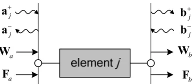
This section discusses the reflection and transmission matrices derived by the transfer matrix method. Figure 2.7 represents a linear element with input and output. For a linear mechanical system, it can be a combination of many linear subsystems, such as masses, springs, dampers, or linear continuous systems, such as bars, beams, plates and so on. Assuming that F and W are the internal force and displacement vectors with subscripts ‘a’ and ‘b’ indicating the input and output positions, they can be related by

11 12

21 22

a b

⎧ ⎫ ⎡ ⎤⎧ ⎫ =

⎨ ⎬ ⎢ ⎥⎨ ⎬

⎣ ⎦

⎩ ⎭ ⎩ ⎭

W Ω Ω W

F Ω Ω F (2.35)

(42)

is limited for some systems, in which cases, the internal force and displacement vectors can be related by other methods, such as the spectral element method [2]. All the systems discussed in this thesis can be analysed by the transfer matrix method.

[image:42.595.230.424.155.239.2]

a W a F b W b F j + a j − a j + b j − b

Figure 2.7 Element j with input and output forces and displacements.

If the element is a discontinuity connecting two waveguides a and b as shown in Figure 2.5, referring to equation (2.24), the displacements and internal forces on both sides can be related to waves amplitudes by

a ja ja j

+ − + + − − ⎡ ⎤ ⎧ ⎫ ⎧ ⎫_{= ⎢} ⎪ ⎪ ⎥ ⎨ ⎬ ⎨ ⎬ ⎢ ⎥ ⎪ ⎪ ⎩ ⎭ ⎣ ⎦ ⎩ ⎭

W Ψ Ψ a

F Φ Φ a and

b jb jb j

+ − + + − − ⎡ ⎤ ⎧ ⎫ ⎧ ⎫_{= ⎢} ⎪ ⎪ ⎥ ⎨ ⎬ ⎨ ⎬ ⎢ ⎥ ⎪ ⎪ ⎩ ⎭ ⎣ ⎦ ⎩ ⎭

W Ψ Ψ b

F Φ Φ b . (2.36)

Substituting equation (2.36) into (2.35) and rearranging, after some lengthy manipulation, yield

11 12 11 12

21 22 21 22

ja jb jb j ja jb jb j

− + + − + − − + − + + + + − − − ⎡ − − ⎤ ⎧ ⎫ ⎡_{⎪ ⎪} − + ⎤ ⎧ ⎫_{⎪ ⎪} = ⎢ ₋ ₋ ⎥⎨ ⎬ ⎢₋ ₊ ⎥⎨ ⎬ ⎢ ⎥⎪ ⎪ ⎢ ⎥⎪ ⎪ ⎣ ⎦ ⎩ ⎭ ⎣ ⎦ ⎩ ⎭

Ψ Ω Ψ Ω Φ a Ψ Ω Ψ Ω Φ a

Φ Ω Ψ Ω Φ b Φ Ω Ψ Ω Φ b . (2.37)

The following introduces the method to obtain the reflection and transmission coefficients.

Assuming that the matrix on the left-hand side is invertible, then

1

11 12 11 12

21 22 21 22

j ja jb jb ja jb jb j

− − − + + + − − + + − + + + − − − ⎧ ⎫ ⎡ − − ⎤ ⎡− + ⎤ ⎧ ⎫ ⎪ ⎪_{= ⎢} ⎪ ⎪ ⎥ ⎢ ⎥ ⎨ ⎬ ₋ ₋ ₋ ₊ ⎨ ⎬ ⎢ ⎥ ⎢ ⎥ ⎪ ⎪ ⎪ ⎪ ⎩ ⎭ ⎣ ⎦ ⎣ ⎦ ⎩ ⎭

a Ψ Ω Ψ Ω Φ Ψ Ω Ψ Ω Φ a

b Φ Ω Ψ Ω Φ Φ Ω Ψ Ω Φ b . (2.38)

The first matrix on the right-hand side can be written as

11 12 11 12

21 22 21 22

ja jb jb

− + + − + + ⎡ − − ⎤ ⎡ ⎤ = ⎢ ₋ ₋ ⎥ ⎢ ⎥ ⎢ ⎥ ⎣ ⎦ ⎣ ⎦

Ψ Ω Ψ Ω Φ B B

Φ Ω Ψ Ω Φ B B . (2.39)

By using the partitioned inverse, it can be obtained that

1

11 12 11 12

21 22 21 22

−

⎡ ⎤ ⎡ ⎤

=

⎢ ⎥ ⎢ ⎥

⎣ ⎦ ⎣ ⎦

C C B B

C C B B (2.40)

(43)

(

₁

)

1

11 11 12 22 21

1

12 11 12 22

1

21 22 21 11

1 1 1

22 22 22 21 11 12 22

, , , . − − − − − − − = − = − = − = +

C B B B B

C C B B

C B B C

C B B B C B B

(2.41)

Substituting equation (2.40) into (2.38) and comparing the result with equation (2.29), the reflection and transmission matrices are given by

(

)

(

)

(

)

(

)

11 12

11 11 12 12 21 22

21 22

21 11 12 22 21 22

,

, ,

.

aa

j ja ja

ba

j jb jb jb jb

ab

j ja ja

bb

j jb jb jb jb

+ + − − − − + + − − − − = − − = + + + = − − = + + +

R C Ψ C Φ

T C Ω Ψ Ω Φ C Ω Ψ Ω Φ

T C Ψ C Φ

R C Ω Ψ Ω Φ C Ω Ψ Ω Φ

(2.42)

The reflection matrix can also be obtained for a boundary by setting the terms with subscript b to zero.

Some techniques can be used to simplify the process when only reflection and transmission coefficients of a particular wave mode are of interest. Substituting equation (2.29) into (2.37) and rearranging gives

11 12 11 12

21 22 21 22

aa ba

ja jb jb j j ja jb jb j

ab bb

ja jb jb j j ja jb jb j

− + + + − − + − + + + − − − ⎧⎡ − − ⎤ ⎡ ⎤ ⎡− + ⎤ ⎧ ⎫⎫ ⎪ ₋ ⎪⎪ ⎪₌ ⎢ ⎥ ⎢ ⎥ ⎢ ⎥ ⎨ ₋ ₋ ₋ ₊ ⎬⎨ ⎬ ⎢ ⎥ ⎢ ⎥ ⎢ ⎥ ⎪ ⎪ ⎪⎣ ⎦ ⎣ ⎦ ⎣ ⎦ ⎩ ⎭⎪ ⎩ ⎭

Ψ Ω Ψ Ω Φ R T Ψ Ω Ψ Ω Φ a

0

Φ Ω Ψ Ω Φ T R Φ Ω Ψ Ω Φ b . (2.43)

When only one wave mode is assumed to exist in a+_j, by substituting a+_j and b−_j =0 into the above equation, the corresponding reflection and transmission coefficients can be determined easily from the above equation. The next section discusses such an example. This method can also be used to obtain the reflection at boundaries.

Joint identification in structural waveguides using wave reflection and transmission coefficients

University of Southampton Research Repository

ePrints Soton

FACULTY OF ENGINEERING, SCIENCE AND MATHEMATICS

INSTITUTE OF SOUND AND VIBRATION RESEARCH

Joint Identification in Structural Waveguides

Using Wave Reflection and Transmission

Coefficients

A thesis submitted for the degree of

Doctor of Philosophy

Abstract

Faculty of Engineering, Science and Mathematics

Institute of Sound and Vibration Research

Doctor of Philosophy

Joint Identification in Structural Waveguides Using Wave

Reflection and Transmission Coefficients

Acknowledgements

Declaration of Authorship

Table of Contents

List of Figures

List of Tables

(

)

Glossary of Symbols

[ ]

[ ]

{ }

(

)

Chapter 1 Introduction

1.1 Background

1.2 Modelling Methodologies

1.3 Wave Propagation Approach

1.4 Uncertainties of Joints and Discontinuities

1.5 Brief Introduction to Joint Identification

1.6 Objectives

1.7 Contributions of the Thesis

1.8 Overview of the Thesis

Chapter 2 Wave Propagation, Reflection and

Transmission in Waveguides

2.1 Introduction

2.2 Longitudinal Wave Propagation in Rods

2.3 Flexural Wave Propagation in Beams

( )

( )

2.4 Damping Effects of Waveguides

(

)

(

)

(

)

2.5 Reflection and Transmission coefficients

2.6 A General Wave Approach

2.7 Reflection and Transmission Coefficients in Terms of

Parameters of Discontinuities

(

)

(

)

(

) (

)

(

) (

)

(

)

(

)

(

)

(

)

(

)

2.8 Case Study: Reflection and Transmission Coefficients of

Two Identical Semi-infinite Beams Connected by a

Discontinuity