Algorithms for deterministic balanced subspace identification

www.elsevier.com/locate/automatica

Algorithms for deterministic balanced subspace identification

夡

Ivan Markovsky

, Jan C. Willems

, Paolo Rapisarda

, Bart L.M. De Moor

a_{ESAT, SCD-SISTA, K.U.Leuven, Kasteelpark Arenberg 10, B-3001 Leuven-Heverlee, Belgium} b_{Department of Mathematics, University of Maastricht, 6200 MD Maastricht, The Netherlands}

Received 22 January 2004; received in revised form 7 October 2004; accepted 21 October 2004 Available online 13 January 2005

Abstract

New algorithms for identification of a balanced state space representation are proposed. They are based on a procedure for the estimation of impulse response and sequential zero input responses directly from data. The proposed algorithms are more efficient than the existing alternatives that compute the whole Hankel matrix of Markov parameters. It is shown that the computations can be performed on Hankel matrices of the input–output data of various dimensions. By choosing wider matrices, we need persistency of excitation of smaller order. Moreover, this leads to computational savings and improved statistical accuracy when the data is noisy. Using a finite amount of input–output data, the existing algorithms compute finite time balanced representation and the identified models have a lower bound on the distance to an exact balanced representation. The proposed algorithm can approximate arbitrarily closely an exact balanced representation. Moreover, the finite time balancing parameter can be selected automatically by monitoring the decay of the impulse response. We show what is the optimal in terms of minimal identifiability condition partition of the data into “past” and “future”.

䉷2004 Elsevier Ltd. All rights reserved.

Keywords: Exact deterministic subspace identification; Balanced model reduction; Approximate system identification; MPUM

1. Introduction

In this paper, we consider the following exact determinis-tic identification problem: given an input–output trajectory

˜

w=(u,˜ y)˜ ,w˜ =(w˜(1), . . . ,w˜(T )), of an LTI system

S: x(t_y(t)+1₌)_Cx(t)=Ax(t)_+Du(t),+Bu(t) (1)

u(t) ∈ Rm, y(t) ∈ Rp, x(t) ∈ Rn, determine fromw an˜

associated balanced state model (Moore, 1981; Pernebo & Silverman, 1982)

Sbal: xbal(t_y(t)+₌1)_Cbalxbal(t)=Abalxbal(t)_+Dbalu(t).+Bbalu(t)

夡_{This paper was not presented at any IFAC meeting. This paper was} recommended for publication in revised form by Associate Editor B. Ninness under the direction of Editor T. Soderstrom.

∗_{Corresponding author. Fax: +32-16-321970.}

E-mail addresses:[email protected] (I. Markovsky),[email protected](J.C. Willems), [email protected](P. Rapisarda),

[email protected](B.L.M. De Moor).

0005-1098/$ - see front matter䉷2004 Elsevier Ltd. All rights reserved. doi:10.1016/j.automatica.2004.10.007

The given trajectoryw˜ =(u,˜ y)˜ is an exact trajectory ofS. This means that there exists x(˜ 1) ∈ Rn, such that the re-sponse of Sto the inputu˜ and initial conditionx(˜ 1)isy˜. The problem is to find conditions and algorithms to con-struct Sbal directly fromw. Although the assumption that˜

˜

w is exact is mainly of theoretical importance, we believe

that solving the exact identification problem is a prerequi-site for the study of the realistic approximate identification problems.

to find an input/state/output balanced representation of the

most powerful unfalsified model (MPUM).

The balanced state-space identification problem is stud-ied inMoonen and Ramos (1993)andVan Overschee and De Moor (1996, Chapter 5). The proposed algorithms fit in the outline given below, which will be called the ba-sic algorithm. The following notation is used: with f =

(f (1), . . . , f (T )), H_(f ):=

    

f (1) f (2) f (3) · · · f (T −+1) f (2) f (3) f (4) · · · f (T −+2) f (3) f (4) f (5) · · · f (T −+3)

... ... ... ...

f () f (+1) f (+2) · · · f (T )      

and is the shift operator f (t) := f (t +1). Acting on a vector or matrix, removes the first block-row. By f we will denote both the time series (f (1), . . . , f (T ))and the vector col(f (1), . . . , f (T )), where col(·)denotes a (block) column vector.

Algorithm 1 (Basic algorithm). Input: a time series w˜ =

(u,˜ y)˜ , an upper boundnmaxof the system order, and a finite time balancing parameter>nmax.

1. Find the first 2 samples H(0), . . . , H (2−1) of the impulse response matrix of S and let H := col(H(0), . . . , H (2−1)).

2. Find zero input responsesy₀(1), . . . , y₀(M), M := T −

+1, of length , generated from initial conditions x(1)

0 , . . . , x0(M) that form a valid state sequence of S obtained by the inputu˜. LetY0:= [y₀(1) · · · y₀(M)]. 3. Compute the restricted SVD,H=UV, of the block

Hankel matrix of Markov parametersH=H(H )∈ Rp×m.

4. Compute the balanced state sequence Xbal˜ :=

−1_UY0,

˜

Xbal= [ ˜xbal(nmax+1) · · · xbal(˜ nmax+M)]. 5. Compute the finite time balanced realization Abal,

Bbal,Cbal,Dbalby solving the linear system of equations

˜

xbal(nmax+2)) · · · xbal(˜ nmax+M)

˜

y(nmax+1) · · · ˜y(nmax+T −)

=

Abal Bbal Cbal Dbal

×

˜

xbal(nmax+1) · · · ˜xbal(nmax+T −)

˜

u(nmax+1) · · · u(˜ nmax+T −) . (2)

Output: a finite time- balanced representation (Abal, Bbal,Cbal,Dbal) ofS.

Note 1 (Finite time-balancing). The basic algorithm

fac-tors a finite×block Hankel matrix of Markov parame-tersH, so that the obtained representation (Abal,Bbal,Cbal,

Dbal) is finite time- balanced. For nmax, the repre-sentation obtained is close to an infinite time balanced one. Determining an appropriate value for the parameter, how-ever, is a problem in its own right, and will be addressed in the paper.

Note 2 (Model reduction). Identification of a state-space model in a balanced basis is motivated by the effective heuristic for model reduction by truncation in that basis. In principle, it is possible to identify the model in any basis and then apply standard algorithms for state transformation to a balanced basis. The direct algorithm discussed in this paper, however, has the advantage over the indirect approach that it allows to identify a reduced order model directly from data without ever computing a full order model.

The model reduction can be done by Step 5 of the basic algorithm. Let r be the desired order of the reduced model and letXred˜ be the truncated to the first r rows balanced state sequenceXbal˜ . As a heuristic model reduction procedure, we derive the reduced model parameters by solving the

least-squares problem

˜

xred(nmax+2) · · · xred(˜ nmax+M)

˜

y(nmax+1) · · · ˜y(nmax+T −)

=

Ared Bred Cred Dred

×

˜

xred(nmax+1) · · · ˜xred(nmax+T −)

˜

u(nmax+1) · · · u(˜ nmax+T −)

in place of the exact system of equations (2). The obtained model(Ared, Bred, Cred, Dred)is not the same as the model obtained by truncation of the (finite time-) balanced model. In particular, we do not know about error bounds similar to the ones available for the (infinite time) balanced model reduction. The model reduction question is not further dis-cussed in this paper and will be treated elsewhere.

Note 3. InMoonen and Ramos (1993);Van Overschee and

De Moor (1996), it is not mentioned that the Hankel ma-trix of Markov parametersHis computed. Also inMoonen and Ramos (1993), it is not mentioned that the matrixY0of sequential zero input responses is computed. In the present paper, we interpret these algorithms as implementations of the above basic algorithm and reveal their structure. The im-portant difference among the algorithms of Moonen–Ramos, Van Overschee–De Moor, and Algorithm 7 proposed in this paper is namely the method of computation of the matrixY0 and the impulse response H.

Algorithm 2. Input: a time seriesw˜=(u,˜ y)˜ , an upper bound

nmaxof the system order, and a finite time balancing param-eter>nmax.

1. Find the first 2 samples H(0), . . . , H (2−1) of the impulse response matrix of S and let H := col(H(0), . . . , H (2−1)).

2. Compute the restricted SVD,H=UV, of the block Hankel matrix of Markov parametersH=H(H )∈ Rp×m.

3. DefineObal:=U

√

andCbal:=

√ V_.

4. LetDbal=H (0),Bbalbe equal to the firstmcolumns of

Cbal (the first block column),Cbal be equal to the first

p rows of Obal (the first block row), and Abal be the solution of the equation(∗Obal)Abal=Obal, where and∗, acting on a block matrix, remove, respectively, the first and the last block rows.

Output: a finite time- balanced representation (Abal, Bbal,Cbal,Dbal) ofS.

In Algorithm 2, once the impulse response is computed, the parametersAbal,Bbal, Cbal,Dbal are obtained without returning to the original observed data. Yet another alterna-tive for computing a balanced representation directly from data is to obtain the parameters Abal andCbal as in Algo-rithm 2 fromObaland the parametersBbalandDbal(as well as the initial conditionxbal(1), under whichw is obtained)˜

from the linear system of equations

˜

y(t)=CbalAtbalxbal(1)+

t−1

=1

CbalAt−1−

bal Bbalu(˜ )

+Dbal(t+1), fort=1, . . . , T, (3) using the original data. (By using Kronecker products (3) can be solved explicitly.) The resulting Algorithm 3 is in the spirit of the MOESP-type algorithms, seeVerhaegen and Dewilde (1992).

Algorithm 3. Input: a time seriesw˜=(u,˜ y)˜ , an upper bound nmaxof the system order, and a finite time balancing param-eter>nmax.

1. Find the first 2 samples H(0), . . . , H (2−1) of the impulse response matrix of S and let H := col(H(0), . . . , H (2−1)).

2. Compute the restricted SVD,H=UV, of the block Hankel matrix of Markov parametersH=H(H )∈ Rp×m.

3. DefineObal:=U

√ .

4. LetCbal be equal to the first p rows ofObal (the first block row), andAbalbe the solution of the equation

(∗Obal)Abal=Obal.

5. Solve (3) forBbal,Dbal, andxbal(1).

Output: a finite time- balanced representation (Abal, Bbal,Cbal,Dbal) ofS.

Simulation results show that in the presence of noise “go-ing back to the data”, as done in the basic algorithm and in Algorithm 3, leads to more accurate results. This gives an indication that the basic algorithm and Algorithms 3 might be superior to Algorithm 2 in the noisy case.

The outline of the paper is as follows. In Section 2 we present two lemmas that are instrumental for the derivation of the algorithm. The first one, which we call the

fundamen-tal lemma, gives conditions on a trajectoryw, under which˜

any response of S with length L belongs to the image of the Hankel matrixHL(w˜). As a consequence, any response of length L can be found as HL(w˜)g for a suitable g ∈ RT−L+1_{. The second lemma, which we call the weaving}

lemma, shows how an arbitrary long response of Scan be obtained from a finite amount of dataw by weaving together˜

segments of the desired response.

In Section 3, the fundamental lemma is applied for con-struction of the impulse response H. Theorem 4 gives an algorithm for the computation of H, based on the construc-tionH=H2(w˜)G, for a suitable G. This approach gives a limited length response. Using the weaving lemma, an al-gorithm is derived that computes arbitrary many samples of the impulse response. By monitoring the decay of the im-pulse response while computing it, the parameter of the basic algorithm can be chosen adaptively.

In Section 4, an algorithm for the computation of the matrix Y0 that appears in the basic algorithm is described. It is also based on the fundamental lemma and in anal-ogy with the impulse response computation has a block version and an iterative version. We show that the block version of the algorithm is actually equivalent to the fa-mous oblique projection from the classical subspace algo-rithms, which gives a system theoretic interpretation of the oblique projection. (In the subspace identification literature the oblique projection is defined and interpreted as a geo-metric operation and its system theoretic meaning remains hidden.)

2. Fundamental lemmas

Denote byB|_[1,L]the set of all trajectories of the system

Sover the time interval[1, L], i.e.,

B|[1,L]:=

w=

u y :=

u(1) y(1) , . . . ,

u(L) y(L)

∃x(1), . . . , x(L+1)such that(1)holds}.

The notion of persistency of excitation is defined next, cf. (Van Overschee & De Moor, 1996, Definition 5).

Definition 1 (Persistency of excitation). The sequenceu˜=

Lemma 2 (Fundamental lemma Willems, Rapisarda, Markovsky, and DeMoor (2004)). Let

1. w˜ =(u,˜ y)˜ be a trajectory of the LTI systemS, i.e.,

˜

w=

˜

u

˜

y =

˜

u(1)

˜

y(1) , . . . ,

˜

u(T )

˜

y(T ) ∈B|[1,T]; 2. the systemSbe controllable; and

3. the input sequence u˜ be persistently exciting of order

L+n, wherenis the order (the dimension of the state space) ofS.

Then any L samples long trajectory w=(u, y)ofScan be written as a linear combination of the columns ofHL(w˜) and any linear combinationHL(w˜)g,g∈RT−L+1, is also

a trajectory ofS, i.e., col span(HL(w˜))=B|_[1,L]. Proof. The proof of these results as well as interesting corol-laries are given inWillems et al. (2004).

The fundamental lemma states conditions under which the Hankel matrixHL(w˜)has the “correct” image (and as a consequence the “correct” left kernel). The conditions are not verifiable from the dataw alone, so that in identification˜ problems, where onlyw is given, they should be assumed.˜ In addition, for the derivation of the algorithm, we assume that an upper boundnmaxon the system ordernand an up-per bound lmax on the system lag l are a priori known. The system lagl is defined as the observability index of

S. Note that nmaxcan be used as a loose upper bound on

l. Genericallypl=nandplmax=nmax. Assumptions 1–3

of the fundamental lemma and the assumption thatnmax is given are the standard assumptions for deterministic sub-space identification, see, e.g.,Van Overschee and De Moor (1996, Chapter 2).

The next lemma shows how a long response can be con-structed by weaving together short ones.

Lemma 3 (Weaving responses). Let

1. w˜(1) be aT1 samples long trajectory ofS, i.e.,w˜(1)∈

B|[1,T1];

2. w˜(2) be aT2 samples long trajectory ofS, i.e., w˜(2)∈

B|[1,T2];

3. the last l samples ofw˜(1)coincide with the first l samples ofw˜(2), i.e.,

(w˜(1)(T1−l+1), . . . ,w˜(1)(T1))

=(w˜(2)(1), . . . ,w˜(2)(l));

4. l is larger than or equal to the laglof the systemS.

Then the trajectory

w:=(w˜(1)(1), . . .,w˜(1)(T1),w˜(2)(l+1), . . .,w˜(2)(T2)), (4)

obtained by weaving togetherw˜(1) and w˜(2) is a trajectory ofS, i.e., w∈B|_[1,T1+T2−l].

Proof. Let x˜(1) :=(x˜(1)(1), . . . ,x˜(1)(T1+1)) andx˜(2) :=

(x˜(2)_{(1), . . . ,x˜}(2)_{(T2+1))be the state sequences ofS} as-sociated with w(1)and w(2), respectively. Assumptions 3 and 4 imply thatx˜(1)(T1+1)= ˜x(2)(l+1). Therefore, (4) is a trajectory ofS.

3. Computation of the impulse response

In this section, we consider Step 1 of the basic algorithm: given a trajectoryw˜=(u,˜ y)˜ , find the first 2samples H of the impulse response ofS. We need the first 2samples of the impulse response in order to construct the×block Hankel matrixH(H ), whose factorization in turn gives the finite time-balancing transformation.

From the fundamental lemma, we know that, under suit-able conditions, col span(H2(w˜))=B|[1,2]. This implies that there exists a matrix G, such thatH2(y)G˜ =H. Thus, the problem reduces to the one of finding a particular G.

Let row dim denote the number of block rows of a matrix or vector and defineUp,U_f,Yp,Y_{f as follows}

Hlmax+2(u)˜ =:

Up

U_f , Hlmax+2(y)˜ =:

Yp Y_f ,

where row dim(Up) = row dim(Yp) = lmax and row dim(_Uf)=row dim(_Yf)=2.

Theorem 4 (Impulse response from data). Let w˜ =(u,˜ y)˜

be a trajectory of a controllable LTI system S of order

nnmaxand lagllmaxand letu˜be persistently exciting

of order 2+lmax+nmax. Then the system of equations

_Up

U_f Yp

G=

  

0_ml max×m

Im 0_m(2−1)×m

0_pl max×m

 

, (5)

is solvable for G ∈ R•×m. Moreover, for any particular

solutionG¯, the matrixY_fG¯ contains the first 2samples of the impulse response ofS, i.e.,Y_fG¯ =H.

Proof. Under the assumptions of the theorem, we can apply the fundamental lemma withL=lmax+2, thus

col span(Hl

max+2(w˜))=B|[1,lmax+2].

First we show that (5) is solvable. The impulse response

Im

0_m(2−1)×m , H

is a (matrix valued) response of S

obtained under zero initial conditions. Because of the zero

initial conditions,

Im

0_m(2−1)×m , H

preceded by any

exists a matrixG¯, such that    Up Uf Yp Y_f   G¯ =

    

0_ml max×m

Im 0_m(2−1)×m

0_plmax×m H     .

This shows that there exists a solutionG¯ of (5) and therefore YfG¯ is the impulse response.

Conversely, let G be a solution of (5). We have

   Up Uf Yp Y_f  

G=

    

0_ml max×m

Im 0_m(2−1)×m

0_plmax×m YfG

   

 (6)

and the fundamental lemma guarantees that the right-hand side of (6) is a response ofS. The response is identically zero during the firstlmaxsamples, which (using the assump-tionlmaxl) guarantees that the initial conditions are set to zero. The input

Im 0_m(2−1)×m

is a matrix valued impulse,

so that the corresponding outputY_fGis indeed the impulse response H.

Theorem 1 gives the following block algorithm for the computation of H.

Algorithm 4 (Block computation of the impulse re-sponse). Input:u˜,y˜,lmax, and.

1. Solve the system of Eq. (5). Let G¯ be the computed solution.

2. ComputeH=Y_fG¯.

Output: the first 2samples of the impulse response H.

Note 4 (Efficient implementation via QR factorization). The system of equations in Step 1 of Algorithm 4 can be solved efficiently by first “compressing the data” via the QR de-composition

U U

⊥

⊥ ⊥ ⊥ ⊥

f Yp

p | Yf = QR , R =:

R11 0 R21 R22

,

[

[

[

[

whereR11 ∈ R(m(lmax+2)+plmax)×(m(lmax+2)+plmax)_{, and} then computing the pseudo-inverse of the R11 block. We have

H=Yf

_Up

Uf Yp

+₀

I 0

=R21R11+ ₀

I 0

.

We proceed to point at an inherent limitation of Algorithm 4 when dealing with finite amount of data.

Let T samples of the input and the output be given. The persistency of excitation assumption in Theorem 4 requires that H_2+lmax+nmax(u)˜ is full row rank, which

implies that

m(2+lmax+nmax)T −(2+lmax+nmax)+1

⇒1

2

T +1

m+1 −lmax−nmax

.

Thus using Algorithm 4, we are limited in the number of samples of the impulse response that can be computed. Moreover, for efficiency and accuracy (in the presence of noise), we want to have Hankel matricesUp,U_{f, etc., with} many more columns than rows, which implies small.

According to Lemma 3, however, it is possible to find arbitrary many samples of the impulse response. Algorithm 5 does this by computing iteratively blocks of L consecutive samples, where

1L1 2

_{T +}

1

m+1 −lmax−nmax

. (7)

Moreover, monitoring the decay of H (provided the system is stable) while computing it, gives a heuristic way to determine the parameter.

In the recursive algorithm the matrices Up, U_f, Yp, Y_f defined above are redefined as follows:

Hlmax+L(u)˜ =:

Up

U_f , Hlmax+L(y)˜ =:

Yp Y_f ,

where row dim(Up)=row dim(Yp)=lmax and row dim (Uf)=row dim(Yf)=L.

Algorithm 5 (Iterative computation of the impulse

re-sponse). Input:u˜,y˜,nmax,lmax, and eitheror a conver-gence toleranceε.

1. Choose the number of samples L computed in one iter-ation step according to the persistency of excititer-ation of

˜

u. In particular (7) should be satisfied.

2. Initialization: k := 0, Fu(0) :=

₀

mlmax×m

Im 0_m(L−1)×m

and

F(0)

y,p:=0plmax. 3. Repeat

3.1. Solve the system

_Up

Uf Yp

G(k)₌Fu(k) Fy(k),p

.

3.2. Compute the responseH(k):=F(k)

y,f :=YfG(k). 3.3. DefineFy(k):=

Fy(k),p F_y(k)_,f

.

3.4. ShiftFu andFy: Fu(k+1) :=

L_F(k)

u 0_mL×m ,F

(k+1) y,p :=

L_F(k)

y .

3.5. Increment the iteration counterk:=k+1.

4. Until

kL2 ifis given,

H(k−1)

Output:H=col(H(0), . . . , H(k−1))andifis not given as an input.

Proposition 5. Let(u,˜ y)˜ be a trajectory of a controllable

LTI systemSof order nnmaxand lagllmax, and let

˜

ube persistently exciting of orderL+lmax+nmax. Then

Algorithm 5 computes the first 2 samples of the impulse response ofS.

Proof. Under the assumptions of the proposition, we can applyTheorem 1, with the parameterin the theorem, re-placed by the parameter L, selected on Step 1 of the algo-rithm. Steps 3.1 and 3.1 of the recursive algorithm corre-spond to the steps of the block algorithm. The right-hand

side

Fu(k)

Fy(k),p of the system of equations, solved in Step 3.1, is initialized so thatH(0) is indeed the matrix of the first L samples of the impulse response.

The response computed on the(k+1)th iteration step,

k1, is a response due to zero input and its firstlmax sam-ples overlap the lastlmaxsamples of the response computed on the kth iteration step. By the weaving lemma, their con-catenation is a valid response. Applying this argument re-cursively, we have that H computed by the algorithm is the impulse response of the system.

Note 5 (Computation of an arbitrary response from data). For the purpose of balanced subspace identification, we need construction of the impulse response from data. In Markovsky, Willems, Rapisarda, and De Moor (2004), Theorem 4 and Algorithm 5 are modified to compute an arbitrary response directly from data.

Note 6 (Efficient implementation via QR factorization). The most expensive part of Algorithm 4 is solving the system of equations on Step 3.1. It can be solved efficiently via the QR factorization as described in Note 4. Moreover, since the matrix on the left-hand side of the system is fixed, the pseudo-inverse can be computed out of the iteration loop and used for all iterations.

4. Computation of sequential zero input responses

In this section, we consider step 2 of the basic algorithm: givenw˜ =(u,˜ y)˜ , find a sequential zero input responsesY0 ofS. By “sequential”, we mean that the initial conditions corresponding to the columns ofY0 form a valid state se-quence ofS.

Using the fundamental lemma, a set of zero input trajec-tories can be computed from data by solving the system of equations

_Up

Uf Yp

G=

_Up

0 Yp

(8)

and settingY0=Y_fG. Moreover, the Hankel structure ofUp and Yp imply that Y0 is a matrix of sequential responses. System (8) and Y0=Y_fG give a block algorithm for the computation of sequential zero input responses. It is analo-gous to the block algorithm for the computation of the im-pulse response and again the computation can be performed efficiently via the QR factorization.

Note 7 (Connection with the oblique projection). For any particular solutionG¯ of (8),Y0=Y_fG¯ is equal to the oblique

projectionY_f/_U

fWp,Wp:=

Up

Yp of the classical subspace algorithms. To show this, let

¯

G= [W p U_f]

_WpW

p WpU_f U_fW

p UfU_f

+_Wp

0

be the least-squares least norm solution of

_Up

Yp Uf

G=

_Up

Yp 0

,which is (8) with permuted rows, so that the

solu-tion is not changed. Then

YfG¯ =Yf[Wp U_f]

_WpW

p WpU_f UfWp UfU_f

+_Wp

0 , (9)

which is the definition of the oblique projection Y_f/_U fWp, see Van Overschee and De Moor (1996, p. 21, Eq. (1.4). Thus, the oblique projection is an implementation of the block algorithm for the computation of the sequential zero input responsesY0.

We proceed to present a recursive algorithm for the com-putation of Y0, analogous to Algorithm 5 for the computa-tion of the impulse response. An advantage of the recursive algorithm over the block one is that one is not restricted by the finite amount of dataw to a finite length responses˜ Y0.

Algorithm 6 (Sequential zero input responses). Input: u, y, nmax,lmax, and either the desired number of samplesor a convergence toleranceε.

1. Choose the number of samples L computed in one iter-ation step according to the persistency of excititer-ation of

˜

u. In particular (7) should be satisfied. 2. Initialization:k:=0,Fu(0):=

Up

0 , andF

(0) y,p:=Yp. 3. Repeat

3.1. Solve the system

_Up

U_f Yp

G(k)₌Fu(k) Fy(k),p

.

3.2. Compute the responseY₀(k):=F(k)

y,f :=YfG(k). 3.3. DefineFy(k):=

Fy(k),p F_y(k)_,f

3.4. Shift Fu and Fy: Fu(k+1) :=

L_F(k)

u

0_mL×m , and F(k+1)

y,p :=LFy(k).

3.5. Increment the iteration counterk:=k+1.

4. Until

kL ifis given,

Y(k−1)

0 Fε otherwise.

5. Ifis not given as an input, define:=kL.

Output:Y0=col(Y₀(0), . . . , Y₀(k−1))and, ifis not given as an input.

Proposition 6. Under the assumptions of Proposition 5,

Algorithm 6 computes a matrix of sequential zero input re-sponses ofSwithblock rows.

Proof. Similar to the proof of Proposition 5.

Note 8 (Efficient implementation via QR

factoriza-tion). Note 6is valid also for Algorithm 6. Moreover, in the

basic algorithm, where both Algorithms 5 and 6 are applied, the pseudo-inverse needs to be computed only once.

5. An algorithm for deterministic balanced subspace identification

In the previous sections, we have specified Steps 1 and 2 of the basic algorithm. Steps 3–5 follow from standard derivations, which we now repeat for completeness. Let H be the Hankel matrix of the Markov parameters H :=

H(H ). By factoring H into Obal and Cbal via the

re-stricted SVD

H=UV=U √ Obal

√

V

Cbal

, ∈Rn×n

we obtain an extended observability matrix

Obal=col(Cbal, CbalAbal, . . . , CbalA_bal−1)

and a corresponding extended controllability matrix

Cbal= [Bbal AbalBbal · · · A_bal−1Bbal]

in a finite time balanced basis. The basis is finite time- balanced, because the finite time- observability gramian

O

balObal=and the finite time-controllability gramian

CbalCbal=are equal.

The matrix of sequential zero input responsesY0 can be written asY0=OXfor a certain extended observability ma-trixOand a state sequence X in the same basis. We find the balanced state sequence

˜

Xbal:= [ ˜xbal(lmax+1) · · · xbal(˜ lmax+T +1−L)] corresponding toObal=U

√ from

Y0=ObalXbal˜ ⇒ ˜Xbal=

−1_UY0.

The corresponding balanced representation (Abal, Bbal, Cbal, Dbal) is computed from the system of equations

˜

xbal(lmax+2)2) · · · ˜xbal(lmax+T +1−L)

˜

y(lmax+1) · · · y(˜ lmax+T −L)

=

Abal Bbal Cbal Dbal

×

˜

xbal(lmax+1) · · · ˜xbal(lmax+T −L)

˜

u(lmax+1) · · · u(˜ lmax+T −L) . (10)

This yields the following procedure.

Algorithm 7. Input:u˜,y˜,nmax,lmax, and either>nmax

or a convergence toleranceε.

1. Apply Algorithm 5 with inputs u˜, y˜, nmax, lmax, and eitherorε, in order to compute the impulse response

H and, if not given, the parameter. In the latter case, let:=max(nmax+1,)

2. Apply Algorithm 6 with inputs u˜, y˜, nmax, lmax, L, and , in order to compute the sequential zero input responsesY0.

3. Form the Hankel matrixH :=H(H )and compute the restricted SVDH=UV.

4. Compute a balanced state sequenceXbal˜ =

−1_UY0. 5. Compute a balanced representation by solving (10).

Output:Abal,Bbal,Cbal,Dbal, and, ifis not given as an input.

The discussion in this section and Propositions 5 and 6 prove the following main result.

Theorem 7. Under the assumptions of Proposition 5, (Abal, Bbal, Cbal, Dbal)computed by Algorithm 7 is a finite time-balanced representation ofS.

6. Alternative algorithms

We outline the algorithms of Van Overschee–De Moor and Moonen–Ramos.

Algorithm 8 (Van Overschee & De Moor, 1996). Input:u˜,

˜

y, and a parameter i. Define:

Up

Uf :=H2i(u)˜ , where row dim(Up)=i, and

Yp

Y_f :=H2i(˜y), where row dim(Yp)=i.

1. Compute the weight matrix W := U_p(UpU_p)−1J, where J is the left–right flipped identity matrix.

2. Compute the oblique projectionY0:=Y_f/_U f

Up Yp . 3. Compute the matrixHˆ :=Y0Wand the restricted SVD,

ˆ

4. Compute a balanced state sequenceXbal=−1UY0. 5. Compute a balanced representation by solving (10).

Output:Abal,Bbal,Cbal,Dbal.

Note 9. The weight matrix W is different from the one in Van Overschee & De Moor (1996). In terms of the final re-sultHˆ, however, it is equivalent. Another difference between Algorithm 8 and the deterministic balanced subspace algo-rithm ofVan Overschee & De Moor (1996)is that the shifted state sequence appearing on the left-hand side of (10) is re-computed inVan Overschee & De Moor (1996)by another oblique projection.

Algorithm 9 (Moonen & Ramos, 1993). Input:u˜,y˜, and a parameter i.

Define:

Up

Uf :=H2i(˜u), where row dim(Up)=i, and

Yp

Y_f :=H2i(y)˜ , where row dim(Yp)=i.

0. Compute a matrix [T1T2T3T4], whose rows form a

basis for the left kernel of   

Up Yp Uf Yf

  .

1. Compute the Hankel matrix of Markov parametersH= T4+(T2T4+T3−T1)J.

2. Compute a matrix of zero input responses Y0 =

T4+[T1T2]

Up Yp .

3. Compute the restricted SVD,H=UV.

4. Compute a balanced state sequenceXbal=

−1_UY0. 5. Compute a balanced representation by solving (10).

Output:Abal,Bbal,Cbal,Dbal.

Note 10. In the algorithms of Van Overschee–De Moor and Moonen–Ramos, the parameter i plays the row of the finite time balancing parameterfrom the previous sections. Note that i is given and the “past” and the “future” are taken with equal length i.

Both Algorithms 8 and 9 fit in the outline of the basic algorithm but Steps 1 and 2 are implemented in rather dif-ferent ways. As shown in Note 7, the oblique projection

Y_f/U_f

Up

Yp is a matrix of sequential zero input responses. The weight matrix W, in the algorithm of Van Overschee–De Moor, is constructed so thatHˆ =Y0W is an approximation of the Hankel matrix of Markov parametersH; it is the sum ofHand a matrix of zero input responses.

The most expensive computation in the algorithm of Moonen–Ramos is Step 0, the computation of the

an-nihilators [T1 · · · T4]. The matrix [T1T2]

Up Yp is a non-minimal state sequence (the shift-and-cut operator (Rapisarda & Willems, 1997)) and T₄+ is a corresponding

extended observability matrix. Thus T₄+[T1T2]

Up Yp is a matrix of sequential zero input responses. It turns out that (T2T₄+T3−T1)J is an extended controllability matrix (in the same basis), so that T₄+(T2T₄+T3−T1)J is the Hankel matrix of Markov parametersH.

A major difference between the proposed Algorithm 7, from one side, and the algorithms of Van Overschee–De Moor and Moonen–Ramos, on the other side, is that in Algo-rithm 7 the Hankel matrixHis not computed but constructed from the impulse response that parameterizes it. This is a big computational saving because recomputing the same el-ements ofHis avoided. In addition, in approximate identifi-cation, wherew is not a trajectory of˜ S, the matricesHˆ and Hcomputed by the algorithms of Van Overschee–De Moor and Moonen–Ramos are in general no longer Hankel, while the matrixHin Algorithm 7 is by construction Hankel.

7. On the splitting of the data into “past” and “future”

In the algorithms of Moonen–Ramos and Van Overschee–

De Moor the block-Hankel matrices

Up U_f and

Yp Y_f are split into “past” and “future” of an equal length. A natural question is why this is necessary and furthermore what is “optimal” according to certain relevant criteria partitionings. These questions are open for a long time, in particular in the context of the stochastic identification problem, see De Moor (2003).

In Sections 3 and 4 we showed that the past Up, Yp is used to assign the initial conditions and the future U_f, Y_f is used to compute the response. By weaving consecutive segments of the response, as done in Algorithms 5 and 6, the number of block rows in the future does not need to be equal to the required length of the response. Thus from the perspective of deterministic identification, the answer to the above question is:

row dim(Up) = row dim(Yp) = lmax, i.e., the given least upper bound on the system lag l, and row dim(_Uf)=row dim(_Yf) ∈ {1, . . . ,−lmax +

nmax}, whereis the order of persistency of excitation of the inputu˜.

As shown inWillems et al. (2004, Section 4, Comment 5)

˜

upersistently exciting of orderlmax+1+nmax (11) is a sharp sufficient condition for identifiability of the sys-temS. By using the iterative algorithms for computation of the impulse response and sequential free responses with pa-rameterL=1, Algorithms 2, 3, and 7 are applicable under the same assumption, so that the partitioning “past=lmax and future=1” is consistent with (11).

Proposition 8. Let(u,˜ y)˜ be a trajectory of a controllable LTI systemSof ordernnmaxand lagli, and letu˜ be

persistently exciting of order 2i+nmax. Then the

represen-tations computed by Algorithms 8 and 9 are equivalent to

S. Moreover, the representation computed by Algorithm 9

is in a finite time-i balanced basis.

Proposition 8 shows that Algorithms 8 and 9 are not par-simonious with respect to the available data: the systemS could be identifiable with algorithms Algorithms 2, 3, and 7 but not with Algorithms 8 and 9.

Note that the persistency of excitation required by Algo-rithms 8 and 9 is a function of the finite time balancing parameter. This implies that with a finite amount of data, Algorithms 8 and 9 are limited in the ability to identify a balanced representation. In fact,

i

T +1 2(max(m,p)+1)

.

In contrast, the persistency of excitation required by Algo-rithms 2, 3, and 7 depends only on the upper bounds on the system order and the lag and thus these algorithms can com-pute an infinite time balanced representation if (11) holds.

8. Simulations

In this section, we show some examples illustrate some advantages of the proposed algorithms. In all the experi-ments the systemSis minimal with transfer function

C(Iz−A)−1_B+D

=_(z0₋.89172(z−0.5193)(z+0.5595)

0.4314)(z+0.4987)(z+0.6154).

The input is a unit variance white noise and the data avail-able for identification is the corresponding trajectory w of˜

S, corrupted by independent white noises with standard de-viation s. Although, our main concern is the correct work of the algorithms for exact data, i.e., withs=0, by varying the noise variance s, we can investigate empirically the per-formance under noise. The simulation time is T =100. In all experiments the upper boundsnmaxandlmaxare taken equal to the system ordern=3 and the parameter L is taken equal to 3.

Consider first the estimation of the impulse response. Fig. 1 shows the exact impulse response H of S and the estimate Hˆ computed by Algorithm 5. With exact data,

||H− ˆH||F =10−15, so that up to the numerical precision the match is exact. The plots onFig. 1show the deteriora-tion of the estimates when the data is corrupted by noise.

Consider next the computation of the zero input response.

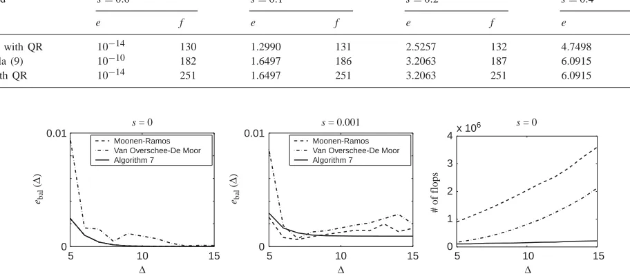
Table 1shows the error of estimatione:= ||Y0− ˆY0||F and the corresponding amount of operations, whereY0is a matrix of exact sequential zero input responses with length=10 andYˆ0is its estimate computed from data. The estimate is

computed in three ways: by Algorithm 6, implemented with the QR factorization, see Note 8; by the oblique projection, computed directly from (9); and by the oblique projection, computed via the QR factorization, see Note 7.

Algorithm 6 needs less computations and gives more ac-curate results than the alternatives. As already emphasized, the reason for this is that selecting the parameterL=nmax=3 instead ofL==10, as in a block computation, results in a more overdetermined system of equations in Step 3.1 of Algorithm 6 compared with system (8) used in the block al-gorithm. (For example, the difference is 95 vs. 88 columns.) As a result the noise is averaged over more samples, which leads to statistically better estimate. Solving several more overdetermined systems of equations instead of one more rectangular system can be more efficient, as it is in the exam-ple. In fact, the freedom in the choice of L makes it possible to optimize efficiency or another criterion.

All algorithms return a finite time balanced model. The next experiment illustrates the effect of the parameteron the balancing. LetWc/Wobe the controllability/observability gramians of an infinite time balanced model and Wcˆ /Woˆ be the controllability/observability gramians of an identified model. Define closeness to balancing by

e2 bal:=

||Wc− ˆWc||2

F + ||Wo− ˆWo||2F ||Wc||2

F + ||Wo||2F

.

Fig. 2 shows ebal as a function of for the three algo-rithms presented in the paper. The estimates obtained by Al-gorithm 7 and the alAl-gorithm of Moonen–Ramos are identi-cal estimate obtained by the algorithms of Van Overschee– De Moor is asymptotically equivalent, but for small , is worse. This is a consequence of the fact that this algorithm uses an approximation of the Hankel matrix of Markov pa-rameters.Fig. 2also showsebalas a function offor noisy data withs=0.001 and the total number of floating point operations (flops) required by the three algorithms.

9. Conclusions

The impulse response and the sequence of zero input re-sponses are the main tools for balanced subspace identifica-tion. Classically they are computed with the oblique projec-tion. We gave a system theoretic interpretation of the oblique projection and a new algorithm for computation of a re-sponse directly from data. The new algorithm allows compu-tation of an arbitrary long response from a finite data set and has the following advantages over the existing alternatives.

0 2 4 6 8 10 -1

-0.5 0 0.5 1

-1 -0.5 0 0.5 1

-1 -0.5 0 0.5 1 -1 -0.5 0 0.5 1

t s = 0.0

0 2 4 6 8 10

t s = 0.1

0 2 4 6 8 10

t s = 0.2

0 2 4 6 8 10

t s = 0.4

H(t), H(t)

ˆ

H(t), H(t)

ˆ

H(t), H(t)

ˆ

H(t), H(t)

ˆ

||H-H|| = 10ˆ -15 ||H-H|| = 0.02ˆ

||H-H|| = 0.21ˆ ||H-H|| = 0.05ˆ

Fig. 1. Impulse response estimation. Solid line—exact impulse response H, dashed line—impulse responseHˆ computed from data via Algorithm 5. Table 1

Error of estimatione= ||Y0− ˆY0||F and the corresponding amount of operations f in mega flops, whereY0is an exact sequence of zero input responses andY0ˆ is the estimate computed from data

Method s=0.0 s=0.1 s=0.2 s=0.4

e f e f e f e f

Alg. 6 with QR 10−14 130 1.2990 131 2.5257 132 4.7498 132

formula (9) 10−10 182 1.6497 186 3.2063 187 6.0915 189

(9) with QR 10−14 251 1.6497 251 3.2063 251 6.0915 252

5 10 15

0 0.01

Moonen-Ramos Van Overschee-De Moor Algorithm 7

∆

ebal

(

∆

)

ebal

(

∆

)

s = 0

5 10 15

0 0.01

Moonen-Ramos Van Overschee-De Moor Algorithm 7

∆

s = 0.001

5 10 15

0 1 2 3 4x 10

6

∆

# of flops

s = 0

Fig. 2. Closeness to balancingebaland computational cost as functions of the finite time balancing parameter.

of H many times. This is an inefficient step in these algorithms.

• In the algorithms of Moonen–Ramos and Van Overschee–De Moor, the parameteris supplied by the user. In the proposed algorithms, it can be determined automatically on the basis of a desired convergence

tolerance of the impulse response, which is directly related to the closeness of the obtained representation to a balanced one.

length of the given time seriesw. By choosing the pa-˜

rameterlarge enough, the proposed algorithms have no such limitation and can thus compute a representa-tion that is arbitrary close to an infinite time balanced one.

• The proposed algorithms have weaker persistency of excitation conditions than the one needed for the al-gorithms of Moonen–Ramos and Van Overschee–De Moor. As a result, in certain cases, the proposed algorithms are applicable, while the algorithms of Moonen–Ramos and Van Overschee–De Moor are not.

• In the proposed algorithms, the computations can be organized to use more overdetermined system of equa-tions, which result in more accurate estimates when w˜

is noisy.

We foresee other advantages on the level of the numer-ical implementation. Numernumer-ical issues, however, will be presented elsewhere.

Acknowledgements

Our research is supported by: Research Council KUL: GOA-Mefisto 666, several PhD/postdoc & fellow grants; Flemish Government: FWO: PhD/postdoc grants, projects, G.0240.99 (multilinear algebra), G.0407.02 (support vector machines), G.0197.02 (power islands), G.0141.03 (Identifi-cation and cryptography), G.0491.03 (control for intensive care glycemia), G.0120.03 (QIT), G.0800.01 (collective intelligence), research communities (ICCoS, ANMMM); AWI: Bil. Int. Collaboration Hungary/ Poland; IWT: PhD Grants, Soft4s (softsensors), Belgian Federal Government: DWTC (IUAP IV-02 (1996-2001) and IUAP V-22 (2002-2006), PODO-II (CP/40: TMS and Sustainability); EU: CAGE; ERNSI; Eureka 2063-IMPACT; Eureka 2419-FliTE; Contract Research/agreements: Data4s, Electrabel, Elia, LMS, IPCOS, VIB.

References

Budin, M. A. (1971). Minimal realization of discrete linear systems from input–output observations. IEEE Transactions on Automatic Control,

16(5), 395–401.

De Moor, B. (2003). On the number of rows and columns in subspace identification methods. 13th IFAC Symposium on Systems Identification (pp. 1796–1801).

Gopinath, B. (1969). On the identification of linear time-invariant systems from input–output data. Bell Systems Technical Journal, 48(5), 1101–1113.

Markovsky, I., Willems, J.C., Rapisarda, P., De Moor, B. (2004). Data

Driven Simulation with Applications to System Identification. Technical

report 04–53. Department of Electornics Engineering, K.U.Leuven. Accepted for publication in the proceedings of the 16th IFAC World Congress to be held in Prague, Czech Republic.

Moonen, M., & Ramos, J. (1993). A subspace algorithm for balanced state space system identification. IEEE Transactions on Automactic

Control, 38, 1727–1729.

Moore, B. C. (1981). Principal component analysis in linear systems: controllability, observability and model reduction. IEEE Transactions

on Automatic Control, 26(1), 17–31.

Pernebo, L., & Silverman, L. M. (1982). Model reduction via balanced state space representation. IEEE Transactions on Automatic Control,

27, 382–387.

Rapisarda, P., & Willems, J. C. (1997). State maps for linear systems.

SIAM J. Control Optim., 35(3), 1053–1091.

Van Overschee, P., & De Moor, B. (1996). Subspace identification

for linear systems: theory, implementation, applications. Dortrecht:

Kluwer.

Verhaegen, M., & Dewilde, P. (1992). Subspace model identification, Part 1: The output-error state-space model identification class of algorithms.

International Journal of Control, 56, 1187–1210.

Willems, J. C. (1986). From time series to linear system—Part II. Exact modelling. Automatica, 22(6), 675–694.

Willems, J.C., Rapisarda, P., Markovsky, I., DeMoor, B., (2004). A note on persistency of excitation. Systems & Control Letters.

Ivan Markovsky was born in Sofia, Bul-garia in 1974. In 1998 he obtained MS degree in Control and Systems Engineer-ing from the Technical University of Sofia. From 1998 to 2000 he was a research and teaching assistant at the Electrical Engineer-ing Department of the University of Notre Dame, working on stability analysis of hy-brid dynamical system. Since 2000 he is a doctoral student at the Department of Elec-trical Engineering of K.U.Leuven, with the research group SISTA (Signals, Identifica-tion, System Theory and Automation). His current research work is focused on identification methods in the behavioral setting.

Jan C. Willems was born in Bruges in Flan-ders, Belgium. He studied engineering at the University of Ghent. After his graduation in 1963, he went to the US, and obtained the M.Sc. degree from the University of Rhode Island in 1965, and the Ph.D. degree from the Massachusetts Institute of Technology in 1968, both in Electrical Engineering. He was an assistant professor in the Depart-ment of electrical engineering at MIT from 1968 to 1973, with a 1 year leave of absence at the Department of Applied Mathematics and Theoretical physics of Cambridge University in the UK. In 1973, he was appointed Professor of Systems and Control in the Mathematics De-partment of the University of Groningen. In 2003, he became emeritus professor from the University of Groningen. Presently he is a full-time visiting professor at the Department of Electrical Engineering, with the research group on Signals, Identification, System Theory and Automa-tion (SISTA), at the K.U.Leuven, Belgium. During the academic year 2003–2004, he held the Francqui Chair at the Faculty of Applied Sci-ences of the Université Catholique de Louvain.

His research interests involve various aspects of systems theory and con-trol, especially the development of the behavioral appraoch.

Professor Willems is a fellow of the IEEE. He served terms as chairperson of the European Union Control Association and of the Dutch Mathemat-ical Society. He has been on the editorial board of a number of journals, in particular, as managing editor of the SIAM Journal of Control and Optimization as and founding and managing editor of Systems & Control Letters.

In 1998, he received the IEEE Control Systems award.

currently employed at the Department of Mathematics of the University of Maastricht, The Netherlands. His research interests are in control, identification, and in the behavioral approach to System and Control Theory.

Bart De Moor obtained a Master Degree (1983) and a Ph.D. (1988) in Electrical Engineering at the Katholieke Universiteit Leuven, Belgium and was a Visiting Re-search Associate at Stanford University (1988–1990). Currently, he is a full-time Professor at the Department of Electri-cal Engineering of the K.U.Leuven. His research interests are in numerical linear algebra and optimization, system theory, control and identification, quantum infor-mation theory, data-mining, inforinfor-mation retrieval and bio-informatics, in which he