A Bayesian Spatial Econometric Analysis of the 2010 UK General Election

S

TRATHCLYDE

D

ISCUSSION

P

APERS IN

E

CONOMICS

D

EPARTMENT OF

E

CONOMICS

U

NIVERSITY OF

S

TRATHCLYDE

G

LASGOW

A BAYESIAN SPATIAL ECONOMETRIC ANALYSIS OF THE

2010 UK GENERAL ELECTION

Revised April 2011

B

Y

CHRISTA JENSEN, DONALD LACOMBE AND STUART

MCINTYRE.

A Bayesian Spatial Econometric Analysis of the

2010 UK General Election

April 5, 2011

Abstract

The Conservative Party won the 2010 General Election in the United

Kingdom, gaining the most votes and seats of any single party. Using

Bayesian spatial econometric methods, we show that significant

spa-tial dependence exists in Conservative voting behaviour and select the

spatial Durbin model as the best model to explain this phenomenon.

This paper examines these spatial effects as well as the effects of a

range of economic, socio-economic, and political variables. Perhaps

the most interesting result is that incumbency has effects beyond the

1

Introduction

The 2010 UK General Election was held on 6th May, 2010, during which

nearly 30 million votes were cast across the UK. The Conservative Party

achieved their biggest increase in seats at a single election since 1931, with

a net gain of 97 parliamentary constituencies (seats). In many respects, the

2010 UK General Election was a “change” election. During this election,

the incumbent Labour Party was removed from power after 13 years, and

replaced with the UK’s first coalition government since the Second World

War. The Conservative Party leader, David Cameron, became the youngest

Prime Minister since Lord Liverpool in 1812. The election campaign itself

was also notable as it was the first General Election in UK history to involve

televised debates between the leaders of the three main parties. Also, for

the first time since 1979, none of the leaders of the three largest parties had

previously led their parties into a General Election. The campaign officially

got underway after the dissolution of Parliament on 12th April, 2010.

Recent history demonstrates that changes in support for any one

partic-ular party do not occur uniformly across the UK. For example, consider that

in the UK General Election of 1997, the Conservative Party lost all of their

seats in both Scotland and Wales. In the subsequent General Elections of

2001 and 2005, the Conservative Party won a lone seat in Scotland in both

elections, while they won no seats in Wales in 2001, and three in 2005.

Dur-ing these same two elections, the Conservative Party experienced national

gains of 1 and 33 seats in 2001 and 2005 respectively. In the 2010 General

Parliament (MPs), while Wales returned 5 additional Conservative MPs.

The purpose of this paper is twofold: 1) to determine whether or not

voting patterns in the 2010 General Election exhibit spatial dependence and

if so, 2) to attempt to model these spatial dependencies and to interpret what

they mean. This paper focuses on identifying and consistently estimating the

effects of the constituency characteristics that determine the percentage of

votes cast for the UK Conservative Party. We focus on the percentage of the

vote obtained by Conservatives rather than either of the other main parties

(Labour and Liberal Democrats) since the UK Conservative Party won the

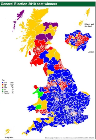
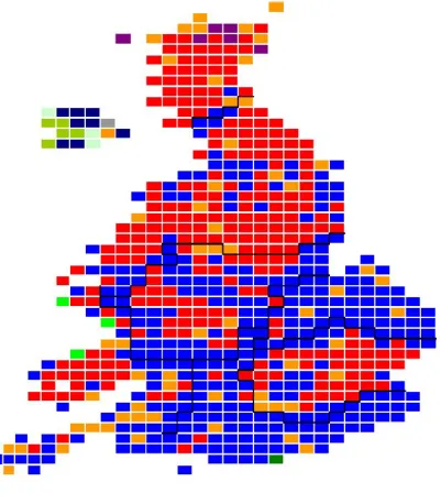
most votes and seats in this particular election. This analysis is further

motivated by the geographic relationships found in maps of the 2010 UK

General Election results, shown in Figures 1 and 2 below. Figures 1 and 2 are

both maps from a House of Commons Briefing paper (HoC, 2010). Figure

1 illustrates the party affiliation of the winning candidate in each of the

UK constituencies (excluding Northern Ireland). Figure 2 shows the same

results in a map where each constituency is represented by an equally-sized

rectangle to mitigate the large differences in geographic area between urban

and rural constituencies. These two maps seem to provide initial evidence

of spatial dependence among the party affiliation of the winning candidate,

given the obvious non-random geographic distribution of the data.

[Insert Figure 1 here]

[Insert Figure 2 here]

The remainder of this paper is organised as follows: Section 2 reviews

voting patterns, Section 3 provides an overview of the data used in this

analysis, and Section 4 presents the baseline ordinary least squares (OLS)

model and results. Section 5 introduces Bayesian spatial econometric models

as an improvement on the OLS model, Section 6 details the results of the

Bayesian model comparison exercise and results from applying the resulting,

most appropriate model, and Section 7 concludes.

2

Literature Review

2.1 The impact of geography on voting outcomes

The impact of environment, or geographical context, on British voting

pat-terns has been acknowledged for many years; the earliest of which may be

Butler and Stokes (1969). They found evidence that constituencies with a

larger proportion of working class people tended to disproportionately show

support for the British Labour Party–providing anecdotal evidence to

sup-port the hypothesis that a voter’s environment does impact voting outcomes

(Butler and Stokes, 1969: 146-150). Their findings are consistent with the

three components of geographical context for elections highlighted in Agnew

(1987: 5):

1. Locale, i.e. the setting for routine social interaction.

2. Location, i.e. the role of the place in the world economy.

3. Sense of place, i.e. the socialization that comes with living in a place.

In explaining UK voting behaviour, it seems logical to expect that 1)

this paper, 2) is harder to motivate since the role of the place in the world

economy is fairly constant across the UK (e.g. there are no differences in

trade laws or currencies). However, upon reflection and in light of the recent

economic downturn affecting the world economy, it could perhaps be argued

that parts of the UK that are more dependent on world trade have been

disproportionately affected. Living in areas experiencing larger effects from

this downturn could have affected voters’ decisions in a different way than

living in areas less affected by the global recession. A report published in

November 2008 by the Local Government Association for England (LGA,

2008) provides some evidence for such regional variation in impacts from

the global recession. The report concluded that, “the projected local

vari-ations from the national average performance are very marked” and “very

strong variations in [economic] performance are likely within individual

re-gions”(LGA, 2008:iii). Not only do they observe regional variations, but

also localised variations within regions. A report by the Institute for Public

Policy Research (IPPR, 2009) makes the same argument. Their report goes

further and suggests that these asymmetric impacts are driven by increased

unemployment, fuelled by redundancies in low value-added manufacturing

industries that are facing competitive pressures from emerging economies

that have a clear cost advantage (IPPR, 2009:10).

The literature on the relationship between the health of the economy

and voting decisions is vast (see for example, Kramer, 1971; MacKuen et

al., 1992; Pacek and Radcliff, 1995; and Sanders et al. 2001). There is

some existing evidence (e.g. Owens and Wade, 1988) that suggests that

in the UK. A similar effect is established for Sweden by Elinder (2010),

who finds that local economic conditions did affect support for the Swedish

government between 1985 and 2002. Similarly, Hellwig (2001) finds that

while accounting for the “exposure” of the domestic economy to the world

economy acts to offset the impact of domestic economic differences in

ex-plaining voting behaviour, these impacts are tied to occupational differences

(Hellwig, 2001:1156).

Given the degree of geographical differentiation in the composition of

the UK economy, examining voting behaviour in a manner that accounts for

spatial differences, as we do in this paper, is a valuable exercise. Other

au-thors seem to agree that considering space when examining voting behaviour

is important. For example, Pattie and Johnston (2000) and O’Loughlin et

al. (1994) argue that socio-economic variables alone are insufficient in

ex-plaining electoral behaviour and that it is important to include locational

effects as well. O’Loughlin et al. (1994) list a number of other studies which

demonstrate the importance of geographic context in explaining electoral

outcomes. Studies listed include one which focuses on Italy (Agnew, 1987),

another which focuses on Scotland (Mercer and Agnew, 1988), and a final

one which analyses the southern United States (Johnston, 1991). All of

these studies tend to emphasise the role played by history and shared

soci-etal experience in understanding spatial variations in electoral outcomes.

There is also a wider literature examining the effect of differing

geo-graphic neighbourhoods on election outcomes. One sub-section of this

liter-ature looks specifically at racial makeup as one aspect of the neighbourhood.

on white voter behaviour. He finds that living in an area with a higher black

voter density increases the chance that a white voter will vote for a black

candidate. A similar effect is recorded by Branton (2004) who finds that

living in a racially diverse community makes voters less likely to support

initiatives in ballots that burden minorities (Branton, 2004:309). These

re-sults are the opposite of those found in two earlier studies, Schoenberger

and Segal (1971) and Wright (1976), both of whom argue that living in an

area with a larger black population increased the proportion of the vote

for the pro-segregationist George Wallace in the US Presidential election of

1968. These studies by no means exhaust the literature on racial context

and voting outcomes, but they are intended to give a flavour of the analyses

that have been undertaken.

Others examine the many aspects of the neighbourhood as a whole.

Pat-tie and Johnston (2000) look at micro-level data for the 1992 UK General

Election and conclude that voters in the UK are influenced both by local

neighbourhood effects and by the political beliefs of those around them,

particularly where these people are family members with whom they

dis-cuss politics (Pattie and Johnston, 2000:62). Burbank (1997) goes further,

examining how a voter’s local level context impacts individual level voting

behaviour. Another study, Macallister et al. (2001), examines voting

be-haviour in the 1997 UK General Election and finds very strong evidence of

a neighbourhood voting effect.

Despite a significant literature existing on neighbourhood effects, we

find that most authors imply that these effects stop at the boundary of the

articles, the characteristics of a constituency affect only that constituency’s

behaviour. Our hypothesis is that there is a more complex system of spatial

interaction that affects voting behaviour. The purpose of our paper, in

part, is to demonstrate this by using the approach outlined in the following

sections. We can then consider the different spatial effects that are involved

in, and help to explain, the observed voting behaviour in the 2010 UK

General Election. By establishing the presence of a spatial dimension in

voting behaviour, we demonstrate that the neighbourhood effects discussed

by others do indeed extend beyond constituency boundaries.

2.2 Spatial Econometric Voting Analysis

We propose to build on the existing analyses relating a voter’s environment

and voting behaviour to assess the strength of these environmental effects

using a spatial econometric model. Before outlining our modelling approach

in Section 4, we first summarise the existing applications of spatial

econo-metric and statistical techniques that analyse voting behaviour. Perhaps

the earliest voting analysis that considers space is Kirby and Taylor (1976).

They examine the spatial pattern of votes cast in the 1975 UK

referen-dum on whether or not to join the European Economic Community, now

the European Union. The vote itself was a straightforward yes/no

refer-endum. While their analysis is not consistent with the spatial econometric

methodology employed here, they did recognise and attempt to model a

spatial dimension in observed voting behaviour. Their analysis divided the

UK into 23 regions and computed two “factor” variables - “core-periphery”

variables. These factors are then included in a linear regression analysis.

Developments in the literature suggest that the regression results obtained

in Kirby and Taylor (1976) may be unbiased but inconsistent (e.g. Barry

et al., 1998). This early work recognised, but could not prove, what we

attempt to establish in this paper - namely that UK voting patterns exhibit

spatial dependence.

Kohfeld and Sprague (1995) examine two elections for citywide offices

in St. Louis, Missouri using a spatial contiguity matrix and the residuals

from a prior non-spatial regression analysis to determine the existence and

strength of spatial dependence in voting behaviour. They conclude that

spatial dependence in voting existed and was quite strong in both elections.

Others make use of an element of exploratory spatial data analysis

-the Moran’s-I statistic - to examine -the existence of spatial dependence in

voting analyses. Seabrook (2009) and Kim, Elliot, and Wang (2003) examine

spatial dependence in US Presidential elections using the Moran’s-I statistic.

Given the similarity in the two approaches, we only discuss the approach of

Seabrook (2009) here. The interested reader is referred to Kim, Elliot, and

Wang (2003) for further details and specific results. Seabrook (2009) uses

this approach to analyse the 2004 and 2008 US Presidential elections. He

measures the degree of homogeneity across counties according to both the

percentage of votes cast for the Democratic candidate and the percentage

of votes cast for the Republican candidate. Seabrook finds that there are

strong and statistically significant levels of positive spatial autocorrelation

in the votes cast for both parties (Seabrook, 2009:4). He also shows that

and 2008.

There are even fewer analyses of voting behaviour that employ more

recent spatial econometric techniques (see LeSage and Pace (2009) for a full

overview of these techniques). There are two notable exceptions: Lacombe

and Shaughnessy (2007) and Cutts and Webber (2010) whom both estimate

a series of spatial econometric models for voting behaviour.

Lacombe and Shaughnessy (2007) analyse US voting behaviour by

ex-amining the 2004 US Presidential election. They argue that despite a

sig-nificant amount of effort being spent on identifying the variables that

in-fluence electoral decisions, the variables that are almost always omitted are

those that differ across space (Lacombe and Shaughnessy, 2007:484). This

omission can result in spatially correlated regression residuals, which lead

to misleading regression coefficients and inferences. They demonstrate the

importance of accounting for spatial dependence in voting analyses by

com-paring the results of a spatial error model with those from a standard OLS

regression. They conclude that OLS regression results based on spatially

autocorrelated data are unbiased but inefficient. Due to a downward bias

in the standard errors, the use of OLS regression techniques on spatially

autocorrelated data can lead to incorrect inferences from the results (e.g.

Lacombe and Shaughnessy, 2007:492 and Barry et al., 1998).

Cutts and Webber (2010) employ several regression analyses (both

non-spatial and non-spatial) in addition to the Moran’s-I statistic to examine vote

share for all major parties in the 2005 UK General Election. Although

like-lihood ratio tests indicate that models which account for spatial dependence

of the coefficients in these spatial regressions may be misleading, in that

they neglect to calculate the direct, indirect, and total effects as developed

by LeSage and Pace (2009).

As a final note, LeSage and Dominguez (2010) look at spatial spillover

effects in the context of public choice issues. Although they examine a

public choice issue related to voting, they do not analyze voting patterns

as we do here. However, LeSage and Dominguez (2010) do demonstrate

the need to take the spatial dimension into account when analyzing such

issues. By examining the impacts of demographic change on local service

provision, they show that increased spending is associated with higher own

county marginal tax cost. In addition, they demonstrate that there is a

spillover effect, which implies that higher spending in one county increases

the marginal tax cost of neighbouring counties. They attribute this result to

“mimicking” behaviour in neighbouring counties where increases in county

service provision create pressure for similar increases in nearby counties.

The interested reader is referred to LeSage and Dominguez (2010) for more

details on their method and other public choice issues examined.

3

Data

The data used in this paper come from a number of different sources. The

primary data source is from a database collected and published online by Dr.

Pippa Norris of Harvard University, available athttp://www.pippanorris.

com/. The dataset used in this study is “May 6th 2010 British General

were a number of seats in which the constituency boundaries changed

sig-nificantly between 2005 and 2010. Due to these changes, many independent

variables that could have been used in this analysis are not yet available for

the 2010 boundary definitions. For example, at the time of this analysis,

data on income and education variables are only available for the 2005

con-stituency boundaries. For consistency, all of the data subsequently used in

this analysis are those available at the 2010 constituency boundaries, and

all are studentized, whereby each variable is transformed by subtracting its

mean and dividing by its standard deviation.

Additional variables were obtained for the unemployment benefit claimant

count from the National Online Manpower Information Service (NOMIS)

website, accessible at https://www.nomisweb.co.uk/Default.asp. This

website is a result of collaboration between the UK Office of National

Statis-tics and the University of Durham and provides statisStatis-tics on the UK Labour

Market. The NOMIS dataset accessed and used in this paper is “claimant

count - age and duration”. This dataset is used to provide a measure of

long-term unemployed (taken as those who have been claiming benefits for

more than 1 year) as a proportion of total claimants in each constituency.

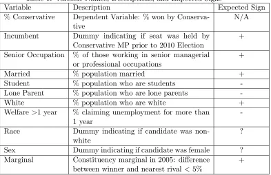
Descriptions of each variable, along with descriptive statistics and the

ex-pected coefficient signs are presented below in Table 1.

We obtained the geographical data for the spatial weight matrix from

the Ordnance Survey website, using the product “Boundary Line”1. This product provides detailed geographic information on the boundaries of each

1

of the UK Parliamentary constituencies as in force on May 6th, 2010. In

all model specifications, we use a contiguity weight matrix based on

Delau-nay triangles. For these 630 UK Parliamentary constituencies, the average

number of neighbors is 6.

It should be noted that we chose to exclude the 18 constituencies in

Northern Ireland from our analysis as the UK Conservative Party does not

directly field candidates in Northern Ireland. Instead, there is an electoral

alliance with the Ulster Unionist Party (UUP) who field candidates with

the understanding that any elected UUP Member of Parliament will take

the Conservative Party whip and could serve in a Conservative Government

(Porter, 2010). We also exclude two additional constituencies from our

anal-ysis: Thirsk & Malton and Buckingham. The election in Thirsk & Malton

was delayed by three weeks due to the death of the UK Independence Party

candidate during the election campaign. As such, we excluded this

con-stituency to focus our analysis on votes that were cast simultaneously. The

seat of Buckingham was excluded as it was the seat of the sitting Speaker

of the House of Commons, John Bercow MP. By convention, the Speaker

is not contested by any of the three main parties when seeking re-election

(HOC-IO, 2010). Our analysis was therefore carried out using data on the

remaining 630 UK Parliamentary constituencies.

[Insert Table 1 here]

As for our prior expectations, given the well known advantages of

the percentage of the vote won by the Conservative candidate. Also, given

that the Conservative Party had high profile initiatives to help married

cou-ples and to limit immigration, we expect that the higher the percentage of

the constituency population that is married, the higher the percentage

Con-servative vote. Similarly, the higher the percentage of the constituency

pop-ulation that is white (and conversely, the lower the non-white poppop-ulation),

the higher the percentage Conservative vote. Other high profile policies,

such as maintaining or increasing student tuition fees, as well as reducing

benefits for those who refuse jobs offers, lead us to expect that the more

stu-dents and the larger percentage of long term unemployed in a constituency,

the lower the percentage vote for the Conservative Party. Also, given the

Conservative Party pledge to scale back some of the tax credits which gave

financial assistance to lone parents, we expect that the more lone parents

there are in a constituency, the lower the percentage Conservative vote. On

the expected sign of some other variables, such as the race and sex of the

Conservative candidate and whether the seat is a marginal seat, we are

gen-uinely undecided and could posit either a positive or negative relationship

between these explanatory variables and the dependent variable.

4

Benchmark OLS Results

To provide an initial baseline regarding the effects of our set of independent

variables on the percentage of the Conservative vote, an OLS regression

y = Xβ+ε (1)

ε ∼ M V N0, σ2In

whereyis ann×1 vector of observations on the percentage of votes cast

for the Conservative Party,Xis ann×kmatrix of economic, socio-economic

and political variables,β is a k×1 vector of coefficient estimates, andε is

ann×1 vector of i.i.d. errors that are distributed multivariate normal with

mean 0 and variance-covariance matrixσ2In.

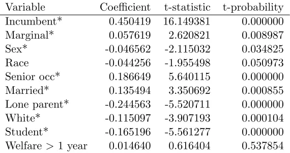
As previously noted, we studentized the dependent variable, as well as

the matrix of independent variables, by subtracting the mean and dividing

by the standard deviation, leading to standardized variables2. The results from the OLS model are given in Table 2. We find that all of the independent

variables are statistically significant at the 5% level, with the exception of the

race variable (significant at the 10% level), and the welfare>1year variable,

which is not statistically significant at any reasonable level.

In terms of our a priori hypotheses regarding the signs of the

coeffi-cient estimates, we find mixed evidence. For example, the seat being held

by a Conservative MP in the last Parliament has a positive effect on the

percentage votes received by the Conservatives. This confirms our initial

expectations about the power of incumbency. The candidate sex and

can-didate race variables have negative coefficients, indicating that where the

2

Conservative candidate was female or of non-Caucasian race, there was a

lower vote for that Conservative candidate. This result is particularly

inter-esting in the context of the recent UK debates about increasing the number

of women and minorities who stand for Parliament. However, it is difficult

here to determine causality. It may be the case that there is a selection issue

in which, women and minorities may, on average, be selected as

Conserva-tive candidates for seats where the ConservaConserva-tive vote is lower, rather than

that the presence of a woman or minority Conservative candidate depresses

the Conservative vote. This perhaps provides one interesting area for future

examination.

Other variables do not conform to our expectations, namely the white

and welfare>1year variables. The percentage of the population that are

white has a negative effect on the percentage of the vote obtained by the

Conservative candidate. This implies that as the percentage of the

popula-tion who are white increases, there is a decrease in the percentage of votes

cast for the Conservative candidate. Given the Conservatives pledged to put

a cap on immigration, as well as their general perception of being tougher

on immigration issues than the other two main parties, we expect their

sup-port to be strongest where the immigrant population is low. It is worth

noting here than an opinion poll, carried out by the polling agency YouGov

for the UK Daily Telegraph newspaper in 2009, found that a majority of

those polled thought that the anti-immigrant British National Party “had

a point” and were correct to “speak up for the interests of the indigenous,

white British people”(Thompson, 2009). In this context, it can perhaps be

who are white are expected to be more supportive of parties, like the UK

Conservative Party, who are seen to be tougher on immigration than the

other main parties. The overall fit of the OLS model is fairly good, with an

adjustedR2 _{of approximately 70%.}

5

Bayesian Spatial Econometric Models

Given the geographic nature of the data, it is reasonable to suspect that

spatial autocorrelation may be an issue. Spatial autocorrelation is formally

defined as follows (Anselin and Bera, 1998):

cov (yi, yj) =E(yi, yj)−E(yi)E(yj)6= 0 f or i6=j (2)

where,yiandyjare observations on a random variable at locationsiand

jin space. The subscriptsiandjcan refer to any geographic designation and

the equation implies non-independence of the random variable across space.

Spatial autocorrelation can pose problems when using standard econometric

techniques, such as OLS.

Spatial econometric models come in three basic varieties, the spatial

autoregressive (SAR) model, the spatial error (SEM) model, and the spatial

Durbin model (SDM). The SAR model can be represented as follows:

ε ∼ M V N0, σ2In

where y is an n×1 vector of observations on the dependent variable,

X is an n×k matrix of independent variables, εis ann×1 vector of i.i.d.

errors, ρ is a scalar spatial autocorrelation parameter, β is a k×1 vector

of regression parameters, and W is an n×n row-stochastic spatial weight

matrix.

The SAR model is used when one believes that spatial autocorrelation is

exhibited in the dependent variable. In our particular empirical application,

it may be that voters across constituencies share common characteristics

regarding voting preferences. Therefore, their votes would be

geographi-cally correlated. It may also be that voters engage in “copy-cat” behavior,

where voters across geographic space mimic each other’s voting preferences.

Regardless of the rationale for the spatial autocorrelation in the dependent

variable, from an econometric perspective, if the true data generating

pro-cess (DGP) for the data is the SAR model, and one uses OLS for estimation

purposes, the resulting coefficient estimates will be biased and inconsistent

due to the endogeneity of theρW y term on the right hand side of the

equa-tion (LeSage and Pace, 2009).

Another variety of spatial econometric model is the SEM model. This

model posits that the spatial autocorrelation is found in the error term and

can be represented mathematically as follows:

u = λW u+ε

ε ∼ M V N0, σ2In

where y is an n×1 vector of observations on the dependent variable,

X is an n×k matrix of independent variables, εis ann×1 vector of i.i.d.

errors, λ is a scalar spatial autocorrelation parameter, β is a k×1 vector

of regression parameters, and W is an n×n row-stochastic spatial weight

matrix.3 It is possible that for a variety of reasons, when an econometric model is specified and estimated, certain factors that should be included in

the model are not and that these factors are correlated over space, resulting

is residual spatial error correlation. In our application regarding

Conserva-tive votes, there may be omitted spatially correlated variables such as shared

cultural norms, media exposure, or other social phenomenon that are either

not quantitatively expressible and/or impossible to proxy for in any

quan-titative or qualitative sense. Additionally, it may be that the constituency

boundaries cut across natural communities, resulting in spatial

autocorre-lation. Or, as is common in the UK, there may be services that are shared

by multiple constituencies; one example of this would be hospital

manage-ment.4 If the true DGP is the SEM model and we use OLS which fails to account for this spatial dimension, the OLS estimators of the coefficients are

unbiased but inefficient and the estimates of the variance of the estimators

3_{Technically, the SEM model illustrated in the text is a spatial error model with} au-toregressive errors. The other, less often used SEM model is the spatial error model with moving average errors.

are biased (LeSage and Pace, 2009). In practice, this can lead to incorrect

inferences regarding the statistical significance of independent variables, and

thus lead one to believe that an independent variable is explaining variation

in the dependent variable when it is actually not.

A final spatial econometric model, a basic extension of the SAR model,

labeled the spatial Durbin model, is mathematically expressed as follows:

y = ρW y+Xβ+W Xθ+ε (5)

ε ∼ M V N0, σ2In

where y is an n×1 vector of observations on the dependent variable,

X is an n×k matrix of independent variables, εis ann×1 vector of i.i.d.

errors,ρis a scalar spatial autocorrelation parameter,β is ak×1 vector of

regression parameters,θis a vector of regression parameters on the spatially

weighted W X variables, and W is an n×n row-stochastic spatial weight

matrix.

The difference between the standard SAR model described above and

the SDM model is the inclusion of spatially weighted independent variables.

LeSage and Pace (2009) show that the SDM model should be used when one

believes that there may be omitted variables that follow a spatial process

and are correlated with included independent variables.

In our empirical application, it is likely that there are some omitted

vari-ables that we are not likely to be able to control for in our empirical

correlated omitted variables are correlated with an included independent

variable, LeSage and Pace (2009) show from a theoretical perspective that

the spatial Durbin model is the most appropriate model.5 One example of such a variable is media outlets/media coverage which is especially relevant

in this particular election because it was the first to televise political

de-bates. Newspapers and other print media are additional examples of media

outlets that we are unable to control for in a meaningful way but that may

be spatially correlated as they tend to service specific geographic areas.

For example, those employed in senior occupations are also consumers

of certain types of media, perhaps business journals or other “conservative”

media outlets. As another example, students may consume different types

of media services, relying on “alternative” media outlets that reflect their

particular political world–view. Again, if these media variables are unable

to be properly entered into our estimating equation and these variables are

correlated with the included variables, we have a strong theoretical case for

use of the spatial Durbin model.

As another example, consider individuals who may be members of

cer-tain civic groups, such as the Rotary Club or other organizations with a

specific agenda. More than likely, membership in these organizations is

spa-tially correlated in that members are most likely from a certain concentrated

geographic area. Since membership information for these groups is

unavail-able, it represents an omitted variable in our econometric specification that

is spatially correlated. This omitted variable is also extremely likely to be

correlated with one of our included explanatory variables, notably the

per-5

centage of the constituency that are in senior occupation fields. Given these

two facts, namely that we have an omitted variable that is spatially

corre-lated and that is also correcorre-lated with an included explanatory variable, we

have another strong argument for using the spatial Durbin model.

Recall that the Parliamentary constituency boundaries changed

signifi-cantly between the 2005 General Election and the 2010 UK General Election.

Independent variables that are not yet available for the new constituency

boundaries, such as income and education level, may also represent

omit-ted variables that are correlaomit-ted with included variables and exhibit spatial

autocorrelation.

Our motivation for using Bayesian spatial econometric techniques, as

opposed to the more familiar maximum likelihood paradigm, is that the

Bayesian paradigm allows one to make non-nested model comparisons in a

statistically coherent manner. Given this advantage, we now turn to the

sta-tistical development of the Bayesian variants of spatial econometric models

and Bayesian model comparison.

By way of notation, letθdenote a vector of parameters of interest,π(θ)

the prior probability density function (pdf) for θ, and let f(y|θ) represent

the likelihood function. The posterior distribution of the parameters, namely

π(θ|y), is derived via Bayes’ Rule:

π(θ|y) = π(y|θ)π(θ)

π(y) (6)

probability density integrates to unity.6

Given thatπ(y) does not involve the parameter vectorθ, we can ignore

this constant in subsequent analyses and write Bayes’ Theorem in a familiar

form:

π(θ|y)∝π(y|θ)×π(θ) (7)

thus resulting in the familiar Bayesian phrase, “the posterior is

propor-tional to the likelihood times the prior”. Ideally, we would like to draw

inferences regarding the parameters of the model by analytically integrating

the joint posterior distribution for each of the model’s parameters, resulting

in a marginal distribution for each parameter. However, the analytical

so-lution to this integration problem is available only in a few select cases. In

deriving the marginal distributions, these complications force us to draw

in-ferences using iterative procedures, referred to generically, as Markov Chain

Monte Carlo (MCMC) methods. Specifically, we will make use of the Gibbs

sampler and the Metropolis-Hastings algorithm to provide robust inferences

regarding the model parameters.

The Gibbs sampler is an algorithm used to generate a sequence of

sam-ples from the joint posterior distribution of the parameters when an

analyt-ical solution is unavailable. There are two necessary conditions for Gibbs

sampling the SAR, SEM, or SDM model, or any model, for that matter.

First, the full conditional distributions comprising the joint posterior must

be available in closed form. Second, these forms must be tractable in the

sense that it is easy to draw samples from them. In terms of the regression

coefficients, represented by thek×1 vector β, these requirements are met

in that random draws from the multivariate normal distribution are used to

obtain parameter estimates. This is also true in terms of the error variance

parameter,σ2, whereby inferences are obtained via random draws from the inverse Gamma distribution. The only full conditional distribution that does

not fall into this category is the spatial autocorrelation parameter,ρ, which

must employ a relatively straightforward random–walk Metropolis–Hastings

algorithm.

The Metropolis-Hastings algorithm is an accept-reject type algorithm

in which a candidate value is proposed and then one decides whether to set

the next value of the chain equal to this proposed value or to remain at the

current value. The Metropolis-Hastings algorithm mimics the Gibbs

sam-pling algorithm but the difference is that the Metropolis-Hastings algorithm

can be used for conditional distributions that do not have any recognizable

distributional form. If the Metropolis-Hastings algorithm is used in

com-bination with standard Gibbs sampling techniques, it is referred to as the

“Metropolis-within-Gibbs” method. Further mathematical and

computa-tional details regarding MCMC estimation of spatial econometric models is

covered in LeSage and Pace (2009) and Lacombe (2008).

The formula for Bayes’ Rule explicitly allows for prior information to

be included in the statistical analysis. In each of our models, we use proper

prior distributions, but with fairly uninformative values. Specifically, we set

mean ˆβ ≡0K and covariance C_βˆ≡10,000×IK. The prior values for theσ

parameter, which comes from the inverted Gamma distribution, areυ0 ≡1

and s2₀ ≡ 1 and the prior values for the ρ term comes from a univariate normal prior, with meanρ0 ≡0 and standard deviation 10,000.

Another appealing aspect of Bayesian analysis is the formal statistical

derivation of model comparison techniques. In the empirical application that

follows, we were uncertain about which model is the correct one, i.e. SAR

vs. SEM vs. SDM. We solve this problem by calculating posterior model

probabilities and choosing the best model based on these calculations.7 The essential inputs in Bayesian model comparisons are the marginal likelihoods

of competing models. As previously mentioned, the marginal likelihood,

de-notedπ(y), is the integrating constant that ensures that the posterior

distri-bution integrates to unity. Until recently, the computation of the marginal

likelihood has proved to be extremely burdensome for all but the simplest

models. In our model comparison exercise, we use the marginal likelihood

calculation as outlined in Chib and Jeliazkov (2001), which is an extension of

the algorithm proposed in Chib (1995) for models that include a Metropolis–

Hastings step. The marginal likelihood can be used to calculate posterior

model probabilities according to the following formula:

π(Mi|y) =

π(Mi)π(y|Mi) J

P

j=1

π(Mj)π(y|Mj)

(8)

where π(Mi|y) is the posterior probability of model i, π(Mi) is the

prior probability of model i , and π(y|Mi) is the marginal likelihood for

modeli , where{M1, . . . , MJ} denotes each of theJ models. Model choice

then proceeds by choosing the model with the highest posterior probability.

6

Results

The posterior model probabilities for each of the 3 models are given in Table

3. We ran each of the 3 models for 20,000 iterations using the initial 10,000

iterations as “burn in” of the sampler, and assumed that each model was a

priori equally probable, i.e. π(Mi) was equal to 1/3 for each model. The

results from our Bayesian model comparison exercise indicate that the most

preferred model is the spatial Durbin model, with a posterior probability of

approximately 100%. This empirical finding is in accordance with our

previ-ous theoretical discussion regarding the appropriateness of using the spatial

Durbin model when one believes that there are omitted variables that are

spatially correlated and that are correlated with included explanatory

vari-ables. Given such a high posterior model probability, as well as theoretical

considerations, we limit our discussion to the results of the spatial Durbin

model.

In our spatial model, as is the standard practice in Bayesian regression

analyses, we calculated 95% credible intervals from the Gibbs samples for

the regression coefficients. Those intervals that do not contain zero are

considered “significant” in the sense that the variable is associated with

is followed by a * in Table 4, the respective coefficient on that variable is

associated with the dependent variable at the 95% level, i.e. the 95% credible

interval points to a posterior distribution for the parameter estimate that is

far enough away from zero which gives credence to an important role played

by these variables in explaining the percentage of Conservative votes.

We begin our discussion of the regression results by noting that the

spatial autocorrelation coefficient,ρ, has a value of.6977 and a 95% credible

interval of [.6318, .7614] meaning that there is a 95% probability that the

true value of ρ lies within this interval. We also note that the value of ρ

indicates a moderate to high level of spatial autocorrelation in our dependent

variable.

LeSage and Dominguez (2010) argue that directly comparing OLS β’s

andβ’s from a spatial autoregressive (SAR) or spatial Durbin (SDM) model

is inappropriate due to the fact that the coefficients in an OLS regression

model accurately measure the effect of a change in an explanatory variable

on the dependent variable, while a SAR or SDM model’s coefficients “are

not directly interpretable with regard to how explanatory variables in the

model influence the dependent variable” (LeSage and Dominguez, 2010:4).

We follow LeSage and Pace (2009, Chapter 2) and calculate the direct,

indirect, and total effects estimates in regards to each of our independent

variables.

The first thing to note is that all of the signs on our statistically

signif-icant independent variables are in accordance with our prior expectations,

a marked difference from our benchmark OLS model. For example, in the

contrast to our expectations. The SDM model, without exception, exhibits

coefficient signs that are in accordance with our hypothesized signs, as well

as political and economic theory.

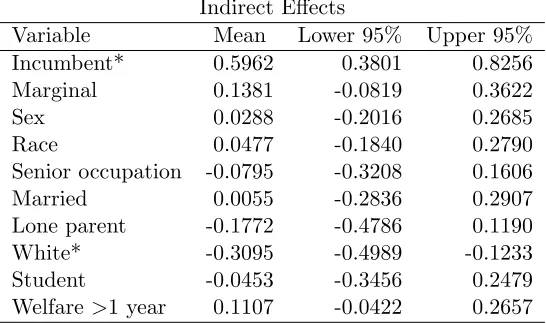
Table 4 shows that the incumbent variable has a positive and significant

direct, indirect and total effect on the percentage of the vote obtained by the

Conservative candidate. This result is in line with the commonly understood

advantages incumbents have over challengers including name recognition,

ac-cess to public funding as part of the MPs communications allowance, and

a record in office on which to campaign. The positive and significant

indi-rect effect suggests that there is an important impact that incumbent MPs

can have in increasing their parties support in neighbouring constituencies.

There are a number of reasons that could help explain this effect; for instance

an incumbent has both resources and staff available to publicise themselves

in the media (a medium that does not respect constituency boundaries).

Similarly, there may be local issues on which incumbents may have

“own-ership”, but which affect neighbouring constituencies as well (for example

hospital closures or policing issues). Another explanation could stem from

the fact that an incumbent MP is a full time advocate for their party in

the community, and that part of this role is (implicitly or explicitly) to

pro-mote their party in neighbouring constituencies (including for example, by

mentoring the party’s candidates for neighbouring seats) which are currently

held by other parties. Whatever the reason, the existence of such an effect is

interesting and helps us to better understand the full effects of incumbency

beyond the narrow focus of increasing the re-election chances of the

of “foothold effects” where a party that managed to gain a foothold in a

hitherto unwinnible area may be able to use this initial gain to spur a wider

increase in their party’s support, although it may have been the same effect

(operating in favour of the opposition party) that led the area to become

unwinnable in the first place.

The positive and significant coefficients on the direct effects of the senior

occupation and married variables are also expected. The high profile pledge

made by the Conservative Party to recognize marriage in the tax system

(Watt, 2010) and the introduction by the incumbent Labour government of

a top income tax rate of 50% (BBC News, 2009) – which the Conservatives

indicated they would repeal once the economy recovered (Conservative Party

Website, 2010) – seem to help explain our findings here. Neither of these

variables has a significant indirect or total effect, suggesting that the effect

of the proportion of the the local population in these groups is limited to

“within” the constituency. This is a reasonable result since it is difficult

to conceive how an increase in the number of married couples or senior

managers in one constituency could have an effect on the level of support

for a political party in a neighbouring constituency.

The direct effects of the student and lone parent variables seem to be

reflecting the fact that these are “non-core” Conservative voting groups

and despite recent attempts by the UK Conservative Party to “woo” these

groups, these results indicate that where these groups are more populous in

a constituency, they exert a negative effect on the percentage of the votes

cast for the Conservative candidate. Arguably, the biggest issue currently

fees for university education. The Conservatives claimed that they would

keep tuition fees, unlike their Liberal Democrat opponents (and subsequent

coalition partners) who pledged to fight to remove them (Grimston, 2010).

It is perhaps not a surprise that a party pledging to keep university fees

in place, and even to increase them, would not find favour with students.

Indeed, an opinion poll conducted in the UK in April 2010 showed that

some 68% of students surveyed would be less likely to vote for a party that

planned to increase tuition fees (Endsleigh, 2010). Similarly, there was a

suggestion that the recognition of marriage in the tax system that

Conser-vatives proposed would hurt single-parent households (Walker, 2009). This

may explain, in part, our findings that the more lone parents there are in a

constituency, the lower the percentage of the vote won by the Conservative

Party.

The next variable of consequence is the white variable, which has a

positive and significant direct effect coefficient suggesting that the higher

the percentage of the population that is white, the higher the percentage

Conservative vote. The indirect effect estimate for this variable is also

signif-icant, but negative. This result implies that the higher the proportion of the

population that are white in one constituency, the lower the support for the

Conservative Party in neighbouring constituencies. Conversely, the lower

the percentage of the population in one constituency who are white, the

higher the support for the Conservative Party in neighbouring

constituen-cies. The latter explanation is consistent with cases of community tensions

surrounding constituencies with a particularly high level of non-white

population that is non-white (perhaps composed of a number of current

asylum seekers) could create cohesion issues around shared amenities. This

may result in voters in neighbouring constituencies increasing their support

for parties that are considered to be tougher on immigration issues. We

provide no support here for any particular direction of causality and are

merely speculating as to the cause of this effect. Perhaps the most

interest-ing aspect of the results relatinterest-ing to the white variable is that the size of the

negative indirect effect easily dominates the positive direct effect, resulting

in a negative and significant total effect.

The welfare variable has a negative and significant direct effect

coeffi-cient implying that the higher the percentage of benefit claimants who are

considered “long term”, the lower the percentage Conservative vote. This

result is not surprising in light of the high profile campaign the

Conserva-tives ran to cut benefits for unemployed people who refuse offers of work

(Shipman, 2010). The indirect effect estimate is insignificant, as is the total

effect estimate.

The marginal variable, which is a dummy variable indicating that the

gap between the first and second place candidates in the previous 2005

UK General Election was <5%, has a positive and significant direct effect

estimate. This suggests that the percentage of the Conservative vote was

higher where the race was closer. This could suggest that the Conservative

voters are more responsive to the closeness of the race, perhaps recognising

7

Conclusion

We set out to test two principle research questions, 1) whether or not there

is spatial dependence in the votes cast for the Conservative Party in the 2010

UK General Election and 2) what economic, socio-economic, and political

factors help explain the variation in the percentage of the vote won by the

Conservative Party across the UK. Many empirical models of voting

out-comes ignore the effects of spatial dependence, resulting in estimates that

can be biased, inconsistent, or both. To take account of spatial dependence,

we estimated a series of Bayesian spatial econometric models designed to

control for any spatial dependence inherent in the data. We examined three

different spatial econometric models, and used modern Bayesian model

com-parison techniques to produce posterior model probabilities for guiding our

model selection.

On examining the coefficients in the most appropriate model, the

spa-tial Durbin model, we found that almost all of the significant explanatory

variables reinforced our prior beliefs. The incumbent, senior occupation,

married, and white variables all exerted a positive and significant effect on

the percentage of the votes for the Conservatives, while student, lone parent,

and welfare<1 year all exerted a significant negative effect on the percentage

of votes cast for the Conservative Party. Perhaps the most interesting result

from our analysis is that the incumbent variable has a positive and

signif-icant indirect effect. There are a number of possible explanations for this

which were discussed earlier in this paper. What this finding does though,

be-yond the realm of candidate self-preservation and focuses it also on these

indirect effects, which are a potentially interesting aspect of understanding

election outcomes. The full results presented in this paper demonstrate that

controlling for residual spatial autocorrelation is a vital component of any

empirical analysis of voting behavior.

Spatial econometric techniques are garnering more attention in the field

of economics and beyond. The full suite of spatial econometric models that

are now available provide an excellent basis on which to better model and

examine the underlying relationships in datasets like the one used here.

Additionally, the Bayesian statistical paradigm allows one to make

non-nested model comparisons with relative ease and provides a more nuanced

approach to model selection.

Future research will look at the insights that can be gained from looking

at these issues further using different modelling approaches, including

con-sideration of “regional level” effects, where the spatial effects are modeled

as unobserved effects at a regional level.

8

References

Agnew JA (1987)Place and Politics, Boston: Allen and Unwin

Anselin L, Bera A (1998) Spatial dependence in linear regression

mod-els with an introduction to spatial econometrics. In: Ullah A, Giles

DEA (eds) Handbook of applied economic statistics. Marcel Dekker,

Barry R, Pace RK, and Sirmans CF (1998) Spatial statistics and real

estate. Journal of Real Estate Finance and Economics 17(1): 5-13

BBC News (2009) Tax rise as UK debt hits record, BBC News Website,

last updated Wednesday, 22 April 2009, available from: http://news.

bbc.co.uk/1/hi/uk_politics/8011321.stmAccessed: 22 July 2010

Branton RP (2004) Voting in Initiative Elections: Does the Context of

Racial and Ethnic Diversity Matter? State Politics and Policy

Quar-terly 4(3): 294-317

Burbank MJ (1997) Explaining Contextual Effects on Vote Choice

Po-litical Behavior 19(2): 113-132

Butler D and Stokes D (1969) Political Change in Britain (1st.

edi-tion). MacMillan: London

Carsey TM (1995) The Contextual Effects of Race on White Voter

Behavior: The 1989 New York City Mayoral ElectionThe Journal of

Chib, S (1995) Marginal Likelihood from the Gibbs Output Journal

of the American Statistical Association 90(432): 1313-1321

Chib, S and Jeliazkov I (2001) Marginal Likelihood from the Metropolis–

Hastings OutputJournal of the American Statistical Analysis96(453):

270-281

Conservative Party Website (2010) Where we stand: the economy, The

Conservative Party website, available from: http://www.conservatives.

com/Policy/Where_we_stand/Economy.aspxAccessed: 21 July 2010

Cutts D and Webber DJ (2010) Voting patterns, party spending and

relative location in England and WalesRegional Studies44(6): 735-760

Elhorst, JP (2010) Applied Spatial Econometrics: Raising the Bar

Spatial Economic Analysis 5(1): 9-28

Elinder, M (2010) Local economies and general elections: The

influ-ence of municipal and regional economic conditions on voting in

Swe-den 1985-2002European Journal of Political Economy 26(2): 279-292

Endsleigh (2010) Student vote could swing election as a top-up fee

from: http://www.endsleigh.co.uk/Media/Pages/StudentElection2010.

aspxAccessed: 25 August 2010

Grimston J, Labour revolt over tuition fees, The Sunday Times Online,

available fromhttp://www.timesonline.co.uk/tol/news/politics/

article7094316.eceAccessed: 11 April 2010

Hellwig TT (2001) Interdependence, Government Constraints, and

Economic VotingThe Journal of Politics 63(4): 1141-1162

House of Commons (2010)“General Election 2010: Final edition”,

House of Commons Briefing Paper, available fromhttp://www.parliament.

uk/briefingpapers/commons/lib/research/rp2010/RP10-036.pdf

House of Commons-Information Office (2010) “The Speaker”, House

of Commons Information Office Factsheet, M2, available fromhttp://

www.parliament.uk/documents/commons-information-office/m02.

pdf

Institute for Public Policy Research (2009) “The Impact of the

Reces-sion on Northern City-Regions”, IPPR Report, available fromhttp://

www.ippr.org.uk/members/download.asp?f=/ecomm/files/impact_

Johnston RJ (1991)A question of place Basil Blackwell: Oxford

Kirby AM and Taylor PJ (1976) A Geographical Analysis of the

Vot-ing Pattern in the EEC Referendum, 5 June 1975Regional Studies 10:

183-191

Kohfeld CW and Sprague J (1995) Racial context and voting

behav-ior in one-party urban political systems Political Geography 14(6-7):

543-569

Kramer G (1971) Short-Term Fluctuations in U.S. Voting Behavior,

1896-1964The American Political Science Review 65(1): 131-143

Kim J, Elliot E, and Wang D (2003) A spatial analysis of county-level

outcomes in US Presidential elections: 1988-2000Electoral Studies 22:

741-761

Lacombe DJ and Shaughnessy TM (2007) Accounting for Spatial

Er-ror Correlation in the 2004 Presidential Popular Vote Public Finance

Lacombe DJ (2008) An Introduction to Bayesian Inference in Spatial

Econometrics, SSRN Working Paper, available from http://ssrn.

com/abstract=1244261Accessed: 24 July 2010

LeSage JP and Dominguez M (2010) The importance of modeling

spa-tial spillovers in public choice analysis (in press)Public Choice

LeSage JP and Pace RK (2009)Introduction to Spatial Econometrics

CRC Press: Boca Raton

Local Government Association of England (2008) “From recession

to recovery: the local dimension”, Local Government Association of

England Report, available from http://www.lga.gov.uk/lga/aio/

1215871Accessed: 24 August 2010

Macallister I, Johnston RJ, Pattie CJ, Tunstall H, Dorling DFL, and

Rossiter DJ (2001) Class Dealignment and the Neighbourhood Effect:

Miller RevisitedBritish Journal of Political Science 31: 41-59

MacKuen MB, Erikson RS and Stimson JA (1992) Peasants or Bankers?

The American Electorate and the U.S. EconomyThe American

Mercer J and Agnew J (1988) Small worlds and local heroes: the 1987

General Election in Scotland Scottish Geographical Journal 104(3):

138-145

O’Loughlin JV, Flint C, and Anselin L (1994) The geography of the

Nazi vote: context, confession and class in the Reichstag election of

1930Annals of the Association of American Geographers 84: 351-380

Owens JR and Wade LL (1988) Economic Conditions and Constituency

Voting in Great BritainPolitical Studies 36(1): 30-51

Pacek AC and Radcliff B (1995) Economic Voting and the Welfare

State: A Cross-National AnalysisThe Journal of Politics 57: 44-61

Pattie C and Johnston R (2000) People Who Talk Together Vote

To-gether: An Exploration of Contextual Effects in Great BritainAnnals

of the Association of American Geographers 90(1): 41-66

Porter A (2010) David Cameron launches biggest Conservative

shake-up for decades The Daily Telegraph Published: 11:47PM BST 23 Jul

2008, available fromhttp://www.telegraph.co.uk/news/newstopics/

politics/conservative/2450913/David-Cameron-launches-biggest-Conservative-shake-up-for-decades.

Sanders D, Clarke H, Stewart M, and Whiteley P (2001) The Economy

and VotingParliamentary Affairs 54: 789-802

Schoenberger RA and Segal DR (1971) The Ecology of Dissent: The

Southern Wallace Vote in 1968 Midwest Journal of Political Science

15(3): 583-586

Seabrook NR (2009) The Obama Effect: Patterns of Geographic

Clus-tering in the 2004 and 2008 Presidential Elections The Forum 7(2),

Article 6

Shipman T (2010) “Cameron in benefits threat to the workshy as

he declares: ‘The free ride is over’ ”, The Daily Mail Online, Last

Updated: 8:43am on 21st April 2010, available from http://www.

dailymail.co.uk/news/election/article-1267465/General-Election-2010-Cameron-benefits-threat-workshy-declares-The-free-ride-over.

htmlAccessed: 14 July 2010

Thompson D (2009) “Opinion poll: more than half of British voters

think the BNP ‘has a point’ ”, The Daily Telegraph Blogs, Last

up-dated: October 23rd, 2009, available fromhttp://blogs.telegraph.

co.uk/news/damianthompson/100014692/opinion-poll-more-than-half-of-british-voters-think-the-bnp-has-a-point/

Walker K (2009) “Cameron denies ‘war’ on lone parents after

pledg-ing to support marriage through the tax system”, The Daily Mail

online, Last updated 8th December 2009, available fromhttp://www.

dailymail.co.uk/news/article-1233939/Cameron-insists-Tories-support-single-parents-backlash-married-couple-tax-breaks-policy.

htmlAccessed: 12 August 2010

Watt N (2010) “Conservatives commit to 150 tax break for married

couples”, The Guardian website, Saturday 10 April 2010, available

fromhttp://www.guardian.co.uk/politics/2010/apr/10/conservatives-tax-breaks-married-couples

Accessed: 13 July 2010

Wright GC, Jr. (1976) Community Structure and Voting in the South

9

Figures

10

Tables

Table 1: Variable Names, Descriptions, and Expected Signs

Variable Description Expected Sign

% Conservative Dependent Variable: % won by Conserva-tive

N/A

Incumbent Dummy indicating if seat was held by

Conservative MP prior to 2010 Election

+

Senior Occupation % of those working in senior managerial or professional occupations

+

Married % population married +

Student % population who are students

-Lone Parent % population who are lone parents

-White % population who are white +

Welfare>1 year % claiming unemployment for more than 1 year

-Race Dummy indicating if candidate was

non-white

?

Sex Dummy indicating if candidate was female ?

Marginal Constituency marginal in 2005: difference

between winner and nearest rival <5%

Table 2: OLS Results

Variable Coefficient t-statistic t-probability

Incumbent* 0.450419 16.149381 0.000000

Marginal* 0.057619 2.620821 0.008987

Sex* -0.046562 -2.115032 0.034825

Race -0.044256 -1.955498 0.050973

Senior occ* 0.186649 5.640115 0.000000

Married* 0.135494 3.350692 0.000855

Lone parent* -0.244563 -5.520711 0.000000

White* -0.115097 -3.907193 0.000104

Student* -0.165196 -5.561277 0.000000

Welfare >1 year 0.014640 0.616404 0.537854

R-squared = 0.7117 Rbar-squared = 0.7076

Table 3: Model Comparison Results

Model Log-Marginal Likelihood nse Posterior Probability

SAR -310.6830 .1968 ≈0

SEM -482.98 .1969 ≈0

Table 4: Effects Estimates

Direct Effects

Variable Mean Lower 95% Upper 95%

Incumbent* 0.2802 0.2379 0.3238

Marginal* 0.0370 0.0034 0.0712

Sex -0.0345 -0.0695 0.0003

Race -0.0325 -0.0688 0.0036

Senior occupation* 0.1794 0.1189 0.2389

Married* 0.1608 0.0936 0.2289

Lone parent* -0.1016 -0.1729 -0.0288

White* 0.0868 0.0297 0.1444

Student* -0.1161 -0.1658 -0.0659

welfare >1 year* -0.0673 -0.1109 -0.0243

Indirect Effects

Variable Mean Lower 95% Upper 95%

Incumbent* 0.5962 0.3801 0.8256

Marginal 0.1381 -0.0819 0.3622

Sex 0.0288 -0.2016 0.2685

Race 0.0477 -0.1840 0.2790

Senior occupation -0.0795 -0.3208 0.1606

Married 0.0055 -0.2836 0.2907

Lone parent -0.1772 -0.4786 0.1190

White* -0.3095 -0.4989 -0.1233

Student -0.0453 -0.3456 0.2479

Total Effects

Variable Mean Lower 95% Upper 95%

Incumbent* 0.8764 0.6434 1.1228

Marginal 0.1751 -0.0663 0.4178

Sex -0.0058 -0.2574 0.2565

Race 0.0152 -0.2417 0.2731

Senior occupation 0.0999 -0.1548 0.3543

Married 0.1662 -0.1403 0.4650

Lone parent -0.2788 -0.5955 0.0356

White* -0.2227 -0.4172 -0.0311

Student -0.1615 -0.4912 0.1612