City, University of London Institutional Repository
Citation
:
Shafqat, K., Pal, S. K. and Kyriacou, P. A. (2007). Evaluation of two detrending
techniques for application in Heart Rate Variability. Paper presented at the 29th Annual
International Conference of the IEEE Engineering in Medicine and Biology Society, 22-26
Aug 2007, Lyon, France.
This is the accepted version of the paper.
This version of the publication may differ from the final published
version.
Permanent repository link: http://openaccess.city.ac.uk/14301/
Link to published version
:
http://dx.doi.org/10.1109/IEMBS.2007.4352275
Copyright and reuse:
City Research Online aims to make research
outputs of City, University of London available to a wider audience.
Copyright and Moral Rights remain with the author(s) and/or copyright
holders. URLs from City Research Online may be freely distributed and
linked to.
City Research Online:
http://openaccess.city.ac.uk/
[email protected]
Abstract— The performance of two different algorithms of detrending the RR-interval before Heart Rate Variability (HRV) analysis has been evaluated using both, simulated signals and real RR-interval time series. The first algorithm is based on the Smoothness Prior Approach (SPA) and the second algorithm is implemented using Wavelet Packet (WP) analysis. The calculated time and frequency domain parameters obtained from real signals after detrending and the results obtained from simulated signals suggest that the WP method performed better than the SPA. The WP method provided more attenuation of the slow varying trend and was able to preserve the other signal components better than the SPA method. Also the SPA method was computationally slower and it might be not appropriate with long signals.
I. INTRODUCTION
eart Rate Variability (HRV) is widely used as a quantitative marker of the autonomic nervous system activity. Various time domain and frequency domain methods have been used for HRV analysis [1]. The performance of most of these methods was found to be affected by nonstationary, slow varying trends, present in the HRV signal. In particular these nonstationarities will distribute large amount of variance in the lowest frequency.
In order to deal with these nonstationarities many researchers detrend the data prior to the analysis. Detrending is usually based on first order [2], [3] or higher order [3] polynomial model. The polynomial filter presented by Porges and Bohrer [4] is quite sensitive to the choice of polynomial order and the duration. To avoid these problems another method based on the Smoothness Prior Approach (SPA) was purposed [5]. This method is advantageous, as it behaves as a time varying Finite Impulse Response (FIR) high pass filter whose cutoff frequency can be changed by changing one parameter.
This study presents a quantitative comparison between the detrending method based on the SPA and another detrending
Manuscript received April 2, 2007.
This work was supported by Chelmsford Medical Education and Research Trust (CMERT).
K. Shafqat is with the School of Engineering and Mathematical Sciences, City University, London, EC1V 0HB, UK (phone: +44 (0) 20 7040 3878; fax: +44 (0) 20 7040 8568; e-mail: [email protected]).
P. A. Kyriacou is with the School of Engineering and Mathematical Sciences, City University, London, EC1V 0HB, UK (e-mail: [email protected]).
S. K. Pal is with St Andrew’s Centre for Plastic Surgery & Burns, Broomfield Hospital, Chelmsford, CM1 7ET, UK (e-mail: [email protected]).
method implemented using Wavelet Packet (WP) analysis.
II. METHODS
In this work the RR-interval time series was resampled at 4 Hz to obtained equidistance samples using Berger’s algorithm [6]. Before comparing the two methods a brief description of the two approaches will be given in this section.
A. Detrending using Smoothness Prior Approach (SPA)
In this method a N−1 long equidistance heart rate series is represented as
trend stationary z
z
z= + (1)
The estimated stationary part is written as
z D D H
z
zˆstationary ˆ ( ( T ) )
1 2 2
2 −
+ Ι − Ι = −
= θλ λ (2)
Where H∈R(N−1)×M is the observation matrix. For simplification, an identity matrix is used in place of the observation matrix
H
. θˆ represents the estimate of the λ regression parameters with λ as the regularization parameter and D2∈R(N−3)×(N−1) is the second order difference matrix. A detailed description of this method can be found in [5].Equation (2) can be written as zˆstationary =Lz where
1 2 2 2
) (Ι+ −
− Ι
= D D
L λ T corresponds to a time varying FIR highpass filter.
B. Wavelet Packets (WP) detrending method
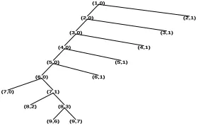
Wavelet packet analysis is a generalization of wavelet analysis offering a richer decomposition procedure by splitting not only the approximation (lowpass) part of the signal, as done in the case of Discrete Wavelet Transform, but also the detail (highpass) part of the signal. The original signal is considered to be at level 1 and the decomposition process is applied n times to get the WP transform at level n + 1. As a result of full WP decomposition of a signal to certain level the filter bank structure becomes a full binary tree.
The detrending algorithm was implemented using Daubechies compactly supported orthonormal wavelet transform method with an order of 12. As mentioned before
Evaluation of two detrending techniques for application in Heart
Rate Variability
First K. Shafqat, Second S. K. Pal and Third P. A. Kyriacou, Senior Member, IEEE
the sampling frequency of the RR-interval time series was chosen to be 4 Hz and therefore, at this sampling rate the basis used in WP analysis to suppress the VLF component of the HRV signal is shown in Fig. 1.
(1,0)
(2,0) (2,1) (3,0) (3,1) (4,0) (4,1) (5,0) (5,1) (6,0) (6,1) (7,0) (7,1)
(8,2) (8,3) (9,6) (9,7)
Fig. 1. WP tree used for detrending. The pair of numbers in the bracket at
each node represent particular part of the decomposition. The first number in the pairs shows the level of the decomposition j and the possible values
for the second number (n) are 0...2(j−1)−1 except for j−1 which
represents the original signal
The performance of both the detrending algorithms was first evaluated using two simulated signals (signals 1 and 2). The algorithms were then tested with real data. The effect of detrending on the time domain analysis was studied using three parameters recommended in [1] and also used in [5]. These parameters include, standard deviation of all RR intervals (SDNN), the square root of the mean squared differences of successive RR intervals (RMSSD) and the relative amount of successive RR intervals differing more than 50 ms (pNN50).
The simulated signals were used to clearly identify the differences in the performance of the two methods. Both simulated signals consisted of three sine wave components corresponding to the Very Low Frequency (VLF), Low Frequency (LF) and High Frequency (HF) components of the HRV signal.
III. RESULTS
The results from each detrending method when analyzing the two simulated signals and the real RR-interval time series (obtained from 4 subjects) will be presented separately in the next sections.
A. Detrending using Smoothness Prior Approach (SPA)
The Fourier transform of the middle row of L (see (2)) is used to calculate the cut-off frequency of the filter [5]. The cut-off frequency of this filter depends on the sampling rate of the signal and the value of λ, and decreases as the value of λ increases. At the sampling frequency of 4 Hz the changes in the cut-off frequency due to the changing values of λare shown in Fig.2.
The first simulated signal (signal 1) used for evaluation of the detrending method consisted of three sine wave components of equal amplitudes at 0.025, 0.045 and 0.18 Hz. In the case of the second simulated signal (signal 2) the frequency corresponding to the slowest component was changed from 0.025 Hz to 0.035 Hz. The frequencies of the
[image:3.612.112.252.115.204.2]other two components remained the same. In order to attenuate most of the signal up to the VLF range a value of 413 was used for λ which made the cut-off frequency of the filter to be approximately 0.0391 Hz. The results obtained from detrending these two simulated signals are presented in Fig. 3.
0 200 400 600 800 1000
0 0.05 0.1 0.15 0.2 0.25
Lambda values
[image:3.612.319.551.130.211.2]Normalized cut−off frequency
Fig. 2. Effect of changes in λ values on the cut-off frequency of the filter
at a sampling rate of 4 Hz. The cut-off values are presented with respect to normalized frequency
Fig. 3(c) and 3(d) shows the detrended signals showing clearly that the slow varying parts of the original signals have been attenuated to some extent. The changes caused by the detrending algorithm in the frequency components of the signals can be seen by looking at the normalized magnitude spectrum of the signals before and after detrending (Fig. 4).
−4 −2 0 2 4
Amplitude (arb. units)
(a) (b)
0 125 255
−4 −2 0 2 4
(c)
0 125 255
(d)
Time (s)
Fig. 3. Results of detrending the simulated signals using SPA method; (a)
simulated signal 1 (thin line) and estimated trend (thick line); (b) simulated signal 2 (thin line) and estimated trend (thick line); (c) detrended signal 1 and (d) detrended signal 2
0 0.125 0.25 0
0.4 0.8 1
Normalized Magnitude
(arb. units)
(a)
0 0.125 0.25 0
0.4 0.8
1 (b)
0 0.125 0.25 0
0.4 0.8
1 (c)
0 0.125 0.25 0
0.4 0.8
1 (d)
Frequency (Hz)
Fig. 4. (a) Magnitude spectrum of the original simulated signal 1; (b)
Magnitude spectrum of the original simulated signal 2; (c) the spectrum of the signal 1 after removing the trend using the SPA; (d) the spectrum of the signal 2 after removing the trend using the SPA
[image:3.612.320.551.330.439.2] [image:3.612.318.547.490.588.2]analysis. For autoregressive spectrum a model order of 20 was used and the coefficients were calculated using modified covariance method. 0.6 1 1.4 0.6 1 1.4
0 300 600 −0.25
0 0.25
RR (s)
0 300 600 −0.35 −0.1 0.25 1.1 1.2 1.3
0 300 600 −0.07 0 0.07 0.67 0.75 0.83
0 300 600 −0.04
0 0.04
TIme (s)
Fig. 5. Top row shows the original RR-interval time series (thin line) and
the estimated trend (thick line) for each subject and the bottom row shows the detrended signal using the SPA
0 0.25 0.5 0
0.05 0.1
0 0.25 0.5
0 0.25 0.5 0
0.025 0.05
PSD (s
2/Hz)
0 0.25 0.5
0 0.25 0.5
0 0.25 0.5
0 0.25 0.5
0 0.25 0.5
Frequency (Hz)
Fig. 6. Power Spectral Density (PSD) of the signal before (lighter line) and
after detrending (darker line) using SPA for the four subjects. Top row shows the results obtained using the non-parametric (Welch’s) method and
the bottom row shows the results obtained using a 20th order AR model
From the spectrum obtained using Welch’s method (Fig. 6 top row) it can be seen that the VLF component has been attenuated considerably with a slight change in the LF region of the signal. More prominent change can be seen by comparing the spectrums obtained using the AR method (Fig. 6 bottom row) before and after detrending. In this case, before detrending the peak around 0.1 Hz can not be distinguished clearly because of the strong VLF component. After detrending, the peak in the LF region, around 0.1 Hz, is clearly visible.
B. Detrending using Wavelet Packet (WP) analysis
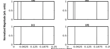
[image:4.612.319.540.59.172.2]The second method used in this study was based on WP analysis. The results obtained by analyzing both simulated signals are shown in Fig. 7. The spectrums of the two simulated signals before and after detrending are shown in Fig. 8.
From Fig. 8(c) and 8(d) it can be seen that WP analysis detrending technique has not only reduced the slow varying component significantly, but also it has not caused any significant reduction in the power of the other two components. The results obtained by WP detrending of the real RR-interval time series of the same four subjects used in Fig. 5 are shown in Fig. 9. The spectrums of the original RR-interval time series and the detrended signals of Fig. 9 are
shown in Fig. 10
−4 −2 0 2 4
Amplitude (arb. units)
(a) (b)
0 125 255
−4 −2 0 2 4 (c)
0 125 255
(d)
[image:4.612.62.281.97.213.2]TIme (s)
Fig. 7. Results of detrending the simulated signals using the WP method;
(a) simulated signal 1 (thin line) and estimated trend (thick line); (b) simulated signal 2 (thin line) and estimated trend (thick line); (c) detrended signal 1 and (d) detrended signal 2
0 0.5 1
Normalized Magnitude (arb. units)
(a)
0 0.5
1 (b)
0 0.0625 0.125 0.1875 0.25 0
0.5
1 (c)
Frequency (Hz)0 0.0625 0.125 0.1875 0.25
0 0.5
1 (d)
Fig. 8. (a) Magnitude spectrum of the original simulated signal 1; (b)
magnitude spectrum of the original simulated signal 2; (c) the spectrum of the signal 1 after removing the trend using the WP method; (d) the spectrum of the signal 2 after removing the trend using the WP method
0.6 1.0 1.4 0.6 1.0 1.4
0 300 600 −0.25
0 0.25
RR (s)
0 300 600 −0.35 −0.1 0.25 1.1 1.2 1.3
0 300 600 −0.07 0 0.07 0.67 0.75 0.83
0 300 600 −0.04
0 0.04
Time (s)
Fig. 9. Top row shows the original RR-interval time series (thin line) and
the estimated trend (thick line) for each subject and the bottom row shows the detrended signal using the WP method
0 0.25 0.5 0
0.05 0.1
PSD (s
2/Hz)
0 0.25 0.5 0
0.025 0.05
0 0.25 0.5
0 0.25 0.5
0 0.25 0.5
0 0.25 0.5
0 0.25 0.5
0 0.25 0.5
Frequency (Hz)
Fig. 10. PSD of the signal before (lighter line) and after detrending (darker
line) using the WP analysis. Top row shows the result obtained using non-parametric (Welch’s) method and bottom row shows the results obtained
using a 20th order AR model
[image:4.612.332.526.217.303.2] [image:4.612.66.276.253.379.2] [image:4.612.326.534.352.473.2] [image:4.612.330.540.514.646.2]LF and the HF regions can be visualized better in the detrended signal spectrum as compare to the original spectrum.
[image:5.612.57.296.173.284.2]The effect of both detrending procedures on the time domain indices are shown in table I. Similarly, the affect of detrending on the frequency domain parameters are presented in table II.
Table I. Effect of detrending techniques on three time domain parameters (SDNN, RMSSD and pNN50)
Original SPA WP Original SPA WP Original SPA WP 122.54 60.17 60.45 26.45 26.32 26.35 8.45 8.13 8.22 152.46 78.52 78.89 32.71 32.66 32.69 8.22 8.04 8.15 102.68 56.22 56.32 25.70 25.64 25.66 4.54 4.50 4.45 67.65 35.70 35.39 12.73 12.67 12.68 0.55 0.55 0.55
TIME DOMAIN PARAMETERS
SDNN (ms) RMSSD (ms) pNN50 (%)
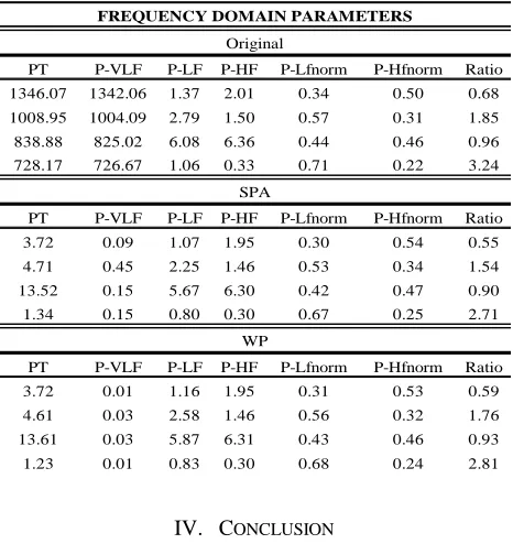
[image:5.612.61.294.363.610.2]Table II. Effect of detrending techniques on the frequency domain
parameters. Total power (PT) (ms2), Very Low Frequency power (P-VLF) (ms2
), Low Frequency power (P-LF) (ms2
), High Frequency power (P-HF) (ms2
), Normalized Low Frequency power (P-Lfnorm) (n.u), Normalized High Frequency power (nu) and
Ratio (P-LF/P-HF)
PT P-VLF P-LF P-HF P-Lfnorm P-Hfnorm Ratio
1346.07 1342.06 1.37 2.01 0.34 0.50 0.68
1008.95 1004.09 2.79 1.50 0.57 0.31 1.85
838.88 825.02 6.08 6.36 0.44 0.46 0.96
728.17 726.67 1.06 0.33 0.71 0.22 3.24
PT P-VLF P-LF P-HF P-Lfnorm P-Hfnorm Ratio
3.72 0.09 1.07 1.95 0.30 0.54 0.55
4.71 0.45 2.25 1.46 0.53 0.34 1.54
13.52 0.15 5.67 6.30 0.42 0.47 0.90
1.34 0.15 0.80 0.30 0.67 0.25 2.71
PT P-VLF P-LF P-HF P-Lfnorm P-Hfnorm Ratio
3.72 0.01 1.16 1.95 0.31 0.53 0.59
4.61 0.03 2.58 1.46 0.56 0.32 1.76
13.61 0.03 5.87 6.31 0.43 0.46 0.93
1.23 0.01 0.83 0.30 0.68 0.24 2.81
FREQUENCY DOMAIN PARAMETERS
Original
SPA
WP
IV. CONCLUSION
In this study the performance of two different methods one based on SPA and another using WP analysis was evaluated using simulated and real RR-interval time series. Both these methods seem to have satisfactorily removed the slow varying trend from the real RR-interval (see Fig. 5 and Fig. 9).
Results shown in Fig. 4 and Fig. 8 highlight the importance of the use of simulated signals with known characteristics in evaluating these kinds of algorithms. The spectrum shown in Fig. 4(c) which is obtained by detrending
the simulated signal 1, using the SPA, indicates that the slow varying signal component has been attenuated to a value of approximately 0.3 from a value of 1. The detrending filter has also caused some reduction in the power of the second component of the signal, which in this case is reduced to about 0.8 (Fig. 4(c)). From the results shown in Fig. 3(b) and Fig. 4(d) it can be seen that in the case of the second simulated signal the trend is not removed properly. Also, due to the slow transition of the filter from the stopband to the passband the LF component of the signals are getting attenuated as well (Fig. 4(c) and Fig. 4(d)). Compare to this, the detrending algorithm based on the WP analysis achieved much better results, as it offer more attenuation of the slow varying trend without causing reduction in the other regions of the signal (Fig. 7 and Fig. 8). The better performance achieved by the WP method in the case of real RR-interval time series can be seen by comparing the spectrums shown in the top row of Fig. 10 with those shown in the top row of Fig. 6. These results indicate that in the case of real RR-interval time series the LF component of the signal is slightly better preserved in the case of the WP detrended signal as compared to the signal obtained after SPA detrending. Similar conclusion can be drawn from the values shown for different time domain and frequency domain parameters presented in table I and table II respectively. From the indices shown in table I it can be seen that both the detrending techniques have affected SDNN, which describes the total variance of the signal, the most. For the other two indices (RMSSD and pNN50) the values obtained after WP detrending are slightly better matched with the original values than the ones obtained by SPA detrending method. Lastly, processing capability and speed of the two algorithms should also be considered. The SPA is simple to implement but it requires more computation time and also can not handle a large data set.
REFERENCES
[1] T. F. of the Euro. Society of Cardiology the N. American Society of
Pacing Electrophysiology, “Heart Rate Variability Standards of Measurement, Physiological Interpretation, and Clinical Use,”
European Heart Journal, vol. 17, pp. 354-381, 1996.
[2] D. Litvack, T. Oberlandern, L. Carney, and J. Sau, “Time and
frequency domain methods for heart rate variability analysis: A methodological comparison,” Psychophysiol., vol. 32, pp. 492–504, 1995.
[3] I. Mitov, “A method for assessment and processing of biomedical
signals containing trend and periodic components,” Med. Eng. Phys., vol. 20, pp. 660–668, 1998.
[4] S. Porges and R. Bohrer, The analysis of periodic processes in
psychophysiological research,” Principles of Psychophysiology
Physical Social and Inferential Elements (J. Cacioppo and L.
Tassinary, eds.), pp. 708-753, Cambridge University Press, 1990.
[5] P. M. Tarvainen, O. P. Ranta-aho, and P. A. Karjalainen, “An
advanced detrending method with application to HRV analysis,”
IEEE Trans. Biomed. Eng., vol. 49(2), pp. 172–175, 2002.
[6] R. D. Berger, S. Akselrod, D. Gordon, and R. Cohen, “An efficient