An Examination into the Structure of Freight Rates in the Shipping Freight Markets

(1)

City, University of London Institutional Repository

Citation

:

van Dellen, S. (2011). An Examination into the Structure of Freight Rates in the Shipping Freight Markets. (Unpublished Doctoral thesis, City University London)

This is the accepted version of the paper.

This version of the publication may differ from the final published

version.

Permanent repository link: http://openaccess.city.ac.uk/7789/

Link to published version

:

Copyright and reuse:

City Research Online aims to make research

outputs of City, University of London available to a wider audience.

Copyright and Moral Rights remain with the author(s) and/or copyright

holders. URLs from City Research Online may be freely distributed and

linked to.

(2)

An Examination into the Structure of Freight

Rates in the Shipping Freight Markets

Stefan van Dellen

Supervisors:

Professor Nikos K. Nomikos

Dr. Amir H. Alizadeh

A thesis submitted for the degree of Doctor of Philosophy

(3)

(4)

Table of Figures

Figure 1.1 – The Demand Function for Bulk-Shipping Services ... 26

Figure 1.2 – The Supply Function for Bulk-Shipping Services... 28

Figure 1.3 – The Short-Run Market Equilibrium for Bulk Shipping Services ... 29

Figure 1.4 – Dry-Bulk Sector Market Cycles from 1741 to 2007 ... 32

Figure 1.5 – Evolution of Tanker Spot Freight Rates Between 13 January 1989 and 26 June 2009 ... 34

Figure 1.6– Evolution of Dry-Bulk Spot Freight Rates Between 13 January 1989 and 26 June 2009 ... 35

Figure 1.7 – Cumulative Impulse Response Functions ... 42

Figure 4.1 – Evolution of Tanker Spot Freight Rates (13 January 1989 to 26 June 2009) ... 160

Figure 4.2 – Evolution of Dry-Bulk Spot Freight Rates (13 January 1989 to 26 June 2009) ... 161

Figure 4.3 – Tanker Freight Rate Returns (13 January 1989 to 26 June 2009) ... 167

Figure 4.4 – Dry-Bulk Freight Rate Returns (13 January 1989 to 26 June 2009) ... 168

Figure 4.5 – Distribution of VLCC Returns vs. Normal Distribution ... 170

Figure 4.6 – Distribution of SZMX Returns vs. Normal Distribution ... 170

Figure 4.7 – Distribution of AFMX Returns vs. Normal Distribution ... 171

Figure 4.8 – Distribution of CPSZ Returns vs. Normal Distribution ... 171

Figure 4.9 – Distribution of PNMX Returns vs. Normal Distribution ... 172

Figure 6.1 – Conditional Annualised Volatility for the GARCH Models ... 206

Figure 6.2 – Conditional Annualised Volatility for the IGARCH Models ... 209

Figure 6.3 – Conditional Annualised Volatility for the FIGARCH Models ... 213

Figure 7.1 – Conditional Moments for GARCHSK Model of the VLCC Series ... 232

Figure 7.2 – Conditional Moments for GARCHSK Model of the SZMX Series ... 232

Figure 7.3 – Conditional Moments for GARCHSK Model of the AFMX Series ... 233

Figure 7.4 – Conditional Moments for GARCHSK Model of the CPSZ Series ... 233

(9)

(10)

List of Tables

Table 1.1 – Classification of Dry-Bulk Vessels... 22

Table 1.2 – Classification of Tanker Vessels... 23

Table 4.1 – Descriptive Statistics for Spot Freight Rates and Returns ... 164

Table 4.2- Unit Root Test for Spot Freight Rate Levels and First-Differences ... 165

Table 4.3 – Ljung-Box Tests for the Freight Rate Series ... 174

Table 5.1 – Results for Unit Root Tests of Spot Freight Rate Levels ... 183

Table 5.2 – Results for Final ARMA Models of Spot Freight Rate Levels... 184

Table 5.3 – Results for Final ARIMA Models of Spot Freight Rate Levels ... 185

Table 5.4 – Results for ARFIMA (0; d; 0) Models of Spot Freight Rates ... 186

Table 5.5 – Results for Nielsen (2005) Tests on Residuals of ARFIMA Models ... 188

Table 5.6 – Results for ARFIMA (p; d; q) Models of Spot Freight Rates ... 189

Table 5.7 – In-Sample Model Comparison Results ... 191

Table 5.8 – Comparison of Forecasting Performance ... 193

Table 6.1 – ARFIMA-GARCH Model Results ... 204

Table 6.2 – ARFIMA-GARCH Standardised Residual Diagnostics ... 207

Table 6.3 – ARFIMA-IGARCH Model Results ... 208

Table 6.4 – ARFIMA-IGARCH Standardised Residual Diagnostics ... 210

Table 6.5 – ARFIMA-FIGARCH Model Results ... 212

Table 6.6 – ARFIMA-FIGARCH Standardised Residual Diagnostics ... 214

Table 6.7 – Results for the Model Selection Criteria... 217

Table 7.1 – Empirical Results for the ARFIMA-GARCHSK Model ... 229

Table 7.2 – Residual Diagnostics for the ARFIMA-GARCHSK Model... 235

Table 7.3 – Conditional Variance Statistics for the ARFIMA-GARCH Model ... 237

Table 7.4 – Conditional Variance Statistics for the ARFIMA-FIGARCH Model .... 237

Table 7.5 – Conditional Variance Statistics for the ARFIMA-GARCHSK Model ... 237

Table 7.6 – Likelihood-Ratio Test Results for Comparison of Models ... 239

Table 8.1 – Value-at-Risk Results on a Long Position for the VLCC Data Series ... 256

Table 8.2 – Value-at-Risk Results on a Long Position for the SZMX Data Series ... 257

Table 8.3 – Value-at-Risk Results on a Long Position for the AFMX Data Series .. 259

Table 8.4 – Value-at-Risk Results on a Long Position for the CPSZ Data Series .... 260

Table 8.5 – Value-at-Risk Results on a Long Position for the PNMX Data Series .. 262

Table 8.6 – Value-at-Risk Results on a Short Position for the VLCC Data Series ... 264

Table 8.7 – Value-at-Risk Results on a Short Position for the SZMX Data Series ... 265

Table 8.8 – Value-at-Risk Results on a Short Position for the AFMX Data Series .. 266

Table 8.9 – Value-at-Risk Results on a Short Position for the CPSZ Data Series .... 267

(11)

(12)

List of Abbreviations

$ / Day US$ per Day

ADF Augmented Dickey-Fuller Unit Root Test

AFMX Aframax Vessel

AIC Akaike Information Criterion

AR Autoregressive

ARCH Autoregressive Conditional Heteroscedasticity

ARFIMA Autoregressive Fractionally Integrated Moving Average Model

ARIMA Autoregressive Integrated Moving Average Model

ARMA Autoregressive Moving Average Model

BIFFEX Baltic International Freight Futures Exchange

CC Conditional Coverage Test

CDIR Percentage of Correct Direction Predicted

CF Cornish-Fisher Expansion

( )

;

CI x y Cointegrated of Order x and y

CPSZ Capesize Vessel

D Level of Demand

d Order of Fractional Integration

DWT Dead-Weight Tonnes

EGARCH Exponential Generalised Autoregressive Conditional

Heteroscedasticity Model

ES Expected Shortfall

ESTAR Exponentially Smooth Transition Autoregression Model

EWMA Exponentially Weighted Moving Average

FFA Forward Freight Agreement

FHS Filtered Historical Simulation

FHS (200) Filtered Historical Simulation over a 200 Week Horizon

FHS (400) Filtered Historical Simulation over a 400 Week Horizon

FIEGARCH Fractionally Integrated Exponential Generalised Autoregressive

Conditional Heteroscedasticity Model

FIGARCH Fractionally Integrated Generalised Autoregressive Conditional

GARCH Generalised Autoregressive Conditional Heteroscedasticity

Model

GARCHK Generalised Autoregressive Conditional Heteroscedasticity and

Kurtosis Model

GARCHS Generalised Autoregressive Conditional Heteroscedasticity with

Skewness Model

GARCHSK Generalised Autoregressive Conditional Heteroscedasticity with

Skewness and Kurtosis Model

GARCH-X Augmented Generalised Autoregressive Conditional

GC Gram-Charlier Expansion

HS Historical Simulation

HS (200) Historical Simulation over a 200 Week Horizon

(13)

( )

I x Integrated of Order x

IGARCH Integrated Exponential Generalised Autoregressive Conditional

Ind Independence Test

KPSS Kwiatkowski, Phillips, Schmidt and Shin Unit Root Test

KSS Kapetanios, Shin and Snell Unit Root Test

LF Loss Function

LL Log-Likelihood

LM Lagrange-Multiplier Test

LR Likelihood-Ratio Test

MA Moving Average

MAE Mean Absolute Error

MAPE Mean Absolute Percentage Error

MDM Modified Diebold-Mariano Test

MLE Maximum Likelihood Estimation

NAGARCHSK

Non-Linear Asymmetric Generalised Autoregressive Conditional Heteroscedasticity with Skewness and Kurtosis Model

OLS Ordinary Least Squares Estimation

PNMX Panamax Vessel

QMLE Quasi-Maximum Likelihood Estimation

RM RiskMetricsTM Model

RMSE Root Mean Squared Error

S Level of Supply

SBIC Schwartz-Bayesian Information Criterion

SGT Skewed Generalised t-Distribution

SZMX Suezmax Vessel

TCE Time-Charter Equivalent Freight Rate

UC Unconditional Coverage Test

ULCC Ultra-Large Crude Carrier Vessel

VaR Value-at-Risk

VAR Vector Autoregressive Model

VECM Vector Error Correction Model

VLCC Very Large Crude Carrier Vessel

(14)

Dedication

(15)

(16)

Acknowledgements

Although it is not possible to specifically name everyone who has helped me during

the various stages of this thesis and my research studies, I would like to express my

greatest thanks and sincere appreciation to my two supervisors Dr. Nikos Nomikos

and Dr. Amir Alizadeh for their support, patience and everlasting encouragement

throughout these years. Furthermore, I would like to thank my thesis examiners Prof.

Roy Batchelor and Dr. Dong-Wook Song for their invaluable feedback and guidance.

I am also grateful to Prof. Costas Grammenos for his help throughout my time at Cass

and would also like to remember the support of the late Prof. Anthony Lumby. I wish

to thank Malla Pratt and Abdul Momin for all their invaluable help, as well as my

fellow PhD students at Cass, whom I will not refer to by name for fear of leaving

anyone out, for being there through all the good as well as the bad times and

providing a listening ear. I would finally like to thank my parents, James and Doria

van Dellen, as well as my brothers, Anton, David and Jonathan, and other members of

(17)

Declaration

I grant the powers of discretion to the City University Librarian to allow this thesis to

be copied in whole or in part without further reference to me. This permission covers

only single copies made for educational purposes, subject to normal conditions of

(18)

Abstract

This thesis investigates three salient areas of interest in the structure of freight rates in

the shipping market, with a particular focus on the tanker and dry-bulk sectors, using

recent econometric and time series techniques. The questions asked are: 1) do spot

freight rate levels follow a fractionally integrated process, as opposed to being

stationary or non-stationary, as had previously been proposed; 2) does spot freight

rate volatility also follow a fractionally integrated process; and 3) do freight rates

exhibit conditional skewness and kurtosis? It then evaluates the impact that these

factors have on the risk exposure of market participants. These concepts are further

tested in terms of their respective forecasting performance, relative to other more

standard econometric techniques.

An ongoing issue in the shipping literature is whether spot freight rate levels follow a

stationary or non-stationary process. This thesis provides another dimension to this

discussion by arguing that spot freight rate levels follow a fractionally integrated

process. The rationale behind this argument is the fact that the supply and demand

dynamics in this market mean that although freight rates are mean-reverting overall,

the process of mean-reversion occurs with a delay, which is exactly how one would

expect a fractionally integrated process to behave. Although in-sample results were

promising in that fractionally integrated models are found to outperform their

stationary and non-stationary counterparts across sectors and vessel sizes,

out-of-sample forecasts indicate that models that assumed stationarity or

non-stationarity outperformed these models, depending on the sector and vessel size.

Additionally, the thesis extends this debate to the volatility of these spot freight rate

levels, where it is proposed that volatility also follows a fractionally integrated

process. In-sample results from the estimation of Generalised Autoregressive

Conditional Heteroscedasticity (GARCH), Integrated Generalised Autoregressive

Conditional Heteroscedasticity (IGARCH) and Fractionally Integrated Generalised

Autoregressive Conditional Heteroscedasticity (FIGARCH) models indicate that

FIGARCH models outperformed the other two models across all sectors and vessel

(19)

vessel type, non-parametric models are found, in most cases, to outperform their

parametric counterparts across sectors and vessel sizes.

This thesis finally examines whether freight rates exhibit conditional skewness and

kurtosis, where the shape of the supply function in the shipping freight markets

indicates that these would not be constant over time, as is assumed by other standard

models. Results for the in-sample period indicate that the Generalised Autoregressive

Conditional Heteroscedasticity with Skewness and Kurtosis (GARCHSK) models

outperformed GARCH and FIGARCH models. This being said, when calculating the

respective out-of-sample Values-at-Risk for each vessel type, non-parametric models

are found, in most cases, to outperform their parametric counterparts across

(20)

1 Review of the Shipping Market and Hypotheses

1.1 General Introduction

For almost as long as people have been trading goods, the primary means of

transportation for these goods has been by ship, thus demonstrating the enduring

importance of the shipping industry to the world economy as a whole. To illustrate

this point, it was estimated that seaborne trade in 2007 was over 7,500 million tonnes,

with the demand for shipping services equating to over 32,900 billion tonne-miles.1

For this reason, from when they were first discussed by Koopmans (1939), freight

rates, or the price of transporting goods by sea, have been a constant source of

practical and academic interest.

The academic interest has primarily been focused on modelling the freight rates, but

an ongoing debate as to the degree of stationarity, and therefore the correct models to

use, has continued for almost twenty years since the advent of unit root tests. Within

this debate, general and partial equilibrium models, for example those proposed by

Beenstock and Vergottis (1989) and Koekebakker, et al. (2006), amongst others,

argue that the first moment of freight rates, i.e. spot freight rate levels, are stationary.

The contrasting view, as outlined in such papers as Berg-Andreassen (1997) and

Kavussanos and Visvikis (2004), amongst others, proposes that unit root tests indicate

that these spot freight rates are in fact non-stationary. The debate extends to the issue

of the structure of volatility, or second moment, of these freight rates where

Kavussanos (1997) argues that volatility exhibits persistence, while Kavussanos and

Nomikos (2003) are happy to assume that there is no persistence in volatility. This

thesis adds a new dimension and middle ground to the debate by suggesting that both

the first and second moments of freight rates are fractionally integrated where, to the

best of the author’s knowledge, this is done for the first time in the shipping literature.

In addition, this thesis examines, where once again, the author is unaware of previous

research on this topic in the shipping literature, the third and fourth moments of

1

(21)

freight rates, and in particular, introduces the concept of conditional skewness and

kurtosis to the shipping academic literature.

An interesting point to highlight is that the shipping market is, perhaps, one of the few

markets in which the underlying good provided is a service, and hence intangible.

This being said, it is worth considering that these methodologies are not market

specific; already a significant amount of interest in fractionally integrated models

exists in other markets, see for example Baillie, et al. (1996b) and Kang, et al. (2009),

amongst many others. In addition, this methodology can be readily applied to other

markets, such as the real estate market, in which real assets are traded.

In summary, this thesis aims to give an insight into the structure of freight rates,

through the examination of the various moments in these series. A thorough, and

correct, understanding of the structure is of great interest as freight rates play a pivotal

role and form the basis of almost every function in the shipping industry, from

the determination of the price of the transport service through to the valuation of

second-hand vessels. For this reason a correct model for freight rates is vital for all

participants in the market, from the ship-owners and charterers themselves, right on

down through the market to ship-brokers, maritime lawyers, hedge funds and other

auxiliary parties involved. To give a structure to this concept, this chapter begins by

reviewing the structure of the underlying shipping market, before moving on to

outline the four main hypotheses that form the basis of the thesis.

1.2 Review of the Shipping Market

The shipping industry can be divided into several segments, such as, those for tanker,

dry-bulk, container, reefer and cruise vessel vessels; however, a more general

approach, commonly taken, is to divide the shipping market into two main

sub-markets, namely the liner and bulk-shipping markets. Liner shipping is generally

characterised by vessels that operate along pre-specified, fixed routes according to a

regular, fixed schedule, where the majority of these vessels are now container ships.

Essentially, what characterises the liner sector as distinct from the bulk sector is the

(22)

loaded onto the vessel, and ends when they are offloaded onto the quayside. The

freight rates in the liner sector are consequently generally fixed and there is usually

very little negotiation between parties with respect to these. Bulk-shipping, on the

other hand, is different in that the vessels in this sector usually operate when and

where the charterer demands them. Additionally, freight rates in the bulk sector vary

widely and are a matter of negotiation between the ship-owner, and are therefore

mostly negotiated privately. Focusing on the bulk-shipping sector, this can be further

sub-divided into the dry-bulk and tanker sectors, where this classification depends on

the characteristics of the cargo that the vessel will carry. In general, dry-bulk vessels

will carry dry cargo, such as coal, grain or iron ore, while tankers generally carry

liquid cargo, such as crude oil or oil products, although combined carriers do exist

which may operate in both markets, even though these are no longer in vogue.

As a result of the historic stability of freight rates in the liner industry, the consequent

lack of volatility renders asset play and freight modelling strategies unnecessary and

therefore costly, and provides little scope for interest from auxiliary parties, such as

hedge funds. To illustrate this point, Clarksons Research Services Ltd. (2010) show

that there were only 123 container vessels sold, totalling 2.6 million DWT and worth

US$742 million, during 2009, as opposed to 153 tanker vessels, totalling 14.9 million

DWT and worth US$3,674 million, and 584 dry-bulk vessels, totalling 32.2 million

DWT and worth US$8,846 million, during the same period.2 In addition to this, the

vast majority of vessels lie within the bulk-shipping sector, where for example, ISL

Bremen (2008) indicates that, in 2007, 77% of the world seaborne fleet was

comprised of either dry-bulk or tanker vessels.3 Consequently, this research will focus

exclusively on the bulk-shipping sector of the shipping market; and, hence, on the

freight rates exhibited in the dry-bulk and tanker sectors of the shipping market.

Given this fact, however, it is very interesting to note that the freight rates in the liner

sector have become much more volatile recently, mostly as a result of the credit crisis;

therefore the methodologies and hypotheses outlined in this thesis may be applied to

this sector as a future potential extension of the work considered here.

2_{This disparity is further illustrated in Figures A01 to A03, in Appendix A of the thesis.} 3

(23)

1.2.1 The Dry-Bulk and Tanker Sectors

As mentioned above, the bulk-shipping sector is commonly sub-divided into the

dry-bulk and tanker sectors. The two sectors share a number of common

characteristics, the first of which is that, in both sectors, the commodities carried tend

to be low-value products, hence their suitability for slow, cheap transportation in large

consignments, where this is to achieve economies of scale. One reason for this is that

the costs of alternative means of transportation, such as transporting these goods by

air or container, is prohibitive, in addition to the fact that these goods are generally

transported in such large consignments as to make other means of transport

unfeasible. The second common characteristic is that these sectors constitute the

majority of seaborne trade; where, for example, ISL Bremen (2008) illustrate that of

the 7,572 million tonnes of cargo transported by sea, at least 58% of this was either

dry- or liquid-bulk cargo.4 The final common characteristic is that the size of the

vessels, in both sectors, is measured in dead-weight tonnes (DWT), as opposed to the

container sector, where ship size is generally measured in terms of the number of

twenty foot containers they can carry. Stopford (2009) defines the DWT as the

maximum amount of cargo, in terms of weight, that a vessel can carry, without being

classified as overloaded. One should note that this measure includes the weight of any

fuel, stores, water ballast, fresh water, passengers and baggage. Having established

these three characteristics, one can now proceed to individually examine

[image:23.595.91.511.558.636.2]

characteristics of each market.

Table 1.1 – Classification of Dry-Bulk Vessels

Vessel Class Size (DWT)

Capesize Dry-Bulk Vessels Over 80,000

Panamax Dry-Bulk Vessels 60,000 to 79,999

Handymax Dry-Bulk Vessels 40,000 to 59,999

Handysize Dry-Bulk Vessels 10,000 to 39,999

Source: Clarksons Research Services Ltd. (2010)

Beginning with the dry-bulk sector, ISL Bremen (2008) show that, although only 16%

of the world fleet in 2007, in terms of vessels, was comprised of dry-bulk vessels, this

sector comprised 35% of the cargo carrying capacity, and 26% of world trade, in

4

(24)

terms of all cargo carried. Of these commodities carried, the predominant cargoes are

iron ore, coal and grain, commonly known as the major bulks, where in 2007 trade of

these exceeded 1.9 billion tonnes, and where, as mentioned above, this was equal to

the 26% of the total world trade by sea.5 The size of dry-bulk vessels can range from

small coastal vessels, of less than 1,000 DWT, to huge Capesize vessels of over

300,000 DWT. The major classifications of these vessels are provided in Table 1.1.

The dry-bulk trade has grown steadily over the years (particularly with the

development of China and India as major economic powers) where this has been

fuelled by world economic growth and the consequent demand for bulk commodities,

such as coal and iron ore.6 This growth is not immune to current economic conditions,

and with the current recessions, levels of trade have fallen, although the markets

appear to have picked up somewhat recently. An indication of this is that annual

weighted average earnings, i.e. earnings weighted for the size of vessels, as reported

by Clarksons Research Services Ltd. (2010), fell from a high of US$43,649 per day in

2007 to US$15,016 per day in 2009, although these have recovered to US$21,677 per

[image:24.595.84.506.464.568.2]

day, for the year to date in 2010.7

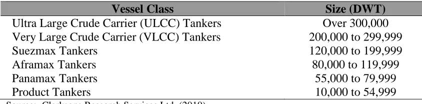
Table 1.2 – Classification of Tanker Vessels

Vessel Class Size (DWT)

Ultra Large Crude Carrier (ULCC) Tankers Over 300,000

Very Large Crude Carrier (VLCC) Tankers 200,000 to 299,999

Suezmax Tankers 120,000 to 199,999

Aframax Tankers 80,000 to 119,999

Panamax Tankers 55,000 to 79,999

Product Tankers 10,000 to 54,999

Source: Clarksons Research Services Ltd. (2010)

Changing the focus to the tanker sector, the predominant cargoes here are either crude

oil, generally carried by larger tankers, or refined oil products, such as heating oil, jet

fuel, liquefied natural gas, to name but a few. As with the dry-bulk sector, when

looking at the figures from ISL Bremen (2008), the fact tankers comprise only 25% of

5

A graphical breakdown of the composition of trade in the three major dry-bulk commodities, by commodity, can be found in Figure A07, in Appendix A of the thesis.

6_{This is illustrated in Figure A08, in Appendix A of thesis, which shows the evolution of dry-bulk} trade against world trade for the ten year period between 1988 and 2007.

7

(25)

the world fleet, in terms of the number of vessels, severely under-represents the

importance of the sector as it comprises 41% of the world fleet, in terms of cargo

carrying capacity. Moreover, trade in liquid-bulk cargoes comprised 32%, or 2.4

billion tonnes, of the total world trade of 7.6 billion tonnes.8 The size of tankers

ranges from small barges, used to transport bunkers, to the enormous Ultra Large

Crude Carriers (ULCCs), which can range up to 550,000 DWT. The classification of

tankers is summarised in Table 1.2. For the purposes of this study, the ULCC and

Very Large Crude Carrier (VLCC) markets have been combined for ease.

As with the dry-bulk sector, the tanker sector has grown steadily over the years as

world economic growth and increased demand for crude oil and oil products has

increased the demand for transportation.9 However, the tanker sector is, as stated

above, also not immune to current economic conditions, and, with the advent of the

latest recession, tanker rates plummeted. To illustrate this point, average annual

weighted earnings for tankers, as reported by Clarksons Research Services Ltd.

(2010), fell from US$44,130 per day in 2008 to $15,511 per day in 2009; however,

the market has shown signs of recovery in 2010, to date, with average weighted

earnings of $21,583 per day.10

A further small point to note regarding the dry-bulk and tanker sectors is the manner

in which freight rates are quoted differs across sectors. In the tanker sector, freight

rates are quoted in terms of the Worldscale (WS), which can then be converted into

US$ per tonne, according to the route, using the Worldscale Book, which is revised

annually. In contrast, dry-bulk sector freight rates are simple quoted in terms of US$

per tonne, regardless of the route on which the goods are transported.

Having established the characteristics of each of sector, one can now move on to

explore the underlying characteristics, in terms of supply and demand, for the

shipping market as a whole, and how these play a role in determining freight rates.

8

A graphical breakdown of the composition of tanker trade, by commodity, can be found in Figure A10, in Appendix A of the thesis.

9_{This is illustrated in Figure A11, in Appendix A of thesis, which shows the evolution of tanker trade} against world trade for the ten year period between 1988 and 2007.

10

(26)

1.2.2 The Demand for and Supply of Bulk-Shipping Services

Having examined the structure of the individual sectors of the shipping market, one

can now move on to examine what factors drive the bulk-shipping sector, i.e. the

determinants of the demand and supply functions, both of which determine the level

of freight rates in the market.

Since the demand for bulk-shipping services is a demand for the transportation of

goods, this demand is derived from the demand for the goods being carried and is

therefore susceptible to the cyclical nature of world trade. However, although this is a

derived demand, Stopford (2009) illustrates that it can be divided into five main

determinants, namely: 1) the level of world economic activity; 2) the level of seaborne

commodity trade; 3) the average haul, or, in other words, the distance over which the

commodities must be carried; 4) current political events; and, finally, 5) the level of

transportation costs.

If the level of world economic activity is high, there will, of course, be a high demand

for commodities, and, consequently, a high demand for the means with which one

would transport these, hence, the demand for bulk-shipping services will increase.

Moreover, even if the above does not hold, if the level of seaborne commodity trade is

high, then the demand for shipping will naturally increase, due to the nature of the

service provided. Another factor that would increase the demand for vessels in the

bulk sector would be if the average haul were to increase, for example, if new oil

fields were discovered in a remote part of the world. The reason for this is that

charterers would seek to take advantage of the economies of scale offered by

bulk-shipping to drive down their transportation costs, as well as the fact that fewer vessels

would be available for hire. Looking at the fourth factor, political events can either

have a positive or negative effect on the demand for bulk-shipping, depending on

whether the news is perceived as good or bad. An example of how good news for the

bulk-shipping industry would impact on demand for their services was when the Suez

Canal was closed during the 1970s, where tankers transporting oil from the Middle

East to Europe and the US East Coast were forced to round the Cape of Good Hope,

thus resulting in increased average hauls. However, on the negative side, the

(27)

[image:27.595.124.474.99.452.2]

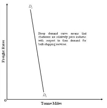
Figure 1.1 – The Demand Function for Bulk-Shipping Services

liable under certain cases for clean-up costs in the event of a spill, meant that

charterers looked for other alternatives, such as overland pipelines, to transport their

cargoes, thereby reducing the demand for shipping as a means of transport. The final

factor is that if transport costs are high, then bulk-shipping may become attractive to

charterers as they seek to take advantage of the economies of scale provided, thereby

increasing the demand for their services.

Looking at the demand function in Figure 1.1, one should note that the demand

function is relatively price inelastic, i.e. demand for bulk-shipping services will only

decrease by a very small amount, for a fixed increase in the freight rates. A reason for

this is that, on the whole, the cost of transportation is only a very small part of the

overall cost of the product, therefore, although charterers are still sensitive to price

changes, they are much less sensitive than they would be, for example, with respect to

(28)

charterer, and therefore it is a case of necessity to pay whatever is demanded to be

able to transport the commodities.

As mentioned above, ISL Bremen (2008) show that, in 2007, over 7.5 billion tonnes

of cargo were transported by sea, and these were transported over 4,439 billion

nautical miles, corresponding to a demand for shipping of 22,018 billion tonne-miles.

Of this demand, 12,440 billion tonne-miles, or 38% of the total, corresponded to the

dry-bulk sector, and 10,397 billion tonne-miles, or 32% of the total, to the tanker

sector, thus serving to reinforce the importance of both these sectors.

Changing focus to the supply-side of the market, Stopford (2009) argues that the

supply of shipping services depends on five major factors, namely: 1) the fleet stock,

i.e. the number of vessels operating; 2) ship-building production, i.e. the number of

new vessels being built; 3) scrapping, i.e. the number of vessels scrapped for scrap

metal, and losses, or vessels lost at sea or damaged beyond repair; 4) fleet

productivity; and 5) the current level of freight rates in the market. Furthermore, one

should also note that the supply of shipping is fixed in the short-term, for

reasons discussed below.

Beginning with the fleet stock, it is fairly obvious that the higher the fleet stock, the

greater the supply of bulk-shipping in that there are more vessels available to carry

goods. Clarksons Research Services Ltd. (2010) reports that, as of May 2010, there

are 7,541 dry-bulk vessels, totalling 481 million DWT, and 5,353 tankers, totalling

442 million DWT, meaning that the bulk-shipping fleet is at its highest levels for at

least forty years. Moving on to ship-building production - as new vessels enter the

market, so supply increases and Clarksons Research Services Ltd. (2010) report that,

during 2009, 544 dry-bulk vessels and 580 tankers were delivered, corresponding to

43 and 48 million DWT, respectively, once again the highest figures for over 40

years. As far as scrapping and losses are concerned, an increase in these would lead to

a corresponding decrease in the supply of bulk-shipping. Scrapping levels are

relatively low at the moment, but increasing, while the current market conditions, in

terms of the low freight rates, mean that a lot of the fleet is slow-steaming, i.e. not

operating a the maximum speed possible, thereby further reducing the supply of

(29)

[image:29.595.127.452.122.445.2]

Figure 1.2 – The Supply Function for Bulk-Shipping Services

new-buildings being delivered mean that the supply of bulk-shipping is at record

levels, and, given the current state of the order-book for new vessels, is likely to keep

growing. This is not an ideal position for the bulk-shipping to be in, considering that

the world is currently only just recovering from one of the worst recessions since the

Great Depression, and where shipping is merely a means of transport for

this world trade.

The shape of the supply function, illustrated in Figure 1.2, can be explained by the

fact that supply is fixed in the short-term. The reason for this is that it can take up to

three years, sometimes even longer, for a vessel to be delivered, i.e. from the time the

vessel is ordered to when the ship-owner takes possession. This means that, with the

exception of scrapping vessels or placing vessels in lay-up, when freight rates are so

(30)

[image:30.595.118.480.108.444.2]

Figure 1.3 – The Short-Run Market Equilibrium for Bulk Shipping Services

relatively fixed, at S until the new-buildings are delivered, where the supply ₁

function in Figure 1.2 will shift outwards from S to ₁ S . However, one should note 2

that even delivering vessels for scrapping may take a few months; hence this may also

delay any adjustments to the supply function.

Having established the characteristics of the supply and demand functions for

bulk-shipping, one can now move on to examine the mechanics of the freight rate

mechanism and the impact that this has on volatility in the shipping markets.

1.2.3 Freight Rates and Volatility in the Bulk-Shipping Sectors

The prevailing freight rate, which is the name for the prices of the transport service,

are determined from the interaction between the supply and demand functions,

(31)

Figure 1.3. If we remember that the supply function is fixed in the short-run, then, as

the demand function shifts along this fixed supply function, the prevailing freight

rates will change accordingly. This means that the momentary equilibrium will

increase (decrease), if the demand for the bulk-shipping services increases (decreases)

accordingly, with the magnitude of the change in price depending on the price

elasticity of the supply function at the point of equilibrium. Using the example given

in Figure 1.3, if one begins at Point A, a 50% increase in demand, from D to ₁ D , ₂

will result in a small increase in freight rates, from FR to ₁ FR , corresponding to 2

Point B, while a 10% further increase in demand, from D to 2 D , would result in a 3

much bigger increase in freight rates, from FR to ₂ FR , corresponding to Point C. ₃

The reason for this discrepancy is that the price elasticity of the supply function at

Point B is much lower than at Point C, as there is still excess capacity in terms of

supply, whereas at Point C, supply is pretty much at the maximum short-term level.

In the long-run, the supply function may shift either inwards, if the level of scrapping

exceeds the level of new-building deliveries, or outwards, if the reverse applies. This

ratio of scrapping vessels to new-building orders will depend on market sentiments

about the future direction of freight rates. If market sentiments are good, which would

correspond to ship-owners feeling that freight rates are likely to remain high or

increase in the future, then the supply function may shift to the right, as the

ship-owner delays any scrapping activity and places orders for new vessels to benefit from

the boom. The reverse would apply when ship-owners felt that freight rates are

depressed, or are likely to fall in the future, as happened last year, in which case

ship-owners would seek to scrap unprofitable vessels and delay any orders. Over time, as

the long-run supply of ships adjusts from a previous under- or over-supply of tonnage,

freight rates will revert to the mean level that existed prior to the observable changes

in the supply function.

Moving to look at the volatility of shipping freight rates, or the risk inherent in the

market, one should be aware that the shipping industry is highly dependent on a

number of external factors, over which market agents have no control. This means

(32)

this size-volatility relationship is that smaller ships are more versatile in terms of the

cargo they can carry and ports they can visit, hence they can operate in multiple

markets. In contrast, a larger vessel is limited in terms of the cargo it can carry, due to

the size of the cargo consignments required, and ports it can visit, as a result of draft

constraints. Another reason for this volatility is the volatile nature of the demand for

the goods being carried. For example, it is common knowledge that the demand for

crude oil and refined oil products increases during the Northern Hemisphere winter,

due to the increased demand for heating, however, this demand falls dramatically in

spring. This means that the fixtures for VLCCs and other types of tankers will

increase as the Northern Hemisphere winter approaches, and falls sharply during the

spring months. In summary, all these factors cause the shipping industry to be a

highly volatile market, hence any assistance that can be given as to predicting the

nature of and relationship between factors in the industry, such as freight rates and

volatility, will be in high demand.

1.2.4 Shipping Market Cycles

No study on freight rates within the shipping market would be complete without some

comment on the market cycles within the industry. Shipping market cycles vary in

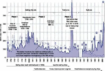
length and frequency, but it is generally accepted that there have been 22 dry-cargo

cycles between 1741 and 2007, where Figure 1.4 illustrates these cycles in the

dry-bulk sector. There are generally four stages to the shipping market cycle, namely:

the trough, the recovery, the peak, and the collapse.

During the first stage, i.e. the trough, freight rates are low, as a result of low demand.

This would mean that ships queue up at loading ports, vessels generally slow-steam to

conserve fuel and there are distress sales, i.e. sales as a result of default on loans or

due to cash shortages. The second stage, or recovery, is characterised by freight rates

beginning to increase, ships being removed from lay-up, and second-hand prices

beginning to recover as the freight market improves. Throughout the third stage, or

peak, freight rates are high, the fleet operates at full-speed, second-hand prices are

above book value, order-books are almost full, and there is no idle tonnage available,

(33)

[image:33.595.93.506.103.384.2]

Figure 1.4 – Dry-Bulk Sector Market Cycles from 1741 to 2007

Source: Stopford (2009)

occurs as a result of new orders, ordered either during the recovery or peak, being

delivered, which means that the supply of tonnage now once again exceeds demand,

hence freight rates plummet and no new orders are placed, with many ship-owners

trying to cancel existing orders.

This collapse could occur as a result of a drop in trade, due to a slowdown in the

world economy, where these effects tend to be exacerbated by negative market

sentiment. Interestingly, the shipping markets are probably coming towards the end of

the collapse stage and entering the trough phase of the cycle, where this is as a result

of the world only now beginning to recover from one of the worst recessions since the

Great Depression.

Being able to predict the future direction of freight rates, and therefore, to an extent,

the market cycles, would enable one to predict when each of the stages will occur,

thus allowing to profitably enter and exit the market, both in terms of day to day

(34)

1.2.5 A Brief Overview of the Prevailing Market Conditions

Having outlined the main characteristics of the shipping markets in general, this

subsection provides a brief overview of the prevailing market conditions in the

dry-bulk and tanker sectors in order to give context to the environment in which the

research hypotheses were formed.

Examining firstly the evolution of the tanker spot freight rates, as illustrated in

Figure 1.5, freight rates for the tanker market were relatively stable for the ten year

period up to 2001 when they experienced the first of a series of peaks which followed

over the next seven or eight years. The first peak coincides with the initiation and the

process of accelerated phasing out of single-hulled tankers in favour of the

double-hulled alternates, as a result of the amendment to the Marpol Convention. This led to

reduction in the number of vessels in the tanker fleet and a consequent decrease in the

supply of tanker services and a resultant dramatic increase in freight rates as a result

of the shape of the supply curve. The second peak corresponds to the second Gulf

War in 2003 as well as a further amendment to the Marpol Convention which

increased the scrapping schedule of single-hulled tankers, with corresponding effects

on the price of oil and supply of shipping services, and therefore freight rates. This

peak then leads on to the further peaks resulting from an increased demand for oil,

increased oil prices and the development boom in China, and therefore an increased

demand for transportation services for the oil needed. These series of peaks were

followed by an unprecedented collapse in the freight rate market in late 2008, caused

by both the world undergoing arguably the most severe economic slowdown since the

Great Depression, combined with massive over-ordering during the previous peaks

resulting in a huge number of new tankers entering the fleet thus increasing the supply

of vessels to record levels and causing an extremely and sudden fall in freight rate

levels. One could also argue that these peaks may be attributed to the rescaling of the

Worldscale rates in January, however, this is not felt to be a major factor as many of

the peaks occur in the middle of the year.

When changing focus to look at the dry bulk market, the picture is somewhat more

tranquil, as illustrated in Figure 1.6, in that freight rates remained relatively stable at

(35)

[image:35.595.85.776.157.483.2]

Figure 1.5 – Evolution of Tanker Spot Freight Rates Between 13 January 1989 and 26 June 2009

0.00 50.00 100.00 150.00 200.00 250.00 300.00 350.00 400.00 450.00

13/01/1989 13/01/1991 13/01/1993 13/01/1995 13/01/1997 13/01/1999 13/01/2001 13/01/2003 13/01/2005 13/01/2007

T im e

W

o

rl

d

s

c

a

le

(36)

[image:36.595.82.780.130.497.2]

Figure 1.6– Evolution of Dry-Bulk Spot Freight Rates Between 13 January 1989 and 26 June 2009

0.00 10.00 20.00 30.00 40.00 50.00 60.00 70.00

13/01/1989 1 3/01/1991 13/01/1993 13/01/1995 13/01/1997 13/01/1999 13/01/2001 13/01/2003 13/01/2005 13/01/2007

T im e

$

/

T

o

n

(37)

found, corresponding with increased demand for commodities driven by the growth of

the Chinese economy. The correction in the market was then followed by a massive

increase in freight around the end of 2006 and beginning of 2007, driven by a rapid

increase in the demand for commodities by China, congestion in world ports leading

to tonnage being tied up, and a dramatic increase in the price of commodities.

However, as was the case in the tanker market, a dramatic slowdown in world

economic growth, as well as over-ordering, led to as extreme a fall in freight rates,

although in this case, continued demand for commodities such as coal and iron ore, by

China led to a much faster and somewhat greater recovery.

The following section outlines the research hypotheses with the ultimate goal of

trying to achieve exactly this outcome, by understanding the structure and nature of

freight rates themselves.

1.3 Research Hypotheses

The aim of this research is to expand on the traditional models of the structure of

freight rates through the use of Autoregressive Fractionally Integrated Moving

Average (ARFIMA), Fractionally Integrated Generalised Autoregressive Conditional

Heteroscedasticity (FIGARCH) and Generalised Autoregressive Conditional

Heteroscedasticity with Skewness and Kurtosis (GARCHSK) models. Once this

has been done, these models will be used to forecast spot freight rate levels and

freight rate volatility, and then evaluate the underlying risk for market participants

through the use of the Value-at-Risk methodology. This will give one an

understanding of the behaviour of the different moments of freight rates, thereby

enabling participants in the shipping markets to have a better understanding of both

the direction of spot freight rate levels, and the underlying risk.

This research is of interest to a number of different parties, both in terms of

participants in the shipping market, as well as financial markets as a whole. One

reason for this is that it aims to add another dimension to the debate as to the exact

structure of freight rates, as well as the degree of stationarity of these, as well as

(38)

as this kind of understanding is crucial for investment timing and planning decisions,

as well as for indirectly linked parties to be able to quantify their exposure to the

market. Interestingly, the fact that the shipping freight market is perhaps one of the

few markets in which the underlying asset is a service, as well as the fact that it may

be used as a proxy for world trade, means that this market can be of interest to

participants in financial markets.

1.3.1 Background to Research Questions

As mentioned above, shipping is one of the few markets in which the good being

priced is a service, as well as being one of only a few markets in which the underlying

asset is a real asset. This research has been planned to provide critical insight into the

function of the price series within this very different type of market. Within the

shipping market, freight rates play a pivotal role in that they form the basis of almost

every function, from determining the cost of transporting goods from point A to point

B, to the valuation process for vessels themselves. Therefore, a deep understanding

and correct modelling of freight rates is essential for all participants in this market,

from the ship-owners and charterers themselves, right on down to ship-brokers,

maritime lawyers, institutional investors, such as hedge funds, and other auxiliary

parties.

Perhaps one of the most obvious uses of freight rate modelling is for decision-making

purposes, where, through the forecast of freight rates and the respective market risk,

charterers can determine when it is optimal to transport their cargo, and ship-owners

can determine where to position their vessels as well as when to enter and exit the

market. This would mean that ship-owners could maximise their earnings by

repositioning their vessels prior to the freight rate rising, and make allowances for

falling freight rates, such as re-arranging the financing of their vessels. In contrast,

while charterers could minimise their transportation costs by planning to transport as

much as possible of their goods only when market conditions are favourable.

Another, although perhaps not quite as obvious, reason for their importance is that

they allow investment timing decisions to be made. For ship-owners, as freight rates

(39)

understanding of the structure of freight rates would mean that they could determine

the ideal time to invest in new or second-hand tonnage, or either sell or scrap their

vessels. This type of asset play in the market can be crucial for risk management

purposes, due to the notoriously volatile nature of the market. An example of this is

highlighted by Clarksons Research Services Ltd. (2010), who illustrate out that

yearonyear returns from tanker earnings between 2001 and 2010 ranged from

-62.43%, in 2009, to 88.85%, in 2003. Furthermore, in the dry-bulk sector, this ranged

from -19.84%, in 2005, to 151.84% in 2010. To give an idea of the size of this

market, Clarksons Research Services Ltd. (2010) show that at the peak of the market,

in 2007, trade in second-hand vessels was worth US$47.8 billion, consisting of 1,873

individual transactions and 85.6 million DWT. For institutional investors, such as

banks providing loans, or hedge funds, this is essential for both evaluating their risk

exposure to the market, and identifying the ideal time in which to invest in the market.

As ships are predominately financed through loans from banks, any fall in freight

rates, and hence the value of the ship, would place their loans in the precarious

position of a possible default. For other investors, in derivatives products, such as

Forward Freight Agreements (FFAs), where these are based on analysts’ assessments

of future freight rate direction, an understanding of the structure of these would mean

that they could determine the optimal time to invest.

In order to correctly model this, one needs to address the debate regarding the degree

of stationarity of freight rates and the persistence of volatility in the market, as well as

understand the impact that higher moments have on market risk in this context. This

thesis proposes that freight rate levels are neither purely stationary, nor

non-stationary, but that they follow a fractionally integrated process. In addition, this

thesis proposes that this argument extends to the volatility of freight rates, where

volatility also follows a fractionally integrated process. This implies that volatility

does not decay rapidly, as implied by the traditional Generalised Autoregressive

Conditional Heteroscedasticity (GARCH) models, utilised in most papers on volatility

in the shipping markets; however, neither does it persist indefinitely, as would be

implied by the Integrated Generalised Autoregressive Conditional Heteroscedasticity

(IGARCH) model. The final proposal in this thesis is that higher moments have an

(40)

1.3.2 Hypothesis 1 – The Dynamics of the First Moment

Traditional general equilibrium models, such as those proposed by Hawdon (1978)

and Beenstock and Vergottis (1989), suggest that freight rates are mean reverting.

This implies that any imbalance in the supply and demand functions would be

corrected, thus causing freight rates to revert to the mean level. In contradistinction,

newer research, mostly during the 1990s, including Berg-Andreassen (1996), Glen

(1997) and Kavussanos and Nomikos (2003), which coincided with the development

of new tests for stationarity, found that freight rates were not mean reverting, but

followed a random walk process, thus implying that they are non-stationary. This

means that any imbalances in freight rate would persist indefinitely, thus leading to an

“explosive” series. However, more recent research, for example papers by Adland and

Cullinane (2006) and Koekebakker, et al. (2006), using partial equilibrium models,

propose that the original assumption of mean reversion is correct, and any conclusions

otherwise were as a result of deficiencies in the unit-root tests, a fact outlined by

Schwert (1989). Furthermore, this literature stream argues that this mean reversion

process will be almost immediate, therefore implying stationarity. Another element

that may cast doubt on the validity of any assumptions of non-stationarity is the length

and frequency of the data set examined. Schwert (1989) highlights the fact that the

longer the data set and the greater the frequency, the greater the number of

observations in the sample and the more likely one is to observe mean reversion in the

data and the better the understanding of the dynamics of the data. This issue is

addressed in this thesis in that the sample of freight rates consists of weekly

observations for the period extending from 13 January 1989 to 26 June 2009.

This thesis puts forward, for the first time in the shipping literature, the proposal that

the answer may in fact lie somewhere in between these two rival conclusions, i.e. that

freight rates follow a fractionally integrated process. The rationale behind this

statement are that in the short-term, the supply function for shipping services is fixed,

while demand is relatively price inelastic, however, in the longer-term, as new vessels

are delivered, the supply function will expand accordingly. This means that in the

short-term, freight rates will exhibit non-stationary behaviour in that, due to the fixed

nature of supply, as demand increases, so will freight rates, up to the point where