City, University of London Institutional Repository
Citation
:
Bloomfield, R. E., Buzna, L., Popov, P. T., Salako, K. and Wright, D. (2010).
Stochastic modelling of the effects of interdependencies between critical infrastructure.
Paper presented at the 4th International Workshop, CRITIS 2009, 30 September - 2 October
2009, Bonn, Germany.
This is the unspecified version of the paper.
This version of the publication may differ from the final published
version.
Permanent repository link:
http://openaccess.city.ac.uk/1971/
Link to published version
:
Copyright and reuse:
City Research Online aims to make research
outputs of City, University of London available to a wider audience.
Copyright and Moral Rights remain with the author(s) and/or copyright
holders. URLs from City Research Online may be freely distributed and
linked to.
City Research Online:
http://openaccess.city.ac.uk/
[email protected]
Interdependencies between Critical Infrastructure
Robin Bloomfield1,2, Lubos Buzna3, Peter Popov1, Kizito Salako1, David Wright1
1Centre for Software Reliability, City University London. 10, Northampton Square, College
Building, EC1V 0HB, London, UK.
{reb, ptp, kizito, dw}@csr.city.ac.uk
2Adelard LLP. 10, Northampton Square, College Building, EC1V 0HB, London, UK.
3University of Zilina, Univerzitna 8215/1, 010 26 Zilina, Slovakia.
Abstract. An approach to Quantitative Interdependency Analysis, in the
con-text of Large Complex Critical Infrastructures, is presented in this paper. A Discrete state–space, Continuous–time, Stochastic Process models the operation of critical infrastructure, taking interdependencies into account. Of primary in-terest are the implications of both model detail (that is, level of model abstrac-tion) and model parameterisation for the study of dependencies. Both of these factors are observed to affect the distribution of cascade–sizes within and across infrastructure.
Keywords: Interdependency Analysis, Critical Infrastructure, Cascade–size
Distribution, Continuous – time Stochastic Process
1
Introduction
Dependencies within and between Critical Infrastructures (CI) have been recognised as important for achieving (or undermining) acceptable system safety, security and dependability [1, 2]. There is a growing body of research into the quantitative model-ling of Complex systems, their dependencies and the implications, thereof, for the oc-currence and sizes of cascades [1, 3-6]. The need to understand (inter)dependencies is evidenced by the occurrence of spectacular, catastrophic cascades1 as a direct result of dependencies. One such example is the North American Blackout that occurred on the 16th of August, 2003 which affected an estimated 10 million people [7]. Yet an-other example is the explosion that occurred on 11 December, 2005 at Buncefield Oil
1 A cascade may be defined as a causally related sequence of undesirable events. However,
Storage Depot, Hertfordshire, in the United Kingdom. The explosion affected part of the local Information Infrastructure and, ultimately, led to patient records for hospi-tals in the wider area being affected [8]. There are 2 points to note from these events. Firstly, the extent of the damage caused in each of the incidents was difficult to pre-dict at the time. Certainly, had the cascades’ occurrence and evolution been better predicted (or detected earlier), preventative and mitigation measures might have lim-ited the consequences of the cascade. Such uncertainty is characteristic of many cas-cade events in CIs and suggests that CI dependencies, and there implications, are not yet well understood. Secondly, in both examples there were dependencies present that exacerbated the cascades. Indeed, investigations undertaken after the cascades oc-curred exposed the role of a number of dependencies in facilitating the cascades. Via these dependencies (e.g. the geographic proximity of IT database systems to the fuel depot in the Buncefield incidence) the state of some CI component (e.g. explosion at Oil depot) was related to the state of some other component (e.g. database storing healthcare records), possibly in another CI. Therefore, a change in the number, or na-ture, of the dependencies in a CI may affect the occurrence, and size, of cascades.
In this paper we present an approach to modelling CIs, taking dependencies into account. Using the models we follow 2 lines of inquiry. Firstly, we study how the strength of dependencies affects the occurrence and size of cascades in the CIs. Upon varying the strength of dependencies we estimate, via Monte–Carlo simulation, the distributions of cascade sizes for the various CIs. A comparison of these distributions indicates which CI are affected by a change in the strength of the dependence. Sec-ondly, we explore the question of what the consequences of a less detailed model are for modelling the occurrence and size of cascades. Certainly, due to the size and com-plexity of CIs, it is unreasonable to model “everything” in the real systems. Therefore, given some level of abstraction for the model how much benefit, if any, is gained by using a more detailed level of abstraction?
To illustrate the analysis approach we model interconnected CIs in the Rome area. The data and parameter values for the model are based on:
• a model of CIs in the Rome area developed within the IRRIIS2 project [9] and
in-spired by a Telecommunications blackout that occurred in Rome [10-12];
• a Preliminary Interdependency Analysis (PIA) carried out to define and limit the scope of the model and to identify dependencies [10-12]. The model scope in-cludes a specification of what the model’s level of abstraction should be, which tities should be modelled explicitly, and what the state–spaces for the modelled en-tities are. The identified dependencies are used to define, in part, how modelled components are correlated. Such data is necessary for a mechanism we use to take dependencies into account in the stochastic models of CI;
• failure and repair rate field–data for Power and Telecommunication network com-ponents and equipment. The data was provided by SIEMENS and Telecom Italia [12];
2 Integrated Risk Reduction of Information–based Infrastructure Systems (IRRIIS) is an EU
• realistic parameter values for power network components including voltage levels, thermal limit capacities, and line impedances. This data was provided by SIEMENS;
• a compilation of real–life data on thousands of cascades from all over the world. This cascade data was compiled over several years by TNO (Netherlands
Organi-zation for Applied Scientific Research) [12].
The outline of the paper is as follows. In Section 2 we discuss our approach to modelling CI. Section 3 outlines the implementation of simulations based on our models. Section 4 discusses the results of simulation-based studies we conducted while Section 5 summarizes conclusions and details directions of further work.
2
Stochastic Modelling of Critical Infrastructures
The stochastic models of CI we build are Stochastic/Random processes that are, themselves, made up of dependent Stochastic/Random processes. The examples given in Section 1 hint at uncertainty associated with predicting the occurrence and size of cascades. In our model such uncertainty in cascades results from uncertainty in what the next state of each component is, given the current state of the model. Each com-ponent in each CI is modelled as a Random process. These Random processes, as a consequence of identified dependencies (correlations) within and between the CIs, are probabilistically dependent. So, the interconnected CIs are, themselves, modelled as dependent Random processes. Also, there are factors external to the CIs, such as weather or terrorist attacks, which are modelled as Random processes that interact with the other Random processes. These external, environmental entities can put a strain on the CI, significantly affecting CI operation. So, the dynamical behaviour of the CIs is modelled as a Random process consisting of all of these aforementioned in-teracting, dependent, Random processes.
To define each Random process we define both a state–space and probabilities that govern the transitions of the component from state to state. In particular, for every distinct pair of states, i andj, we define conditional, instantaneous transition rates. These rates parameterize probability distributions used in a competing risks model to determine what the potential next state for a component is. They also determine the potential sojourn time for the component; that is, how long before the component en-ters into its potential next state. For example, in the present work the components have the states {OK,Failed}. As a consequence of the components’ state–spaces there are 2 instantaneous transition rates associated with each component; a failure and
re-pair rate.
af-fect the stochastic behaviour of some other components) and child (a component whose stochastic behaviour is affected by state changes in some other node) compo-nents. Each component has 2 related sets; the set of all of its parents and the set of all of its children. Parents can be children and children can be parents. In addition, the parent child relationship can be cyclical so parents can be children of their children (or children can be parents of their parents). By specifying all such parent–child rela-tionships in the model we define a Directed–Graph representing all of the pairs of correlated components. We refer to this graph as “the graph of stochastic associations
for the model”. Whenever a parent component undergoes a state change the failure and repair rates of its child components take on values that are conditional on the
current states of all the components parents. This mechanism is the primary way in
which we model dependence. The occurrence and effects of various dependence
in-ducing phenomena may be modelled this way, including the consequences of human operator actions, natural disasters, geographic proximity terrorism and weather, on CI operation.
In addition to the primary mechanism for modelling dependence there are certain parent components whose state changes deterministically affect the states of some of its children. For example, the failure of a power component could result in the over-loading of power lines in the power network. In some of our models which power lines are overloaded is determined by using a “Linearized, DC, load flow
approxima-tion” [6] to calculate real power flow across the power network. A static load profile
(i.e. the consumption and supply of power remains unchanged) is used, as a first step, in our modelling. Another example of modelled deterministic consequences can be found in the Telecommunications network. Each Telecommunications node has a primary power source (power from a local Power distribution company) and a dary power source (generators or batteries). Given that both the primary and secon-dary power sources are in failed states the Telecommunications nodes will, with cer-tainty be in an inoperable state.
Component failures may result in failure cascades. Failure cascades can have dif-ferent causes, may occur over difdif-ferent time–scales, might involve difdif-ferent compo-nents and could have different consequences, depending on which network the cas-cade occurs in. For instance, a sudden surge of power may result in a cascas-cade of power line trips due to power line overloading. The effects of this sort of cascade can be seen almost immediately; some parts of the power network may lose power. Com-pare this with the aforementioned Buncefield explosion (see Section 1) which caused hospital records to be affected, long after the explosion occurred. Arguably, this cas-cade is quite different from the previous cascas-cade. However, note two characteristics common to both cascade examples. Firstly, there is an interval of time within which at least one component is in a failed state. Secondly, within this interval of time there is some time point, t, at which there is a maximum number of simultaneously failed components. This suggests the following definition for cascade. Any maximal3,
unin-terrupted time interval continuously throughout which at least one component of the relevant sub-network (e.g. Telco Network, Power distribution Network, etc.) is in a
3 In the sense that both the start point and the end point of that interval is either a start or
failed state defines a cascade of that network. Over any such time interval the maxi-mal number of simultaneously failed components is the cascade–size. So, by defini-tion, the size of any cascade is an integer ≥1.4 Certainly, this definition of cascade–
size is not unique and may not be the preferred definition of cascade for all situations. For instance, it may be more interesting to “weight” nodes in terms of functional im-portance, location in the network or economic impact of disruption. Our models allow for the cascade–size to be defined in terms of such alternative approaches, using the “rewards” functionality provided by the tool, Möbius [15, 16].
3
Simulating Critical Infrastructure
The CI models were used to estimate cascade–size distributions. This is achieved us-ing the Möbius tool [15-17]. In particular, the model is created in Möbius usus-ing the
Stochastic Activity Networks formalism5. This allows us to simulate Continuous–time,
Discrete state–space, Random processes using event–driven, Monte–Carlo simulation. Three interacting CIs in Rome were modelled. However, we discuss the results for only the Telecommunications network and the Power distribution network. The Power
Transmission network is the 3rd modelled network. We also discuss the results for the aggregated system comprising of all 3 CIs. We refer to this as the “Rome Power– Telco System” or “the entire model”. Two studies were conducted using Möbius-based simulations of the Rome Power-Telco System. One study looks into the effect of the “strength of dependence” on the distribution of cascade-sizes, while the other study compares modes at different “levels of abstraction”. Each study consists of a comparison between 2 experiments; a “base-level” experiment and a “comparison” experiment. The “base-level” experiment is the experiment that has been calibrated using all the data sources at our disposal. Consequently, it is the starting point for any comparison experiments as these are only “slight” modifications of the base–level ex-periment. For the “strength of dependence” study the comparison experiment will have parameter values almost identical to the base experiment except that the strength of some dependence is set at a noticeably different level. For the “levels of
abstrac-tion” study the comparison experiment uses an alternative, less sophisticated
algo-rithm for determining line trips in the power network. So, 3 experiments in total were
conducted. Each experiment simulates 10 hours of operation (just over 11 years and 5 4 months) in each of at least 15,000 simulation replications from which sample-mean, cascade–size occurrence rates were obtained. Experiment 1 is the base-level experi-ment, against which the other experiments will be compared. Experiment 2 changes the strength of certain dependencies while keeping the mean number of cascades in the power distribution network approximately the same as Experiment 1. Experiment 3 substitutes the “Linearized, DC, load – flow approximation”, used in Experiment 1, for a simple algorithm that governs line trips in the power distribution network. The
4 While this definition implies that a cascade may be “trivial” (the failure of a single node
would be defined as a cascade) this is simply a classification choice we have made largely for ease of presentation.
mean number of cascades in the whole model is kept approximately the same as that for experiment 1.
There are 3 model parameters relevant for the studies. The Conditional
Power-substation Failure rate coefficient is the amount by which the failure rates of Medium and High voltage substations are scaled when the substations have lost communica-tion with the Supervisory Control and Data-Acquisicommunica-tion (SCADA) system. So, this parameter is used to alter the strength of Power components dependence on Telco components for communication. Similarly, the Conditional Telco-component failure
rate coefficient is the amount by which the failure rate of Telco nodes that have lost their primary source of power supply, but still have a secondary power source, is scaled. So, this parameter is used to model the strength of Telco components’ depend-ence on power sources for their operation. Finally, the Conditional probability of
power-line overloading is the conditional probability of a given power-line overload-ing, given the failure of some other power component in the Power Network. This pa-rameter is used in experiments that do not use the Linearized, DC, load flow
approxi-mation to determine power–line overloading.
4
Discussion of Simulation Results
For the base–level experiment the Conditional Power-substation Failure rate
coeffi-cient has a value of 10 and the Conditional Telco-component failure rate coefficient 3
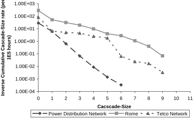
has a value of 105. Notice, from Fig. 1, that about 10 cascades of size greater than 4 occur in the combined Telco–Power system. However, the Power distribution net-work has about 8.87×10⁻³ of its cascades having a size greater than 4. So, the Power distribution network appears to contribute relatively little to the cascade size for the larger cascades. In contrast, there are about 2.53 cascades of size greater than 4 that occur in the Telco network; two orders of magnitude more than the related number for the Power distribution network. While this does not fully account for the number of cascades greater than 4 in the combined model it suggests that a significant number of relatively large cascades occur in other parts of the Rome model not depicted, i.e. the Power transmission network.
The “Strength of dependence” experiment explores the dependence of Power com-ponents on Telco comcom-ponents and vice–versa. The value for the Conditional
Power-substation Failure rate coefficient is set to 4800, which is higher than the correspond-ing value of 1000 in the base–level experiment. So, each power sub–station’s depend-ence on Telco–services in this experiment is almost 5 times stronger than in the base– level experiment. Contrastingly, the Conditional Telco-component failure rate
1.00E-04 1.00E-03 1.00E-02 1.00E-01 1.00E+00 1.00E+01 1.00E+02 1.00E+03
0 1 2 3 4 5 6 7 8 9 10 11
Cacscade-Size
In
v
e
rs
e
C
u
m
u
la
ti
v
e
C
a
s
c
a
d
e
-S
iz
e
ra
te
(
p
e
r
1
E
5
h
o
u
rs
)
[image:8.595.149.471.186.384.2]Power Distribution Network Rome Telco Network
Fig. 1. For the base–level experiment this graph depicts the sample–mean number of cascades
of size strictly greater than the indicated size (on the horizontal axis) that occur in each sub-network. For instance, the mean number of cascades that occurred in each of the sub–networks is given by the respective value of each graph corresponding to the cascade–size value of 0. So, the mean number of cascade events in the Power distribution network is 28.72, the mean num-ber of cascade events in the entire model is 285.12 and the mean numnum-ber of cascade events in the Telco network is 83.18.
The Power distribution network still contributes relatively little to the large cas-cades. There is no noticeable change, even though a change exists, in the contribution of Power distribution cascades to the total number of cascades in the model. The Telco network appears to exhibit a rapid drop from a frequency of 75.1 for single
graphs are arguably similar there is, nevertheless, a strict ordering between the graphs for “large” cascades (cascades with sizes greater than 6). “Large” cascades are strictly less likely to occur in the base–level experiment. Similar orderings are visible and more pronounced for the cascade–size distributions in both the Telco network and the Power distribution network. In particular, consider the Power distribution network (see Fig. 4), where the ordering is maintained and, additionally, the distributions ap-pear to diverge. One of the distributions is fairly linear on a log-linear plot and the other has approximately 2 linear regimes (one between cascade sizes 1 and 3 and the other between 4 and 6). This suggests 3 exponential laws governing the cascade-size distributions, with one of the distributions having 2 distinct laws characterizing it. Statistical tests of significance and estimating the parameters for these laws is of im-mediate interest. In summary, globally there appears to be little effect on cascade – size distributions from a weaker dependence of Telco components on Power services and stronger dependence of Power nodes on Telco services. Locally, however, there are differences between the distributions.
1.00E-03 1.00E-02 1.00E-01 1.00E+00 1.00E+01 1.00E+02 1.00E+03
1 3 5 7 9 11
Cascade-Size
C
a
s
c
a
d
e
-S
iz
e
R
a
te
(
p
e
r
1
E
5
h
o
u
rs
)
Power Distribution Network Rome Telco Network
Fig. 2. Cascade–size distribution for each sub–network in the “Strength of dependence”
ex-periment
In the “levels of abstraction” experiment we use a relatively naïve algorithm for power–line overloading on the cascade–size distributions, replacing the Linearized
DC approximation to AC power flow. A Binomial probability distribution randomly trips power–lines, given the failure of a power component. For the occurrence of cas-cades in each network will it matter that we are using an extremely simplistic algo-rithm to model power–line trips? If it does, how significant is the change in model behaviour? The value of the parameter Conditional probability of power-line
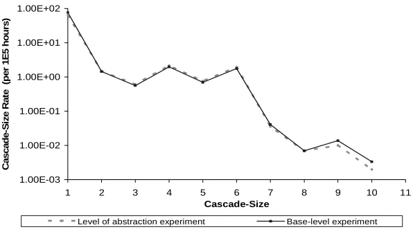
[image:9.595.167.452.328.523.2]comparable with 28⋅72 for the base–level experiment. The distributions for the Telco network are visibly almost identical (see Fig. 5). On the other hand, the power distribution network exhibits significant differences. A clear ordering exists, with the base–level experiment having an order of magnitude more occurrences of “large” cas-cades. The shape of the distributions both appear to be approximately linear and par-allel on a log-linear plot. Thus, again the data suggests an exponential relationship characterising the cascade size-distributions.
In conclusion, we note that while a significant change in strength of dependence noticeably affected the Cascade-size distributions for the sub-networks, the impact on the whole model was pronounced only for very large cascades. Also, the use of an ex-tremely simplistic algorithm for power line trips had a significant impact in the power distribution network but was negligible in the Telco network.
1.00E-02 1.00E-01 1.00E+00 1.00E+01 1.00E+02 1.00E+03
0 1 2 3 4 5 6 7 8 9 10 11
Cascade-Size
In
v
e
rs
e
C
u
m
u
la
ti
v
e
C
a
c
s
c
a
d
e
-S
iz
e
r
a
te
(
p
e
r
1
E
5
h
o
u
rs
)
[image:10.595.136.459.317.509.2]Strength of dependence experiment Base - level experiment
Fig. 3. Comparison of the Inverse, Cumulative Cascade–size rates for the Rome model.
5
Conclusion and future work
This paper presents a quantitative approach to modelling interdependencies in CIs and results from applying the approach to a non-trivial case-study, the Rome Power-Telco system developed within the EU IP IRRIIS.
dependence between various adverse events (e.g. failures of the modelled component) and risks of environmental disruptions (e.g. natural disasters, extreme weather condi-tions, etc.) but also to study the impact and challenge various assumptions about these. 1.00E-04 1.00E-03 1.00E-02 1.00E-01 1.00E+00 1.00E+01 1.00E+02
0 1 2 3 4 5 6 7 8
Cascade-Size In v e rs e C u m u la ti v e C a s c a d e -S iz e r a te (p e r 1 E 5 h o u rs )
Strength of dependence experiment Base-level experiment
Fig. 4. Comparison of the Inverse, Cumulative, Cascade–size rates for the Power distribution
network. 1.00E-03 1.00E-02 1.00E-01 1.00E+00 1.00E+01 1.00E+02
1 2 3 4 5 6 7 8 9 10 11
Cascade-Size C a s c a d e -S iz e R a te (p e r 1 E 5 h o u rs )
[image:11.595.160.448.213.379.2]Level of abstraction experiment Base-level experiment
Fig. 5. Comparison of Cascade – size distributions for the Telecommunications network.
[image:11.595.142.440.452.621.2]in some cases the behaviour of ‘low fidelity’ models is close to the behaviour of more sophisticated models (i.e. low fidelity models can offer an acceptable accuracy). This result seems important, because it opens up a practical way of modelling very large CIs with a reasonable accuracy.
In the light of these results we propose a future modelling approach in which a network of CIs is decomposed into manageable parts. Comparative studies (between high and low fidelity models, as described above) of these parts may then be applied so that the low-fidelity models can be tuned to model accurately the behaviour of the modelled sub-systems. Then, from the perspective of each CI, the network of CI may be modelled by combining acceptable low-fidelity models of some parts with high fi-delity models of other parts. Although such an approach seems plausible further work is needed to validate that the thus composed model will still be accurate. We intend to attack this issue in our future work.
In addition, the work demonstrates that a range of parameter values can give simi-lar model behaviour, depending on what aspects of the model are of interest. Very dif-ferent parameter values gave the same total number of cascades in the model. How-ever, the tails of the cascade-size distributions for the whole model and the power distribution network exhibited divergence. This suggests that in parameterizing such models for use in practice care must be taken since the effect of different parameter values is to produce “regimes of agreement” between the models. In the case we ob-served the models may diverge for large cascades but agree reasonably well for small cascades. The magnitude of this effect differed between networks.
In the current work, as a first approximation, static load profiles were used in the study. Dynamic load profiles that capture daily, or seasonal, variations in load may have the effect of significantly changing the probability of large-scale cascades. We will experiment with, and study the effects of, dynamic load profiles as an extension of the current work.
A related problem is addressing aspects of ‘observability’ of the state of the entire CI. The Rome system consists of networks, operated by organisations which may have detailed knowledge of their own network but very limited knowledge of the state of the networks operated by other operators. Approaches for dealing with such limited observability are of practical interest. We have scoped in [12] an approach to on-line risk estimation (RE) based on the probabilistic models described in this paper. Vali-dating RE in terms of achievable accuracy of risk predictions (i.e. whether the periods with predicted high risk of disruption will indeed tend to be highly positively corre-lated with actual disruptions) is a problem, which we are currently working on.
In addition to the relative confidence intervals used for determining acceptable convergence of the estimated distribution data points further statistical tests of signifi-cance will be carried out on the data to increase confidence in the results. Also, the data suggests a number of exponential relationships governing some of the cascade-size distributions. The parameters for these laws will be estimated as part of future work.
Acknowledgements
6
References
1. Bloomfield, R., et al., Report on Service Oriented Interdependency Analysis
(IRRIIS Project Deliverable D2.2.4). 2007, City University London: London. 2. Bloomfield, R., et al., Infrastructure interdependency analysis: an
introduc-tory research review. 2009, Adelard: London.
3. Boccaletti, S., et al., Complex networks: Structure and dynamics. Physics Reports, 2006. 424: p. 175-308.
4. Reka., A. and A.L. Barabasi, Statistical mechanics of complex networks. Re-views of Modern Physics, 2002. 74.
5. Pederson, P., et al. Critical Infrastructure Interdependency Modeling: A
Sur-vey of U.S. and International Research. 2006 [cited INL/EXT-06-11464]. 6. Schläpfer, M., T. Kessler, and W. Kröger. Reliability Analysis of Electric
Power Systems Using an Object-oriented Hybrid Modeling Approach. in
Proceedings of the 16th Power Systems Computation Conference. 2008. Glasgow.
7. U.S.-Canada Power System Outage Task Force. Final Report on the August
14, 2003 Blackout in the United States and Canada: Causes and Recommen-dations. 2004 [cited; Available from: https://reports.energy.gov/.
8. Board, B.M.I.I. The Buncefield Incident, 11 December 2005: The final
re-port of the Major Incident Investigation Board. 2004 December 2008 [cited; Available from: http://www.buncefieldinvestigation.gov.uk/index.htm. 9. IRRIIS. Integrated Risk Reduction of Information-based Infrastructure
Sys-tems. 2006-2009 [cited.
10. IRRIIS deliverable D2.2.4.,``Report On Service Oriented Interdependency Analysis''. 2007 [cited; Available from: http://www.irriis.org.
11. IRRIIS deliverable D2.2.2., ``Tools and techniques for interdependency
analysis''. 2007 [cited; Available from:
http://www.irriis.org/File.aspx?lang=2&oiid=9138&pid=572.
12. IRRIIS deliverable D2.2.6, "Preliminary Interdependency Analysis (PIA) as a service-oriented approach towards LCCI Interdependency Analysis (report and prototype)". 2009.
13. Rinaldi, S.M., J.P. Peerenboom, and T.K. Kelly, Identifying, Understanding,
and Analyzing Critical Infrastructure Interdependencies. IEEE Control Sys-tems Magazine, 2001. 21(6): p. 11-25.
14. Pearl, J., Probabilistic Reasoning in Intelligent Systems. 1988: Morgan Kaufmann, Palo Alto, CA.
15. Sanders, W.H., et. al., The Mobius Manual. 2008.
16. Sanders, W.H. and J.F. Meyer. Stochastic Activity Networks: Formal
Defini-tions and Concepts. in Lectures on Formal Methods and Performance
Analysis, First EEF/Euro Summer School on Trends in Computer Science. 2000. Berg en Dal, The Netherlands: Springer, Berlin, 2001.