DEVELOPMENT AND APPLICATION OF TEST CASES FOR COMPARING
VERTICAL GROUND HEAT EXCHANGER MODELS
Michel Bernier
1, Michaël Kummert
2,
Stéphane Bertagnolio
31
École Polytechnique de Montréal, Département de Génie Mécanique, Montréal, Canada
2
ESRU, Department of Mechanical Engineering, University of Strathclyde. United Kingdom
3
Laboratoire de Thermodynamique, Université de Liège, Belgique.
ABSTRACT
The main objective of this paper is to establish a set of test cases for analytical verifications and inter-model comparisons of ground heat exchanger (GHX) models used in building simulation programs. Several test cases are suggested. They range from steady-state heat rejection in a single borehole to varying hourly loads with large yearly thermal imbalance in multiple borehole configurations. The usefulness of the proposed test cases is illustrated by running them with different GHX models.
This comparison exercise has shown that 1-D models compare favourably well with the more elaborate 3-D models for relatively small simulation periods. The cyclic heat rejection/collection test has revealed some small deficiency in the load aggregation scheme of a particular model. Finally, the use of the asymmetric (cooling-dominated) load profile test case for a bore field composed of 100 boreholes revealed that the borehole wall temperature predicted by two GHX models can differ by as much as 10oC after a 30 year simulation.
KEYWORDS
Modeling, ground heat exchanger, simulations, test cases, heat pumps.
INTRODUCTION
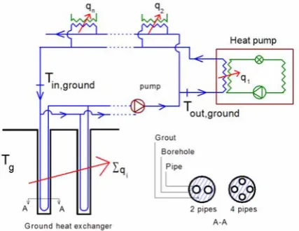
Ground-coupled heat pump (GCHP) systems are now routinely installed to provide space conditioning in a wide range of applications from small residences to large commercial buildings. A schematic representation of such a system is shown in Figure 1. The operation of the system is relatively simple: a pump circulates a heat transfer fluid in a closed circuit from the ground heat exchanger (GHX) to a heat pump (or a series of heat pumps).
Typically, GHX consists of boreholes that are approximately 100 m deep and have a diameter of 10-15 cm. The number of boreholes in the bore field can range from one for a residence to several dozens in commercial applications. As shown in Figure 1, two or four tubes are inserted in boreholes,
with fluid going down in one tube (or two in the case of a four tube configuration) and up the other(s). The volume between these pipes and the borehole wall is usually filled with grout to enhance heat transfer from the fluid to the ground.
In heating mode, heat pumps transfer heat from the fluid loop to the building and the GHX acts as a heat source. The total energy transferred from the fluid loop to the heat pumps (Σqi) represents the
amount of heat extracted from the ground. In cooling mode, heat pumps transfer heat from the building to the fluid loop and the GHX acts as a heat sink.
The temperature level in the fluid loop depends on three main factors: the amount of heat collected (rejected) into the ground; the far field ground temperature, Tg, and the effective thermal
[image:1.595.318.532.431.596.2]resistance between the fluid temperature in the borehole and Tg.
Figure 1 Typical closed-loop ground-coupled heat pump system.
LITERATURE REVIEW
Several models are available to simulate the behaviour of GHX in bore field sizing programs or in building simulation programs.
Tout,ground is the required output (usually at one hour
time intervals). Despite these different objectives, both approaches use similar techniques to model ground heat transfer.
Sizing software packages for GHX have been compared for residential and commercial applications. In the case of residential applications, Shonder et al. (1999) examined two cases; one where the GHX length was determined by the heating load and the other by the cooling load. The authors show that the GHX length predicted by six different sizing programs are within ±7% and ±16% of each other for these two cases. Comparison was also made with the DST model (Hellström, 1996) which was referenced by the authors as being the “benchmark”. Shonder et al. (2000) also used the DST benchmark in their comparison for larger commercial applications. They compared four sizing programs. Three of these programs agree with the benchmark lengths to within ± 12%.
Validation or comparison of GHX models used in hourly simulation programs have been performed on a limited basis. In his pioneering work, Eskilson (1987) showed that his g-functions were in good agreement with the well-known line-source analytical solution (Carslaw and Jaeger 1947, Ingersol et al. 1954). Yavuzturk and Spitler (1999) extended the work of Eskilson to short-time steps. They validated their approach with an experimental data set. Unfortunately, the data acquisition started three months after the start of the operation of the system. Furthermore, the data set contained gaps. Despite these deficiencies their model agrees reasonably well with experimental data. Fisher et al. (2006) compared the short-time step model with Hellström’s (1991) line source model for a composite heat extraction function. The maximum difference (1.7°C) between the two approaches occurred when a pulse load was periodically applied. They also compared their results with experimental data from Hern (2002). This comparison included the GHX model as well as the heat pump model. The resulting system model predicted ground heat transfer rate to within 6% of the experimental results.
Huber and Pahud (1999) ran a series of 20 test cases to compare two models. Their tests covered several operating conditions and bore field geometries. Their inter-model comparison proved to be helpful in revealing differences in the models. Bernier et al. (2004) have compared their GHX model with the DST model. They note that both models are in good agreement. However, extensive testing was not performed. Finally, to the knowledge of these authors, there are no carefully
monitored and publicly available GHX data that could be used for model validation.
OBJECTIVE
The objective of this paper is to present a series of test cases that could be used to validate GHX models.
Several test cases are suggested. They range from steady-state heat rejection in a single borehole to varying hourly loads with large yearly thermal imbalance in multiple borehole configurations. The usefulness of the proposed test cases is illustrated by running them with different GHX models. Based on the established BESTEST (Judkoff and Neymark, 1995) terminology, test presented here fall into the categories of “analytical verification” and “comparative testing”.
IMPACT OF INACCURATE
PREDICTIONS ON ANNUAL HEAT
PUMP ENERGY CONSUMPTION
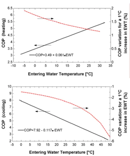
GHX models used in building simulation programs predict the hourly (or even sub-hourly) fluid return temperature from the ground. Given that precise evaluation of the annual heat pump energy consumption is intimately linked to the fluid temperature prediction, it is worthwhile to examine the impact of inaccuracies on the heat pump COP and annual energy consumption. Figure 2 shows average coefficients of performance (COP) as a function of heat pump entering water temperature (EWT). These curves were obtained by curve fitting COP data from ten commercially available 3-ton (10.5 kW) heat pumps units (Bernier, 2006). As indicated in the graph, the slope of the COP curve is +0.061 and -0.117 for heating and cooling, respectively. Thus, for each 1°C variation in EWT, the COP will increase by 0.061 and decrease by 0.117 in heating and cooling, respectively. Also shown on Figure 2 are curves representing the relative COP variation for an increase of 1°C of the EWT. For example, for EWT=10°C, a 1°C increase in EWT leads to a COP increase of 1.49% in heating mode.
concept of Equivalent Full Load Hours (EFLH) in cooling and heating is used (Carlson et al. 2002).
Figure 2 Average COP values as a function of the heat pump entering water temperature.
Table 1 Effect of an over prediction of 2°C in EWT1
EFLH cooling/heating
Error in yearly heat pump energy consumption
Cooling only 6.5%
2500/500 4.6% 1000/1000 1.7% Heating only -3.1%
1 Based on EWT of 5°C and 35°C in heating and cooling, respectively.
It is reasonable to expect that energy consumption results obtained from energy simulation programs should have an accuracy of the order of ± 5%. If this value is used then, according to data presented in Figure 2 and Table 1, GHX models should predict the EWT (Tout,ground in Figure 1) to within
approximately 2°C.
TYPICAL BOREHOLE GEOMETRY
Figure 3 shows a typical 4×4 bore field and the nomenclature that will be used in this paper. B is the centre-to-centre borehole spacing. The depth is H and the active heat exchange area starts at a distance D from the ground surface. The ground is caracterised by its thermal conductivity, kg, and
thermal diffusivity, αg, and by the undisturbed
ground temperature, Tg . As shown in Figure 3, the
fluid circuitry is usually arranged so as to form a reverse-return circuit ensuring that each borehole
receives an equal share of the total flow rate,
m
&
total. The inlet temperature to each borehole is equal to the return temperature from the heat pumps, Tin,ground. The outlet tempertaure from the borefield,Tout,ground, represents the average borehole outlet
temperature. Thus, the total amount of heat rejected/collected in the ground, Σqi ,is simply
given by:
, ,
( )
i total p out ground in ground
q m C T T
[image:3.595.317.514.177.454.2]∑ = & − (1)
Figure 3 Typical bore field geometry
In the sections that follow the variable q (without indexes) is used. It represents the amount of heat rejected/collected per unit length. It should not be confused with the total heat rejected/collected (Σqi
in Figure 1).
GHX MODELS
readily available to the authors. Second, these models are significantly different in their treatment of ground heat transfer, thermal interaction among boreholes, and load aggregation. Therefore, they offer a wide range of possibilities to evaluate the relevancy of test cases.
g-function of Eskilson
Eskilson (1987) has shown that, for a fixed value of D ( = 5m in his studies ) and for a fixed number of boreholes and bore field aspect ratio (B/H), the bore hole wall temperature (Tb in Figure 3) is given by:
( / , / ) 2
b g s b
g
q
T T g t t r H
k
π
= − × (2)
where ts is a characteristic time = (H2/9αg) and “g”
represents Eskilson’s g-function. These g-functions have been generated for a number of geometrical configurations and are available in the literature (Eskilson, 1987). The “g-functions” are usually presented graphically as a function of ln(t/ts) for a
particular bore field geometry and aspect ratio and for a given value of rb/H. Given the thermal
response for a single value of q, the response to any heat rejection/extraction value of q can be determined by dividing the heat rejection/extraction into a series of step functions, and superimposing the response to each step function. Finally, the g-functions of Eskilson account for the three-dimensional nature of heat transfer in the bore field.
DST model
Hellstrom (1991) developed a 3-D simulation model for seasonal thermal energy storage with vertical ground heat exchangers. The model incorporates the spatial superposition of three parts: a so-called ‘‘global’’ temperature difference between the heat store volume and the undisturbed ground temperature, a temperature difference from the ‘‘local’’ solution around the heat store volume, and a temperature difference from the ‘‘local’’ steady-flux part. The model was implemented in TRNSYS (Hellström el al. , 1996). The DST model implemented in TRNSYS assumes that the boreholes are placed uniformly within a cylindrical storage volume of ground. The user specifies the desired spacing between boreholes and the program calculates the corresponding storage volume. Thus, the user cannot specify a rectangular geometry such as the one presented in Figure 3.
Cylindrical Heat Source
The cylinder heat source (CHS) method was developed by Carslaw and Jaeger (1947). This method uses an analytical solution for one-dimensional radial heat conduction from a cylinder subjected to a constant heat flux at its radius. The CHS method can be used with varying heat rejection by using the principle of temporal superposition (Bernier, 2001).
MLAA model
Bernier et al. (2004) have developed a GHX model which superimposes the local solution to a global solution to account for thermal interaction among boreholes. The 1-D solution of the cylindrical heat source is applied locally at each borehole. The thermal interaction is obtained by solving for the two-dimensional heat transfer in the bore field (heat transfer in the axial direction, i.e, along the borehole depth, is neglected). In order to reduce the computational effort associated with temporal superposition, the model incorporates a Multiple Load Aggregation Algorithm (MLAA). Furthermore, thermal interaction among boreholes is evaluated every two weeks to speed up calculations. The MLAA aggregates heating/cooling loads. It uses two major thermal history periods, referred to as “past” and “immediate.” The immediate thermal history (6 hours) is not aggregated, while the past thermal history is subdivided into four time intervals, with periods of the order of a day (24 hours), a week (168 hours), a month (360 hours), and years (remaining hours since the beginning of the simulation). For example, assume successive ground heat injection loads of 1000 Watts for 12 hours followed by 500 Watts for 18 hours. In its temporal superposition scheme, the MLAA will assume that the ground load is 500 Watts for the last six hours and that it has an average of 750 Watts for the 24 hour interval prior to the immediate 6-hour thermal history.
TEST CASES
GHX models differ in the way they calculate local (near the borehole) heat transfer, thermal interaction among boreholes, and load aggregation. Therefore, test cases need to evaluate models in at least these three areas.
As mentioned earlier, borehole sub-models are not considered in this paper. However, in the DST and MLAA models, it is difficult to bypass these sub-models without making significant code changes.
Therefore, for these two models the borehole thermal resistance was made artificially small by specifying a high thermal conductivity grout. Furthermore, a high fluid flow rate was specified. The combination of these two specifications made Tout,gorund and Tin,ground essentially equal to each other
and also equal to the borehole wall temperature, Tb.
SINGLE BOREHOLE
A) Constant heat rejection
[image:5.595.316.531.72.263.2]This test consists in injecting a constant amount of heat into the ground and calculating the resulting borehole wall temperature. This is the most basic test case. It can be considered to be an analytical verification of the g-function and DST models with the CHS analytical solution. Since the ground load is constant, temporal superposition and load aggregation are not tested. Furthermore, for a single borehole, thermal interaction is not an issue. The various parameters used for this test, which will be referred to the SB-A test, are given in Table 2.
Table 2
Parameters used for the single borehole constant heat rejection case (SB-A)
Parameter Value
H 110 m
rb 0.055 m
D 5 m
Tg 0°C
kg 1.3 W/m-K
q/2πkg -1 °C
Note that Tg and the ratio q/2πkg have been
conveniently set to 0°C and -1°C, respectively. Thus, according to equation 2, Tb corresponds
directly to the value of the g-function.
Figure 4 presents a comparison of the borehole wall temperature predicted by the four models for this test case. Since heat rejection is constant, it is convenient to present the results as a function of non-dimensional time, ln(t/ts). For reference,
assuming a typical ground thermal diffusivity of 0.0624 m2/day and the values listed in Table 2, values of ln(t/ts) of 0 and -2.3 correspond to periods
of 59 and 5.9 years after the start of the heat injection, respectively. As shown in this figure the MLAA and CHS models give identical results. Similarly, the g-function and DST models follow very similar trends. However, both group of models start to differ from each other when ln (t/ts) reaches
a value of approximately -4. The difference is around 0.1°C after 5.9 years and reaches 0.5°C after 59 years.
This difference stems from the fact that after a certain time, heat transfer in the ground is two-dimensional (radial and axial). Since the CHS and the MLAA are 1-D models (the MLAA reduces to a 1-D model for single borehole configurations) it is not suprising to see this discrepancy after a few years. It is also interesting to note that the g-function and the DST models tend to reach a steady-state as evidenced by the plateau in the
borehole wall temperature reached by both models for ln(t/ts) ~ 2.
Figure 4 Comparison of four models for the SB-A test case.
B) Symmetric cyclic heat rejection/collection
This test consists in imposing constant and symmetric cycles of heat rejection/collection. The values listed in Table 3 are used for this test. This leads to values of q/2πkg which alternate from +1°C
to -1°C each 24 hours. This test is used to compare the various models on their load aggregation capabilities.
Table 3
Parameters used for the cyclic heat rejection/collection case (SB-B)
Parameter Value
H 100 m
rb 0.05 m
D 5 m
Tg 0°C
kg 1.3 W/m-K
αg 0.0624 m2/day
q Cycle of +8.19 W/m for 24 hours then -8.19 W/m for 24 hours
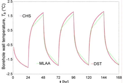
[image:5.595.315.528.593.736.2]Figure 5 Comparison of three models for the SB-B test case
As shown, the results of the CHS and DST models are almost indistinguishable. The MLAA follows the other two models except towards the changeover from heating to cooling and vice versa. The first occurrence of this discrepancy is apparent at hour 30. This is due to the load aggregation scheme of the MLAA which averages loads that are not part of the immediate (last 6 hours) thermal history.
C) Synthetic asymmetric load profile
This test, named SB-C, consists of calculating the resulting borehole wall temperature over long periods when the borehole is subjected to an asymmetric load profile. This load profile is generated using a mathematical function (Bernier et al. 2004) which is described in the appendix. The resulting load profile is shown in Figure 6 where negative values indicate heat rejection into the ground. This profile emulates a cooling-dominated load.
[image:6.595.315.525.310.710.2]Figure 6 Synthetic asymmetric load profile.
Figure 7 Comparison of the MLAA and DST models for the SB-C test case.
Simulations were performed with the MLAA and DST models using this load profile and the parameters listed in Table 3. Results are shown in Figure 7 for the last year of a 30 year simulation. As shown on the top portion of this figure, the DST and MLAA models agree with each other within approximately ± 1°C. Thus, both models seem to aggregate loads satisfactorily.
MULTIPLE BOREHOLES
Aside from testing the local (at the borehole) heat transfer and load aggregation over time, multiple borehole tests add one more difficulty, i.e. thermal interaction among boreholes. Bore field configurations of 2, 4 and 100 boreholes with B/H =0.05 will be compared for two different test cases.
A) Constant heat rejection
This test, named MB-A, uses the SB-A test parameters except that bore fields of 2 and 100 boreholes are considered. Results are shown on Figures 8 and 9. For the 2 boreholes configuration a difference of 0.7oC is observed for ln(t/ts) = 0. (i.e
[image:6.595.72.279.534.717.2]after a simulation time of 59 years). The jagged behavior of the MLAA method is explained by the fact that the thermal interaction is not calculated at every time step. Instead, it is calculated every 336 hours (2 weeks) and it remains constant over that period. Thus every two weeks, the borehole wall temperature experiences an abrupt increase associated with a recalculation of the thermal interaction among boreholes. As was noted in relation to Figure 4, the DST model and the g-function tend to reach a steady-state condition while the borehole wall temperature predicted by the MLAA model continues to rise. Clearly, the 2-D nature of the MLAA model limits its applicability to relatively small periods of simulations.
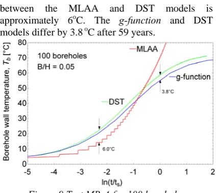
Figure 8 Test MB-A for 2 boreholes
between the MLAA and DST models is approximately 6oC. The g-function and DST models differ by 3.8 oC after 59 years.
Figure 9 Test MB-A for 100 boreholes
C) Synthetic asymmetric load profile
This test, named MB-C, uses the same load profile utilized for test SB-C, including the asymmetric load profile shown in Figure 6. Tests for 4 and 100 boreholes are presented in Figures 10 and 11 for the MLAA and DST models. The top portion of these figures indicates the difference between the DST and MLAA models.
Figures 10 shows that thermal interaction is not very strong in a 4 borehole configuration as the borehole wall temperature is marginally higher than for the single borehole configuration. The agreement between the MLAA and DST models is within approximately ± 1oC even after 30 years, a similar discrepancy to the one observed earlier in conjunction with Figure 7. Borehole thermal interaction is much more pronounced for 100 boreholes. With such a dense bore field, heat gets trapped in middle boreholes which tend to raise the overall borehole wall temperature.
Figure 10 Test MB-C for 4 boreholes
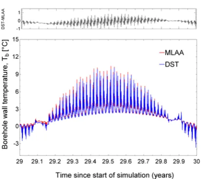
As shown on Figure 11, the MLAA overestimates the borehole wall temperature. This discrepancy is
[image:7.595.314.523.129.309.2]of the order of 10oC after 30 years. It is probably due to the fact that the MLAA does not account for heat exchange on the top and bottom of the storage volume.
Figure 11 Test MB-C for 100 boreholes
CONCLUSION
Several test cases for analytical verification and inter-model comparisons of GHX models are presented in this paper. They range from steady-state heat rejection in a single borehole to varying hourly loads with large yearly thermal imbalance in multiple borehole configurations.
The usefulness of the proposed test cases is illustrated by running them with different GHX models. This comparison exercise shows that 1-D models compare favourably well with the more elaborate 3-D models for relatively small simulation periods in the selected test cases. The cyclic heat rejection/collection test has revealed a small deficiency in the load aggregation scheme of a particular model. Finally, the use of the asymmetric (cooling-dominated) load profile test case for a bore field composed of 100 boreholes revealed that the borehole wall temperature predicted by two GHX models can differ by as much as 10°C after a 30 year simulation.
It is hoped that this work will help developing a much-needed test suite for GHX models. Finally, a good set of empirical values would certainly be an asset in the quest for improved validation tools for GHX models.
ACKNOWLEDGMENT
REFERENCES
Bernier, M. 2006. Closed-loop Ground-Coupled Heat Pumps Systems, ASHRAE Journal, Vol. 48, no.9, pp.12-19.
Bernier, M.A., Pinel, P., Labib, R., and R. Paillot. 2004. A multiple load aggregation algorithm for annual hourly simulations of GCHP systems, Int. J. of HVAC&R Research, 10 (4): 471-488.
Bernier M.A. 2001. Ground-Coupled Heat Pump System Simulation, ASHRAE Trans., vol. 106, pt. 1, pp. 605-616.
Carslaw, H.S., and J.C. Jaeger. 1947. Conduction of heat in solids, Oxford.
Carlson, S.W., Thornton, J.W. 2002. Development of Equivalent Full Load Heating and Cooling Hours for GCHPs, ASHRAE Trans. 107(2): 88-98.
Eskilson, P. 1987. Thermal analysis of heat extraction boreholes. Doctoral Thesis, Lund University, Sweden.
Fisher, D.E., Rees, S.J., Padmanabhan, S.K., Murugappan, A., 2006. Implementation and Validation of Ground-Source Heat Pump System Models in an Integrated Building System Simulation Environement, Int. J. of HVAC&R Research, 12 (3a): 693-710.
Hellström, G. 1991. Ground heat storage: Thermal analysis of duct storage systems. Lund, Sweden: University of Lund, Department of Mathematical Physics.
Hellström, G., Mazzarella, L., and D. Pahud. 1996. Duct ground storage model – TRNSYS version. Department of Mathematical Physics, University Of Lund, Sweden.
Hern, S.A. 2002. Design of an Experimental Facility for Hybrid Ground Source Heat Pump Systems, M.Ss. Oklahoma State University. Huber, A., Pahud, D. 1999. Erweiterung des
Programms EWS für Erdwärmesondenfelder, Bundesamt für Energie.
Ingersoll, L.R., O.J. Zobel, and A.C. Ingersoll. 1954. Heat conduction: With engineering and geological applications, 2d ed. McGraw-Hill. Judkoff, R., Neymark, J., 1995. IEA- BESTEST
and Diagnostic Method, NREL.
Piechowski, M. 1998. Heat and Mass Transfer Model of a Ground Heat Exchanger: Validation and Sensitivity Analysis, Int. J. Energy Res., 22: 965-979.
Shonder, J.A., Baxter, V., Thornton, J.W. 1999. A New Comparison of Vertical Ground Heat Exchanger Design Methods for Residential Applications, ASHRAE Trans.105(2): 1179-1188.
Shonder, J.A., Baxter, V.D., Hughes, P.J., Thornton, J.W. 2000. A Comparison of Vertical Ground Heat Exchanger Design Software for Commercial Applications, ASHRAE Trans. 106 (1): 831-842.
Thornton, J.W., T.P. McDowell, J.A. Shonder, P.J. Hughes, D. Pahud, and G. Hellstrom. 1997. Residential Vertical Geothermal Heat Pump System Models: Calibration to Data. ASHRAE Trans. 103(2): 660-674.
Yavuzturk, C., and J.D. Spitler. 1999. A Short Time Step Response Factor Model for Vertical Ground Loop Heat Exchangers. ASHRAE Trans. 105(2): 475-485.
Yavuzturk, C., and J.D. Spitler. 2001. Field Validation of a Short Time-step Model for Vertical Ground-Loop Heat Exchangers. ASHRAE Trans. 107(1): 617-625.
APPENDIX
The synthetic profiles shown on Figure 6 are obtained using the following mathematical function:
(
)
(
)
{
}
(
)
( ) 8760 ( ) 8760; , , ( 1) ; , ,
( 1)
cos 4380
D floor x C
D floor x C
y f x A B C
abs f x A B C
E
D
signum π x F G
⎛ − ⎞ ⎜ ⎟ ⎝ ⎠ ⎛ − ⎞ ⎜ ⎟ ⎝ ⎠ = + − × + × − × ⎛ ⎛ ⎛ − ⎞+ ⎞⎞ ⎜ ⎜ ⎜⎝ ⎟⎠ ⎟⎟ ⎝ ⎠ ⎝ ⎠ where
(
)
3 1; , , sin ( ) sin ( )
12 4380
168 1
cos 1 sin ( )
168 i 84 84
f x A B C A x B x B
C C i i
x B i π π π π π = = − − − + − × − ⎛ ⎞ ⎛ ⎞× ⎜ ⎟ ⎜ ⎟ ⎝ ⎠ ⎝ ⎠ ⎡⎛ ⎞ ⎛ ⎛ ⎞ ⎞ ⎛ ⎛ ⎞⎞⎤ ⎜ ⎟ ⎜ ⎟ ⎜ ⎟ ⎢⎝ ⎠ ⎜⎝ ⎝ ⎠ ⎟ ⎜⎠ ⎝ ⎝ ⎠⎟⎠⎥ ⎣