Predicting Category Intuitiveness With the Rational Model, the Simplicity Model, and the Generalized Context Model

City, University of London Institutional Repository

Citation

:

This is the unspecified version of the paper.

This version of the publication may differ from the final published

version.

Permanent repository link:

Link to published version

:

Copyright and reuse:

City Research Online aims to make research

outputs of City, University of London available to a wider audience.

Copyright and Moral Rights remain with the author(s) and/or copyright

holders. URLs from City Research Online may be freely distributed and

linked to.

Predicting category intuitiveness with

the rational model, the simplicity

model, and the Generalized Context

Model

Emmanuel M. Pothos

Department of Psychology

Swansea University

Todd M. Bailey

School of Psychology

Cardiff University

in press: JEP: LMC

Please address correspondence to Emmanuel Pothos, Department of Psychology,

Swansea University, Swansea SA2 8PP, UK, or to Todd Bailey, School of

Psychology, Cardiff University, Cardiff CF10 3AT, UK. Electronic mail may be sent

at [email protected] or [email protected]

Running head: GCM category intuitiveness; Word count (running text, excluding

Abstract

Naïve observers typically perceive some groupings for a set of stimuli as more

intuitive than others. The problem of predicting category intuitiveness has been

historically considered the remit of models of unsupervised categorization. In

contrast, this paper develops a measure of category intuitiveness from one of the most

widely supported models of supervised categorization, the Generalized Context

Model (GCM). Considering different category assignments for a set of instances, we

ask how well the GCM can predict the classification of each instance on the basis of

all the other instances. The category assignment that results in the smallest prediction

error is interpreted as the most intuitive for the GCM—we call this way of applying

the GCM unsupervised GCM. The paper then systematically compares predictions of

category intuitiveness from the unsupervised GCM and two models of unsupervised

categorization, the simplicity model and the rational model. We found that the

unsupervised GCM compares favorably to the simplicity model and rational model.

This success of the unsupervised GCM illustrates that the distinction between

supervised and unsupervised categorization may have to be reconsidered. However,

no model emerges as clearly superior, indicating that there is more work to be done in

understanding and modeling category intuitiveness.

Keywords: supervised categorization, unsupervised categorization, exemplar theory,

Introduction

The distinction between supervised and unsupervised categorization has been central

to the development of categorization theory in cognitive science. Supervised

categorization concerns predicting how novel instances will be classified, with respect

to a set of existing categories; such predictions can be typically carried out with

impressive accuracy. Prominent classes of supervised categorization models include

the exemplar theory (Medin & Schaffer, 1978; Nosofsky, 1988; Van Vanpaemel &

Storms, 2008), prototype theory (Hampton, 2000; Minda & Smith, 2000; Posner &

Keele, 1968), and the general recognition theory (Ashby & Perrin, 1988). Supervised

categorization typically involves training procedures with corrective feedback. By

contrast, in a typical unsupervised categorization experiment participants are asked to

divide some stimuli into categories which are intuitive, without any corrective

feedback.

Interest in unsupervised categorization largely originates from the notion of

category coherence (Murphy & Medin, 1985). Why do certain groupings of objects

form psychologically intuitive categories, but other groupings are nonsensical? For

example, most cultures have concepts such as happiness or animal. By contrast, a

grouping which includes the Eiffel Tower, children under five, and apples would be

considered entirely nonsensical. Murphy and Medin (1985) suggested that a category

is coherent if it fits well with our overall understanding of the world; they argued that

explanations based on similarity are inadequate (cf. Heit, 1997; Lewandowsky,

Roberts, & Yang, 2006; Wisniewski, 1995). Unfortunately, creating categorization

models on the basis of general knowledge is extremely difficult (e.g., Fodor, 1983;

Pickering & Chater, 1995; but see Griffiths, Steyvers, & Tenenbaum, 2007 or

people do use similarity in unsupervised categorization, at least in some cases.

Accordingly, some researchers have developed unsupervised categorization models

which are based on similarity (e.g., Compton & Logan, 1993; Love, Medin, &

Gureckis, 2004; Milton & Wills, 2004; Pothos & Chater, 2002).

Unsupervised categorization involves two slightly separate problems: first,

identifying the classification for a set of stimuli, which would be preferred by naïve

observers. For example, in Figure 1, the preferred classifications for the dots are the

ones indicated by the continuous curves (here and elsewhere, points represent objects

and the axes are assumed to correspond to dimensions of some putative internal

mental space; similarities are inversely related to distances). A second problem in

unsupervised categorization is, given a classification for a stimulus set and another for

a different stimulus set, deciding which one is more intuitive. In Figure 1, the

classification on top should be perceived as more intuitive compared to the

classification in the bottom panel (this is because the difference of within- versus

between-category similarity in the top panel is higher than in the bottom; Pothos &

Chater, 2002). In other words, if real stimuli are created after the Figure 1 points,

participants are likely to identify the top classification as preferred more frequently

and with more confidence, compared to the bottom classification. In principle, a

model of category intuitiveness provides the basis for a model of unsupervised

categorization, under the assumption that the most intuitive categorization will also be

the preferred one.

---FIGURE 1---

A main objective of this work is to examine predictions of category

intuitiveness from computational models of unsupervised categorization, for a range

this kind. This is an important shortcoming, given the strong intuitions we can have

about which categorizations are more intuitive than others. We consider category

intuitiveness predictions from the rational model (Anderson, 1991; Sanborn, Griffiths,

& Navarro, 2006) and the simplicity model (Pothos & Chater, 2002). The inclusion of

these two models has been partly motivated by the fact that they can readily produce a

measure of category intuitiveness (this is not always the case with models of

unsupervised categorization; e.g., see Compton & Logan, 1993).

Unsupervised and supervised categorization have typically been assumed to

correspond to different psychological processes and the related research traditions

have been mostly separate. A model is typically proposed as either a model of

supervised categorization or a model of unsupervised categorization. However, this is

an assumption which may be inappropriate. The other main objective of this paper is

to show that a measure of category intuitiveness can be derived from one of the best

known models of supervised categorization, Nosofsky’s Generalized Context Model

(GCM; Nosofsky, 1988, 1989, 1991, 1992). The version of the GCM which can

produce predictions of category intuitiveness will be referred to as unsupervised

GCM, to reflect the fact that, in this mode of application, the GCM assesses the

intuitiveness of a particular classification instead of classifying new instances with

respect to existing categories. Predictions of category intuitiveness from the GCM

will be compared to those from the rational model and the simplicity model.

Unsupervised GCM

The GCM predicts classification probabilities for a set of test stimuli based on their

similarity to a set of previously seen training stimuli. The GCM is described by two

XB B XA A XA A X A P         ) |

( ………(1a)





XA c w y y

/ 1 1 | | exp  ……….(1b)

P(A|X) is the probability of making a category A response, given instance X (the 

terms are category biases and XA is the sum of the similarities between X and all the

A exemplars). This is Luce’s (1963) choice rule; it sometimes involves an exponent to

the similarities. In equation (1b), c is a sensitivity parameter, r is a Minkowski

distance metric parameter, q determines the shape of the similarity function, wk are

dimensional attention weights, and y’s are item coordinates. The input to the GCM

consists of the coordinates of a set of training stimuli, information about the

assignment of the stimuli to categories, and the coordinates of a set of test stimuli. On

the basis of this information, the parameters of the GCM are adjusted so as to predict

as closely as possible empirically determined probabilities of how the test items are

classified. An error term can be computed as 



i i i P O O ln

2 , where Oi are the target

probabilities and Pi the predicted probabilities from the model; the summation ranges

over all the test items. Target probabilities typically correspond to how participants

classify test items into training categories. This equation computes a likelihood ratio

chi-square statistic (e.g., see Hahn, Bailey, & Elvin, 2005). We refer to this error term

as a log likelihood error term.

How could the GCM compute (relative) category intuitiveness? Suppose that

in the top panel of Figure 1 we want to evaluate the intuitiveness of classification {1,

2, 3,4, 5, 6}{7, 8, 9} versus {1, 2, 3}{4, 5, 6, 7, 8, 9}. In evaluating classification {1,

4, 5, 6, are in category {1, 2, 3,4, 5, 6} with 100% probability and likewise for items

7, 8, 9 and category {7, 8, 9}. In other words, exemplars are assigned to categories in

accordance with the category structure being evaluated and GCM fits are computed

on this basis. A main insight in this paper is that when the GCM self-classifies a set of

stimuli in this way, the corresponding error term can be interpreted as a measure of

category intuitiveness. We postulate that where the error term is lower, then the

corresponding classification is more consistent with the assumptions about

categorization ingrained in the GCM and that, therefore, such classifications are

considered more psychologically intuitive by the GCM. For example, self-classifying

the Figure 1 items relative to the classification {1, 2, 3,4, 5, 6}{7, 8, 9} should be

associated with a very small error term, as the two categories are well separated. By

contrast, self-classification relative to {1, 2, 3}{4, 5, 6, 7, 8, 9} should lead to a high

error term. These results correspond to the obvious impression that, for the stimuli in

Figure 1, classification {1, 2, 3,4, 5, 6}{7, 8, 9} is psychologically more intuitive than

{1, 2, 3}{4, 5, 6, 7, 8, 9}.

This scheme constitutes a proposal for using the GCM to produce a measure

of category intuitiveness (cf. Feldman, 2004; Pothos & Chater, 2002). We believe that

given a measure of category intuitiveness one can create a full model of unsupervised

categorization, but this is an objective for future work. One can ask what kind of

category structures will be predicted as more intuitive by the GCM. For example,

Feldman (2004) suggested that the Boolean complexity of concepts defined through

logical expressions determines their psychological intuitiveness. Work on basic level

categorization has assumed that category structure can be understood in terms of the

ratio of within category similarity to between category similarity (Murphy, 1991;

1992), or a tradeoff between cue and category validities (Jones, 1983). The

corresponding claim for the unsupervised GCM is that an intuitive classification will

be possible for a set of stimuli if there are groupings which maximize within category

similarity, both with respect to the original representation of the stimuli, and the

various transformations for this representation allowed by the GCM parameters

(suppression of dimensions and stretching/ compression of psychological space). This

latter characteristic particularly distinguishes the GCM from other unsupervised

categorization models based on similarity. The unsupervised and supervised versions

of the GCM are based on the same equations, but applied to answer different

questions. In the former case, the computed error term is interpreted as category

intuitiveness, in the latter case classification probabilities of novel instances are

predicted. Crucially, in the unsupervised GCM parameters are not adjusted to match a

particular pattern of empirical results (parameters are determined by item coordinates,

so that parameter search is guided by a prerogative to achieve an intuitive

classification), while in the supervised GCM parameters are specified so as to achieve

particular probabilities for the classification of new instances.

So, our measure of category intuitiveness from the GCM is based on the same

equations as the standard GCM (cf. Love, 2002). This is an important point, since it

shows how a model which has been considered the hallmark of supervised

categorization can be directly applied to unsupervised categorization. The specific

details of how we applied the GCM are standard. The city block (r=1) and the

Euclidean (r=2) metrics are the only metrics that have received psychological

motivation, and likewise for the exponential (q=1) and Gaussian (q=2) forms of the

similarity function. It has not been possible to motivate more specific values of r and

Category biases were allowed to vary freely between zero and one, subject to the

constraint that they summed to one, and likewise for the attentional weights. The

sensitivity parameter, c, determines the extent to which the classification of an

instance is influenced by remote exemplars or not. When c is very small, all

exemplars will have an effect on how a test item is classified. As c increases in size,

classification of a test item will be influenced primarily by its nearest neighbor

amongst the training items, or, in a situation where the training items are the same as

the test items, just by itself. This latter situation is pathological, so we required the

unsupervised GCM to classify each stimulus on the basis of all the other stimuli in a

stimulus set only. Given this requirement, in all our simulations the default approach

was to allow c to vary freely between zero and infinity. We will later examine directly

whether the unsupervised GCM can function adequately with an unrestricted c.

It is by no means obvious at the outset that our proposal will necessarily

succeed. A common criticism for the GCM (and similar models) is that its parameters

allow it too much flexibility in fitting empirical data (Olsson, Wennerholm, &

Lyxzen, 2004; Myung, Pitt, Navarro, 2007; Navarro, 2007; Nosofsky, 2000; Nosofsky

& Zaki, 2002; Smith, 2007; Smith & Minda, 1998, 2000; 2002; Yang &

Lewandowsky, 2004). Accordingly, one can wonder whether our suggestion for the

unsupervised GCM might fail because the GCM can perfectly describe any

assignment of stimuli into categories (regardless of whether the corresponding

classifications are more or less intuitive). The burden is on us to demonstrate that not

only is this not the case, but that the unsupervised GCM can perform comparably with

established models of unsupervised categorization.

Many models of unsupervised categorization (including the unsupervised GCM and

the simplicity model) rely on similarity. It is interesting to include in the comparisons

a model that makes no explicit reference to similarity. Anderson’s (1991) rational

model adopts a category utility approach. In other words, it assumes that categories

are formed because they are useful to us, specifically because they allow us to infer

unknown information about novel instances (cf. Corter & Gluck, 1992; Gosselin &

Schyns, 2001; Jones, 1983; Medin, 1983; Murphy, 1982).

The rational model is an incremental, Bayesian (cf. Tenenbaum & Griffiths,

2001; Tenenbaum, Griffiths, & Kemp, 2006) model of unsupervised categorization. It

assigns a new stimulus with feature structure F to whichever category k makes F most

probable. For example, a new object with many features of a ‘cat’, would be assigned

to the category of cats, since the feature structure of the object is most probable given

this category membership.

We implemented the continuous version of the rational model, which assumes

that stimuli are represented in terms of continuous dimensions (for more details see

Anderson, 1991; Anderson & Matessa, 1992). The continuous version allows the most

direct comparison with the unsupervised GCM, since the latter also assumes

continuous dimensions. In the rational model, the probability of classification of a

novel instance into category k depends on the product P(k)P(F|k). P(k) is given by

equation (3a):

cn c cn k

P k

  

) 1 ( ) (

………(3a)

In equation (3a), nk is the number of stimuli assigned to category k so far, n is the total

number of classified stimuli, and c is a coupling parameter. The coupling parameter

Thus, c indirectly determines the number of categories that the rational model will

produce for a stimulus set. The probability that the new object comes from a new

category is given by

cn c c P     ) 1 ( 1 ) 0

( . P(F |k)is computed as in equation (3b):





i

i x k

f k

F

P( | ) ( | )

………..……….(3b)

where i indexes the different dimensions of variation of the stimuli and x indicates

the different values dimension i can take. That is, f_i(x|k) is the probability of

displaying value x on dimension i in category k, and is approximated by

)

/

1

1

,

(

ai

t









2

i

 are given by equations (3c) and (3d).

n y n i _   0 0 0     ………(3c) n y n n s n i        0 2 0 0 0 2 2 0 0 2 ) ( ) 1 (        ………..………....(3d)

-3d- is the variance for classifying into the i dimension. This tells us how much it

‘matters’ whether a stimulus has a particular value on dimension i or not, for

classification into a particular category.

In these equations, _i ₀ n, _i ₀ n, n is the number of observations in

category k, y is their mean along dimension i, and s2 is their variance. Finally,

0

0 1 

   , ₀ is the halfway point of the range of all instances and ₀ is the square

of a quarter of the range (Anderson, personal communication).

It is possible to introduce a dimensional weighting mechanism in the rational

each dimension is weighted by w1, w2 etc., to indicate the relative importance of the

dimensions in classifying a new item. In other words,

_{The question is what kind of weighting scheme is going to be optimal for}

the rational model. Taking logs in the above equation, we have:

Suppose that . Then,

clearly, the weight combination which maximizes is w1=0, w2=1. In other

words, in the rational model, optimal dimensional weighting corresponds to assigning

a weight of 1 to the most useful dimension and a weight of 0 to all the other

dimensions (so that, in contrast to the GCM, graded weighting is never optimal for the

rational model). Therefore, in the simulations below, where we refer to the ‘rational

model with dimensional selection’, we assess the probabilities for the predicted

classifications along all one-dimensional projections.

Note that the standard rational model can compute the probability for a

classification, given a particular order of the items. However, all the empirical

examples below assume concurrent presentation of the stimuli. Sanborn, Griffiths,

and Navarro (2006) provided algorithms for the rational model, which approximate

classification probabilities from the rational model, as if all items had been presented

concurrently. Sanborn et al.’s examination of their algorithms was shown to both have

desirable normative properties and outperform the standard rational model in specific

empirical cases. Specifically, we used the Gibbs sampler algorithm to compute the

probability for the most probable classification for a stimulus set. Moreover, we

adapted the algorithm to compute the probability of any particular classification (not

necessarily the most probable one) for a stimulus set. In either case, higher

Simplicity model

The simplicity model of unsupervised categorization (Pothos & Chater, 2002, 2005;

Pothos & Close, 2008) differs from the rational model and the unsupervised GCM in

a number of interesting ways. First, the simplicity model is non-metric (a metric space

is not assumed), while this is not the case for the other two models. Second, the

simplicity model has no free parameters, a characteristic which contrasts most sharply

with the unsupervised GCM. Third, the simplicity model aims to maximize within

category similarity and minimize between category similarity, but only the former

constraint is relevant to the unsupervised GCM. Finally, the simplicity model is

currently the only model which has been applied to data from entirely unconstrained

categorization procedures; it is therefore interesting to compare it with the rational

model and the unsupervised GCM against such data.

According to the simplicity model, more intuitive categories are ones that

maximize within category similarity and minimize between category similarity (cf.

Rosch and Mervis, 1975). The model is specified within a computational framework

based on the simplicity principle (Chater, 1996, 1999). The first step is to compute the

information content of the similarity structure of a set of items without categories.

This is done by assuming that every pair of stimuli is compared with every other pair.

For example, suppose that we have four stimuli, labeled by 1,2,3,4. Then, similarity

information would be encoded as similarity(1,2)>similarity(1,3),

similarity(1,2)<similarity(1,4), etc., with each comparison requiring one bit of

information to specify whether the first pair is more similar or less similar than the

second (assuming no exact equalities).

Categories are defined as imposing constraints on the similarity relations

all similarities between categories. For example, suppose that we decide to place

stimuli 1,2 in one category and stimuli 3,4 in a different category. Then, our definition

of categories implies that similarity(1,2)>{similarity(1,3), similarity(1,4)} and that

similarity(3,4)>{similarity(1,3), similarity(1,4)}. Thus, the codelength for the

similarity structure for a set of stimuli can be reduced by using categories, if the

constraints specified by the categories are numerous and, generally, correct (note that

equalities in similarity relations do not falsify the constraints; Hines, Pothos, &

Chater, 2007). If in u constraints there are e incorrect ones, the number of bits of

information required to correct the errors is given by equation (2a).

_         )! ( ! ! log ) 1 (

log2 2

e u e

u

u ………..…(2a)

Moreover, we have to take into account the information-theoretic cost of specifying a

particular category structure of n categories for r objects, which is given by

)) , ( (

log₂ Part r n , where Part(r,n) is given by equation (2b).

! )! ( ) ( ) 1 ( ) , ( 1

0 n v v

v n n r Part r n v v    



Overall, there is a codelength without categories and a codelength with categories.

The ratio of the latter to the former indicates how much codelength reduction is

afforded by the use of categories; it is typically reported as a percentage and referred

to as just ‘codelength’. The lower its value, the more intuitive a particular category

structure is predicted to be. The lowest possible value of codelength is about 50%.

When trying to identify the most intuitive classification from scratch, the simplicity

model employs a search algorithm akin to those in agglomerative clustering

Analyses

Our analyses are divided in three parts. First, all three models are examined with a

simple toy stimulus set. For the rational model and the simplicity model, this exercise

illustrates the way they are applied and some basic implementational assumptions.

Regarding the unsupervised GCM, this exercise is more important, since it

corresponds to a preliminary test of whether the model can capture some obvious

intuitions about category intuitiveness. Second, we examined a range of classic

stimulus sets from the supervised categorization literature, on the assumption that

category learnability is related to intuitiveness. Third, we considered data from studies

which employed an entirely unsupervised categorization procedure.

Toy stimulus set/ illustration of the models’ operation

Four stimulus sets were created to assess the three models with respect to the

straightforward intuition that well-separated, coherent categories should be more

intuitive than less-separated ones. Each stimulus set was intended to correspond to a

category structure composed of two clusters. The stimulus sets differed on how close

the two clusters were to each other, with category prototypes being 2, 3, 4, or 5 units

apart. The two most extreme stimulus sets are shown in Figure 2; the other stimulus

sets were in between these extremes.

Unsupervised GCM intuitiveness values were obtained as log likelihood error

terms, which reflect the deviance between the intended assignment of stimuli into

categories and the predicted assignment by the GCM. A lower error term implies that

the corresponding classification is considered more intuitive. Constrained

optimization of the GCM parameters was done with the fmincon Matlab function

(version R2007b). We examined the log likelihood error term for a particular

lowest error term was taken to be the intuitiveness value from the unsupervised

GCM). To facilitate comparisons with other models, we normalized the log likelihood

values for all category structures onto a 0-1 scale (with 0 corresponding to least

predicted intuitiveness and 1 corresponding to the greatest intuitiveness), through the

transformation

min max

min 1

 

 X , where X is the log likelihood error for any of the four

category structures, min is the least log likelihood error (of these four values), and

max is the greatest error. By carrying out this (or analogous) transformation for the

predictions from all models, we can derive an impression of how the models compare

with each other. The normalized scores have been used in all figures, raw model

predictions in the tables.

Simplicity model predictions were given as codelength values, so that a lower

codelength indicates a more intuitive classification. Codelength values typically range

between 50% and 100%. Recall that the input to the simplicity model is not item

coordinates, but rather information of which pairs of similarities are greater or smaller

than others. In order to derive such information from item coordinates, a distance

metric has to be assumed. Consistently with previous examinations of the simplicity

model (e.g., Pothos & Chater, 2002, 2005), we opted for the Euclidean metric. The

Euclidean metric is an appropriate default choice, since it corresponds better to the

way physical distances are perceived psychologically. Of the models considered, the

simplicity model was the most straightforward to run, requiring less than a minute per

stimulus set. Simplicity values were transformed onto a 0-1 scale as above.

Using Sanborn et al.’s (2006) adaptation of the rational model, it is possible to

identify the best classification for a set of items and compute the probability for any

particular classification—as noted, these probabilities can be interpreted as

of iterations for different stimulus sets (at least 10,000), with a view to ensure that not

more than 10 hours were required per stimulus set. Sample spacing was set to 20. For

the coupling parameter we employed the commonly used value of 0.5. Finally, for the

rational model with dimensional selection, intuitiveness values corresponded to the

most probable classification regardless of whether all dimensions or a particular

dimension were employed.

All models correctly predicted that category structures for which the two

categories are closer together should be less intuitive, compared to category structures

for which the categories are further apart (Table 1). This is hardly an exciting

prediction, but nonetheless an important basic test that the models are consistent with

expectations in such an intuitive case. Note that the rational model with dimensional

selection correctly predicts that the optimal dimension in all cases is dimension 1 (in

other words, the probability of the best possible classification along dimension 1 is

greater than the corresponding probability along either dimension 2 or both

dimensions). In this straightforward case, there is agreement between the rational

model and the rational model with dimensional selection. Regarding the simplicity

model, the lowest possible codelength in this case is 51.6; as noted, the exact value

will somewhat depend on the particular classification. Also, the worst possible

codelength is 117.9, well over 100. This reflects the fact that when the prototypes are

only two units apart, the costs associated with correcting errors in the constraints

specified by the classification are so high, that we are actually better off describing

the similarity information without categories.

The behavior of the models can be seen in Figure 3, where each of the model

measures has been transformed on a 0 to 1 scale. While such a transformation

appreciating model similarities and differences (in this case, for example, the fact that

the unsupervised GCM and the simplicity model rise quickly to their highest value,

while the rational model’s rise is more gradual).

---FIGURES 2,3, TABLE 1---

Supervised categorization data

Supervised categorization data can be used to derive estimates of category

intuitiveness in two ways. First, we assume that if classification A is more difficult to

learn than classification B, then, in an unsupervised context, classification A will be

considered more intuitive compared to B. The empirical evidence supports this

assumption. Colreavy and Lewandowsky (in press) found no difference between a

supervised categorization condition and a matched unsupervised one, in terms of

strategy development and rate of learning (see also Griffiths, Christian, & Kalish,

2008). Love (2002) reached the opposite conclusion, but his supervised and

unsupervised stimulus sets were not directly comparable, and the learning task was

not entirely equivalent to an unsupervised categorization one.

Second, consider categories A and B and a new instance X. Suppose that

participants are more likely to classify X into category A than B. Since participants

classified X with category {A} rather than {B}, they must think that the overall

grouping {A,X}{B} must be more intuitive than the alternative grouping {A}{B,X}.

Therefore, we can assume that classification {A,X}{B} is more intuitive than

{A}{B,X}. We can then examine whether the unsupervised categorization models

consider{A,X}{B} as more intuitive compared to {A}{B,X}. Note that the

application of the unsupervised GCM to such data is very different from the standard

application of the GCM, where the objective is to predict classification probabilities

Finally, methodologically, one can ask whether the categories employed in

supervised categorization research may be so unstructured that they would never be

created in a spontaneous fashion. But, this is not a problem since the difference in

relative intuitiveness between two classifications, however unstructured, can always

be empirically examined: participants’ spontaneous classifications should be more

similar to the one which is predicted to be more intuitive.

Shepard, Hovland, and Jenkins (1961). Shepard et al. (1961) considered the

difficulty of learning six binary classifications with stimuli made of three binary

dimensions (Table 2). Classification 1 is simple to learn because it covaries perfectly

with the first dimension of the stimuli. Classification 2 reflects an ‘exclusive OR’

(non linear) category structure in its first two dimensions, while the third dimension

constitutes random noise. Classifications 3, 4, and 5 can be described by

one-dimensional rules with exceptions and require attention to all three dimensions.

Classification 6 also requires attention to all three dimensions, but in this case there

are no obvious regularities. Shepard et al. reported that the cumulative error rate

conforms to the following ordering: Classification 1 (easiest) < Classification 2 <

{Classifications 3, 4, 5} < Classification 6 (most difficult). This result has become a

benchmark for assessing models of supervised categorization (e.g., Love et al., 2004;

Kurtz, 2007; Nosofsky & Palmeri, 1996).

---TABLES 2, 3, FIGURE 4---

As discussed, we assumed that more intuitive classifications should be easier

to learn (the results of Griffiths et al., 2008, support this assumption in the case of the

Shepard et al. data, with a kind of unsupervised induction task). The unsupervised

GCM, the simplicity model, and the rational model were applied by computing the

raw results are shown in Table 3 and normalized predicted intuitiveness scores are

shown in Figure 4. The unsupervised GCM performed better than both the simplicity

model and the rational model. The unsupervised GCM correctly predicted that

Classifications 1, 2 should be the most intuitive, 3,4,5 of intermediate intuitiveness,

and, finally, that Classification 6 should be the least intuitive. Note that

Classifications 1 and 2 are not distinguished (the former should be more intuitive than

the latter). The simplicity model considered all classifications highly unintuitive; the

codelength values produced were very close to 100, predicting that participants

receiving these stimulus sets would be unlikely to spontaneously produce the Shepard

et al. classifications. The model does predict that Classification 1 should be the most

intuitive and Classification 6 the least intuitive one. However, the simplicity model

was confused by Classification 2, which was predicted to be less intuitive than 3,4,5.

The rational model had a similar problem: as with the simplicity model, the rational

model correctly predicted Classifications 1 and 6 to be the most and least intuitive,

respectively; however, it incorrectly predicted Classification 2 to be less intuitive than

Classifications 3,4,5. The same pattern of results was predicted by the rational model

with dimensional selection, even though the optimal dimension varied in different

cases. To sum up, with the Shepard et al. data, the unsupervised GCM outperformed

the models of unsupervised categorization.

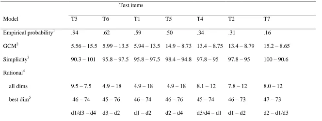
5-4 category structure. The 5-4 category structure (Medin & Schaffer, 1978) has been

extensively explored in the context of the debate between prototype and exemplar

theory (e.g., Johansen & Kruschke, 2005; Nosofsky, 2000; Smith & Minda, 2000; but

see Homa, Proulx, & Blair, 2008). Medin and Schaffer (1978) reported classification

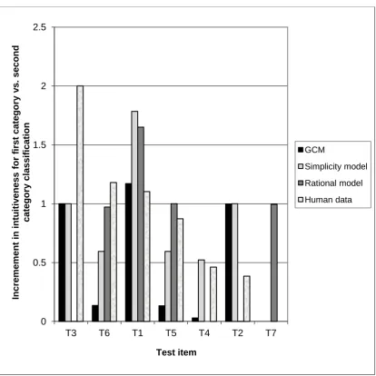
probabilities for seven test items (Table 4) and, as discussed, we can use these

categorization model, two computations were made for each test item: One with the

test item assigned to the first category and another with the test item assigned to the

second category. These two computations corresponded to two intuitiveness values

for each item. The difference between these two values should correspond to the

classification probabilities reported by Medin and Schaffer (1978).

---TABLES 4, 5, FIGURE 5---

The results are shown in Table 5 and Figure 5. To create Figure 5, for the

unsupervised GCM we computed the difference in log likelihood error for the

classification when the first test item was assigned to the first category minus the log

likelihood error for the classification when the first test item was assigned to the

second category; and likewise for the other test items. (In other words, we subtracted

the values in each of the cells in Table 5.) Subsequently, these differences were

converted onto a uniform scale, as in the other examples (in this case, the scale was

0—2; model predictions corresponded to differences between two intuitiveness

values, and such differences could be negative). An analogous procedure was adopted

for the other models. Correlating classification probabilities and the differences in

predicted intuitiveness values, for the unsupervised GCM, the simplicity model, the

rational model, and the rational model with dimensional selection respectively, we

obtained: -.857, -.960, .068, -.412. Note that a negative correlation is in the predicted

direction for the unsupervised GCM and the simplicity model, since for these models

lower values (lower error or lower codelength) correspond to more intuitive

classifications and, hence, should be associated with higher classification probabilities

in Medin and Schaffer’s data. The GCM and the simplicity model competently

describe the Medin and Schaffer (1978) data; however, the rational model had

Linear separability. A classification is linearly separable if a straight line (or the

equivalent in more than two dimensions), can divide all the items which belong to one

category from all items which belong to another. Linear separability is an important

consideration in categorization, since exemplar theory is consistent with non-linearly

separable categories, but this is not the case for prototype theory. The empirical

results have been somewhat ambiguous (Ashby & Maddox, 1992; Kalish,

Lewandowsky, & Kruschke, 2004; Kemler Nelson, 1984; Kemler Nelson, 1984;

Olsson, Enkvist, & Juslin, 2006; Medin & Schwanenflugel, 1981; Ruts, Storms, &

Hampton, 2004; Shepard et al., 1961; Smith, Murray, & Minda, 1997; Wattenmaker,

1995). The latest research with schematic stimuli indicates that linearly separable

categories are more intuitive (Blair & Homa, 2001). Of the category structures Blair

and Homa used, most relevant are the ones with four categories each, in which each

category had nine points (these were the largest stimulus sets). The linearly separable

category structure was referred to by Blair and Homa as LS9 and the non-linearly

separable one as NLS9. Blair and Homa reported an advantage of the LS9

classification relative to the NLS9 one, in terms of ease of learning.

We modeled the LS9 vs. NLS9 contrast reported by Blair and Homa (2001).

Each LS9 category was based around a prototype and nine ‘high distortion’ items

from the prototype. Each NLS9 category was based around the same prototypes, six

‘low distortion’ items from the prototype, and one low distortion item from each of

the other three prototypes (the items from the other prototypes result in non-linearity).

Blair and Homa reported the coordinates of six items from each prototype in three

dimensions, which were derived from similarity ratings (Blair, personal

communication). To approximate the Blair and Homa stimulus sets, the coordinates of

prototype. Then, we computed the average distance between the prototypes and

low/high distortion items, and so created enough low/high distortion items to

approximate the LS9 and NLS9 category structures (Appendix). We created two more

extreme stimulus sets, referred to as LS9X and NLS9X, in which the prototype

coordinates were changed so that the least distance between any two prototypes would

be at least 1.5 times the distance between a prototype and a high distortion item. The

LS9, NLS9 stimulus sets can only be said to approximate the actual Blair and Homa

stimulus sets. Therefore, we examined linear separability of each stimulus set with a

series of logistic regressions attempting to predict category membership (Ruts et al.,

2004). Our re-creation of LS9 is not linearly separable (probably because categories

are too close to each other), but it is a lot more so compared to NLS9. Moreover, the

new stimulus set LS9X is linearly separable.

---TABLE 6, FIGURE 6---

The empirical finding we aimed to model was that LS9 was easier to learn

compared to NLS9. Although there are no relevant empirical results for LS9X and

NLS9X, we tentatively assume that for LS9X increasing the distance between

category prototypes would make a category structure more salient (a straightforward

assumption), but this would not be the case for NLS9X (a more controversial

assumption). The results are shown in Table 6 and Figure 6. The unsupervised GCM

and the simplicity model successfully predicted a difference between LS9 and NLS9

and a more pronounced difference between LS9X and NLS9X. Note that using the

unsupervised GCM to predict category intuitiveness is a different computation from

that corresponding to the standard GCM and, so, our results do not bear on the fact

that Blair and Homa (2001) could not identify satisfactory (standard) GCM fits for the

classifications were extremely unlikely, and maybe this obscured any finer differences

due to linear separability.

Unsupervised categorization data

Compton & Logan (1999). Compton and Logan (1999) reported extensive data on

judgments of category intuitiveness, in an entirely unsupervised categorization task.

They presented participants with diagrams of dots, as in Figure 1 (but without any

curves), and asked participants to classify the dots in a way that seemed immediately

natural and intuitive, by drawing curves to indicate their groupings. There were no

constraints at all as to how the items should be classified (including no constraints on

the number of groups; cf. Murphy, 2004). Compton and Logan measured category

intuitiveness in terms of classification variability, that is, the number of unique

classifications for each diagram shown to participants, so as to examine whether

classification variability changed when the arrangement of dots in a diagram was

transformed (e.g., reflected or rotated). Compton and Logan employed 48 unique

diagrams, which consisted of 12 examples for each numerosity of dots from 7 to 10,

inclusive (each participant classified 144 diagrams, the 48 original ones and various

transformations of them). Each unique diagram was created by randomly arranging

the appropriate number of dots in a 40x40 grid.

The categorization procedure of Compton and Logan somewhat deviates from

the standard procedure in unsupervised categorization experiments: participants drew

lines around points, instead of classifying stimuli as separate entities. For example,

the classification of dots in a diagram will be affected by the nearest neighbor

structure in the diagram; participants would rarely classify in the same cluster dots

which are far away from each other. By contrast, in standard unsupervised

classification of highly dissimilar items into the same group is sometimes observed.

However, Compton and Logan (1999) is currently the most extensive report of

unsupervised categorization results. Moreover, perceptual grouping processes in

Compton and Logan’s experiment is arguably very similar to the grouping by

similarity, postulated by models such as simplicity and the GCM: in both cases, the

assumption is that participants will prefer groupings which enhance within category

similarity. Finally, some researchers have argued that such dot diagrams is a valid

way to study unsupervised categorization (Pothos & Chater, 2002).

Compton and Logan only reported the diagrams for which they observed the

two highest and two lowest classification variability values in each of their two

experiments; we read off the item coordinates from the diagrams (Appendix), so as to

examine whether the predictions of the unsupervised categorization models are

consistent with the highest/ lowest classification variability results reported by

Compton and Logan: there should be less classification variability for stimulus sets

for which the models can identify more intuitive classifications.

---TABLE 7, FIGURE 7---

The simplicity model and the rational model can identify the best possible

classification for a set of items. In the case of the simplicity model, we employed the

agglomerative search algorithm described in Pothos and Chater (2002) and for the

rational model the Gibbs sampler algorithm in Sanborn et al. (2006), which computes

the most probable classification for a set of items, in a way that approximates

concurrent presentation of the items.

Regarding the unsupervised GCM, we have no algorithm to identify the

preferred classification from scratch. Therefore, we examined the log likelihood error

model with dimensional selection, and K-means two- and three-cluster algorithms

(excluding some all-inclusive categories identified by the rational model, since such

categories are pathological for the unsupervised GCM); the intuitiveness prediction

from the GCM for a stimulus set corresponded to the lowest identified log likelihood

error term overall. In this case, we also examined a modification for the unsupervised

GCM, for which the sensitivity parameter was fixed to a constant value (we chose

c=0.5, noting that which value of c is suitable will depend on the coordinate units).

Why is this consideration relevant in this case, but not in the case of the stimulus sets

from supervised categorization studies? In unsupervised research, the classifications

considered are typically chosen to be intuitive to naïve observers. Accordingly,

without a restriction on c, the GCM can always stretch the representational space in

such a way that the corresponding classification is maximally intuitive.

Psychologically, by restricting the sensitivity parameter, we suggest that participants

spontaneously classify an item not just by considering its single nearest neighbor, but

in relation to many of the other items as well (this seems highly plausible in the case

of the Compton & Logan results, and also the Pothos & Chater results, considered

next).

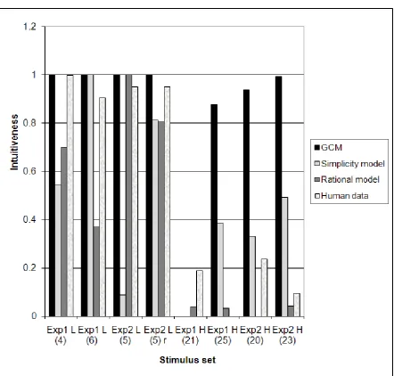
The results are shown in Table 7 and Figure 7. Note first that the standard

unsupervised GCM is unable to discriminate between the intuitive and unintuitive

stimulus set, but this is not so when a restriction in the sensitivity parameter is

introduced. We next correlated the classification variability results reported by

Compton and Logan with the intuitiveness values generated from each model. These

(Pearson) correlations were for the unsupervised GCM, .319, the unsupervised GCM

with a c restriction, .407, the simplicity model, .430, the rational model, -.032, and the

higher values from the unsupervised GCM and the simplicity model correspond to

less intuitive categories, but higher values from the rational model to more intuitive

categories). Of these correlations, the one involving the rational model with

dimensional selection probabilities was the highest, showing that allowing

dimensional selection in the rational model is a key modification regarding the

model’s explanatory power. Moreover, the unsupervised GCM with c restricted

performs better than the unrestricted GCM. Specifically, it correctly identifies the four

low variability stimulus sets as more intuitive than all the four high variability ones.

Pothos and Chater (2002). Pothos and Chater examined four 10-item stimulus sets

for which there were differing intuitions about the most intuitive classification

(Appendix). In the first one, there were two well-separated clusters of equal size

(referred to as ‘two clusters’). In the second one, there were also two well-separated

clusters, but one was larger than the other (referred to as ‘big small’). In the third

stimulus set there were three well-separated clusters (‘three clusters’). Finally, there

was little classification structure in the last stimulus set (referred to as ‘little’).

We consider Experiment 2 of Pothos and Chater, whereby item coordinates

were mapped onto (separable) dimensions of physical variations, to create stimulus

pictures that were printed on separate sheets of paper and given to participants to be

sorted into groups that were “intuitive and natural”. No constraints were imposed on

participants’ classifications (e.g., participants could use as many clusters as they liked,

they could see the stimuli in any order or way they liked, and they could make

changes in their classifications). This represents the most naturalistic unsupervised

categorization study we found in the published literature. Pothos and Chater employed

28 participants and measured classification performance in terms of three indices, the

the number of robust distinct classifications (these are the distinct classifications with

a frequency greater than one), and the frequency with which the best possible

classification was produced. Because of the small sample, these three measures did

not correlate very well with each other; Pothos and Chater considered the last two as

the most valid. We derived two separate rank orderings for the four stimulus sets from

these two measures, which we subsequently added together to obtain an overall rank

ordering for the observed intuitiveness of different stimulus sets. For the ‘two

clusters’, ‘big, small’, ‘three clusters’, and ‘little’ stimulus sets, the summation of the

ranks for these two measures produced 3, 2, 5, and 7 respectively, whereby a lower

number indicates higher category intuitiveness.

---TABLE 8, FIGURE 8---

Unsupervised GCM category intuitiveness predictions were computed for the

classifications predicted by the simplicity model, the rational model with dimensional

selection, and K-means two-cluster and three-cluster algorithms. As before, we

explored the version of the unsupervised GCM with and without restricting the

sensitivity parameter; for the rational model we employed the Sanborn et al. (2006)

algorithms. The simplicity model was applied to the stimulus sets by searching for the

best possible classification on the basis of item coordinates. The results are shown in

Table 8 and Figure 8. The simplicity model and the restricted unsupervised GCM

accurately predicted the ordinal ordering of empirical classification intuitiveness in

Table 8, but this was not the case for the unrestricted unsupervised GCM (which

failed to discriminate between any of the stimulus sets). Finally, the rational model

with dimensional selection was in much closer correspondence to the empirical results

Conclusions

Naïve observers can often have very compelling intuitions that a particular grouping

for a set of stimuli may be more appropriate than another. Therefore, understanding

the computational basis for such intuitions appears an important objective for models

of unsupervised categorization. One aim of this paper was to examine predictions

about category intuitiveness, from computational models of categorization, against a

series of studies from the categorization literature.

Models of unsupervised categorization which can readily produce a measure

of category intuitiveness are the rational model and the simplicity model and so these

two models were tested in our analyses. Future work could fruitfully include

additional models, such as Schyns’ (1991) self-organizing neural network, which was

used to model category emergence, Compton and Logan’s (1993, 1999) perceptual

grouping approach to unsupervised categorization, or Love et al.’s (2004; Gureckis &

Love, 2002) SUSTAIN model, which assumes two slightly separate mechanisms for

supervised and unsupervised categorization (respectively, an explicit error term and

surprisingness with a principle of similarity). Finally, there has been an extensive

literature on statistical clustering (e.g., Fisher and Langley, 1990; Krzanowski &

Marriott, 1995), which looks relevant to studies of unsupervised categorization. Such

models could serve as psychological models of categorization, after some additional

theoretical elaboration.

Another aim of this paper was to explore the possibility that a measure of

category intuitiveness could be derived from a supervised model of categorization, the

GCM. In our adaptation of the GCM, a candidate classification for a set of items is

examined by considering how well the intended classification of each item can be

computed, which indicates the ability of the GCM to describe the candidate

assignment of items to categories. We postulated that when this error term is lower,

then the corresponding classification is more consistent with the assumptions of the

GCM about categorization, so that such a classification would be predicted (by the

GCM) to be more psychologically intuitive. Both the supervised and unsupervised

GCM are based on exactly the same equations, but are applied differently. The

unsupervised GCM computes a number which can be interpreted as category

intuitiveness, while the supervised GCM predicts classification probabilities for novel

instances. Crucially, in the unsupervised GCM no parameter fitting is taking place

relative to empirical data (parameters are searched so as to identify the best possible

classification for a set of stimuli), while in the supervised GCM parameters are

specified so as to achieve particular probabilities for the classification of new

instances.

The unsupervised GCM favors groupings of items that maximize within

category similarity. The crucial difference between the unsupervised GCM and

models such as the simplicity one is that similarity groupings are assessed not just

against the initial/ unprocessed dimensional representation of the items, but against all

possible derivative representations, which would be forthcoming from dimensional

weighting, stretching/ compression of psychological space etc. This representational

flexibility is, of course, the hallmark of GCM predictions and its characteristic which

has allowed it to provide impressive fits to empirical data. It is also a characteristic

that has provoked some criticism since, if the GCM is proved to be too flexible, then

its explanatory power would be limited. Accordingly, a possible way in which our

demonstration could have failed would be if the unsupervised GCM could predict

this was not the case, and the accuracy of the predictions from the unsupervised GCM

compared favorably from those of the rational model and the simplicity model.

One can ask whether the unsupervised GCM is meant to be understood as a

full model of unsupervised categorization. For a full model of unsupervised

categorization what is needed is a criterion of category intuitiveness and a search

algorithm which can use this criterion to identify the optimal classification for a set of

stimuli from scratch. The unsupervised GCM fulfills only the first requirement. It can

be used to compute the predicted category intuitiveness for a stimulus set, a prediction

which can be compared with the ones from the rational model and the simplicity

model. However, the current formulation of the unsupervised GCM fails the second

requirement. To appreciate why this is the case, consider first how the simplicity

model (equally for the rational model) works. The simplicity model can easily

identify the predicted most intuitive classification for a set of stimuli from scratch,

with simple search algorithms which take the stimulus configuration and identify the

classification which best optimizes the model’s criterion for category intuitiveness.

For the unsupervised GCM, the problem is that there is no single stimulus

configuration, but rather an infinite number of possible ones, defined by stretching/

compressing psychological space or different relative attentional weighting of the

item dimensions (in other words, the situation is like having different stimulus sets,

the original one and all possible transformations of the original one, as allowed by the

GCM parameters). Thus, in the case of the unsupervised GCM the search space is

much more extensive, making optimization of its criterion for category intuitiveness

intensive and difficult (so that, for example, the straightforward agglomerative

algorithm which works for the simplicity model will not work for the unsupervised

Regarding the results of our simulations, all models performed reasonably

well, but no model could be identified as clearly superior when compared to the

others. More work needs to be done in order to model category intuitiveness in a

satisfactory way. For example, with the Shepard, Hovland, Jenkins (1961) data, the

unsupervised GCM performed better than both the simplicity model and the rational

model. In the case of the 5-4 category structure (Medin & Schaffer, 1978), the

simplicity model came out ahead, with the unsupervised GCM providing the second

best fit. In the case of comparing Blair and Homa’s (2001) LS/ NLS category

structures, the simplicity model and the unsupervised GCM could both provide a

perfect account of the empirical findings. Compton and Logan (1999) provided one of

the early studies with an entirely unsupervised categorization procedure. The best

description for their results was from the rational model with dimensional selection.

The unrestricted unsupervised GCM was too powerful for this data. It was necessary

to constrain the sensitivity parameter before the unsupervised GCM could accurately

predict an intuitiveness difference between the low and high variability stimulus sets

(cf. Stewart & Brown, 2005; Olsson et al., 2004). Finally, the restricted unsupervised

GCM and the simplicity model could account for Pothos and Chater’s (2002) data,

and the results from the rational model with dimensional selection were in close

correspondence too.

The relative success of the unsupervised GCM calls into question the

distinction between supervised and unsupervised categorization which has dominated

the literature. We showed that a model of supervised categorization could be

straightforwardly adapted to make predictions about category intuitiveness. Also, the

converse situation is implied in our demonstration: models of unsupervised

studies, by assuming that when a classification is more difficult to learn then it should

be less intuitive (cf. Colreavy and Lewandowsky, in press). It is therefore possible

that both supervised and unsupervised categorization could be described within the

same mathematical framework (e.g., the GCM), noting, however, that behavioral or

neuroscience data may show these to correspond to distinct psychological processes

(e.g., cf. Ashby & Ell, 2002; Ashby & Perrin, 1988; Nomura et al., 2007; Zeithamova

& Maddox, 2006; see also Love et al., 2004). Future work will hopefully address

these exciting issues, as well as extend formalisms like the rational model and the

Acknowledgments

This research was partly supported by ESRC grant R000222655 to EMP. We would

like to thank Peter Hines, Mark Johansen, Matt Jones, Rob Nosofsky, Amotz

Perlman, David Smith, and Safa Zaki. We are grateful to John Anderson for his help

with the implementation of the continuous version of the rational model, to Adam

Sanborn for helping with the Gibbs sampler, and to Mark Blair for his suggestions for

specifying the LS/ NLS stimulus sets, from the Blair & Homa study.

References

Anderson, J. R. (1991). The Adaptive Nature of Human Categorization. Psychological

Review, 98, 409-429.

Anderson, J. R. & Matessa, M. (1992). Explorations of an incremental, Bayesian

algorithm for categorization. Machine Learning, 9, 275-308.

Ashby, G. F. & Perrin, N. A. (1988). Towards a unified theory of similarity and

recognition. Psychological Review, 95, 124-150.

Ashby, G. F. & Maddox, W. T. (1992). Complex decision rules in categorization:

contrasting novice and experienced performance. Journal of Experimental

Psychology: Human Perception and Performance, 18, 50-71.

Ashby, G. F. & Ell, S. W. (2002). Single versus multiple systems of category

learning: Reply to Nosofsky and Kruschke (2002). Psychonomic Bulletin &

Review, 9, 175-180.

Blair, M. & Homa, D. (2001). Expanding the search for a linear separability constraint

on category learning. Memory & Cognition, 29, 1153-1164.

Chater, N. (1996). Reconciling Simplicity and Likelihood Principles in Perceptual

Chater, N. (1999). The Search for Simplicity: A Fundamental Cognitive Principle?

Quarterly Journal of Experimental Psychology, 52A, 273-302.

Colreavy, E. & Lewandowsky, S. (in press). Strategy development and learning

differences in supervised and unsupervised categorization. Memory & Cognition.

Compton, B. J. & Logan, G. D. (1993). Evaluating a computational model of

perceptual grouping. Perception & Psychophysics, 53, 403-421.

Compton, B. J. & Logan, G. D. (1999). Judgments of perceptual groups: Reliability

and sensitivity to stimulus transformation. Perception Psychophysics, 61,

1320-1335.

Corter, J. E. & Gluck, M. A. (1992). Explaining Basic Categories: Feature

Predictability and Information. Psychological Bulletin, 2, 291-303.

Feldman, J. (2000). Minimization of Boolean complexity in human concept learning.

Nature, 407, 630-633.

Fisher, D., & Langley, P. (1990). The structure and formation of natural categories. In

Gordon Bower (Ed.), The Psychology of Learning and Motivation, Vol. 26 (pp.

241-284). San Diego, CA: Academic Press.

Fodor, J. A. (1983). The modularity of mind. Cambridge, MA: The MIT press.

Gosselin, F. & Schyns, P. G. (2001). Why do we SLIP to the basic-level?

Computational constraints and their implementation. Psychological Review, 108,

735-758.

Griffiths, T. L., Steyvers, M., & Tenenbaum, J. B. (2007). Topics in semantic

representation. Psychological Review, 114, 211-244.

Griffiths, T. L., Christian, B. R., & Kalish, M. L. (2008). Using category structures to

test iterated learning as a method for identifying inductive biases. Cognitive

Gureckis, T.M., Love, B.C. (2002). Who says models can only do what you tell

them? Unsupervised category learning data, fits, and predictions. In Proceedings of

the 24th Annual Conference of the Cognitive Science Society. Lawrence Erlbaum:

Hillsdale, NJ.

Hahn, U., Bailey, T. M., & Elvin, L. B. C. (2005). Effects of category diversity on

learning, memory, and generalization. Memory & Cognition, 33, 289-302.

Hampton, J.A. (2000) Concepts and Prototypes. Mind and Language, 15, 299-307.

Heit, E. (1997). Knowledge and Concept Learning. In K. Lamberts & D. Shanks

(Eds.), Knowledge, Concepts, and Categories (pp. 7-41). London: Psychology

Press.

Hines, P., Pothos, E. M., & Chater, N. (2007). A non-parametric approach to

simplicity clustering. Applied Artificial Intelligence, 21, 729-752.

Homa, D., Proulx, M. J., & Blair, M. (2008). The modulating influence of category

size on the classification of exception patterns. The Quarterly Journal of

Experimental Psychology, 61, 425-443.

Johansen, M. K. & Kruschke, J. K. (2005). Category representation for classification

and feature inference. Journal of Experimental Psychology: Learning, Memory, and

Cognition, 31, 1433-1458.

Jones, G. V. (1983). Identifying basic categories. Psychological Bulletin, 94, 423-428.

Kalish, M. L., Lewandowsky, S., & Kruschke, J. K. (2004). Population of linear

experts: knowledge partitioning and function learning. Psychological Review, 111,

1072-1099.

Kemler Nelson, D. G. (1984). The effect of intention on what concepts are acquired.

Krzanowski, W. J. & Marriott, F. H. C. (1995). Multivariate Analysis, Part 2:

Classification, Covariance Structures and Repeated Measurements. Arnold: London.

Kurtz, K. J. (2007). The divergent autoencoder (DIVA) model of category learning.

Psychonomic Bulletin & Review, 14, 560-576.

Lewandowsky, S., Roberts, L., & Yang, L. (2006). Knowledge partitioning in

categorization: boundary conditions. Memory & Cognition, 34, 1676-1688.

Love, B. C. (2002). Comparing supervised and unsupervised category learning.

Psychonomic Bulletin & Review, 9, 829-835.

Love, B. C., Medin, D. L., & Gureckis, T. M. (2004). SUSTAIN: A network model of

category learning. Psychological Review, 111, 309-332.

Luce, R. D. (1963). Detection and recognition. In R. D .Luce, R. R. Bush, & E.

Galanter (Eds.) Handbook of Mathematical Psychology, 1, 103-190. New York:

Wiley.

Medin, D. L. (1983). Structural principles of categorization. In B. Shepp & T. Tighe

(Eds.), Interaction: Perception, development and cognition (pp. 203-230). Hillsdale,

NJ: Erlbaum.

Medin, D. L. & Schaffer, M. M. (1978). Context Theory of Classification Learning.

Psychological Review, 85, 207-238.

Medin, D. L. & Schwanenflugel, P. J. (1981). Linear separability in classification

learning. Journal of Experimental Psychology: Human Learning and Memory, 75,

355-368.

Milton, F. & Wills, A. J. (2004). The influence of stimulus properties on category

construction. Journal of Experimental Psychology: Learning, Memory, and