Multiple sliding surface guidance for planetary landing : Tuning and optimization via reinforcement learning

MULTIPLE SLIDING SURFACE GUIDANCE FOR PLANETARY

LANDING: TUNING AND OPTIMIZATION VIA REINFORCEMENT

LEARNING

Daniel R. Wibben,

Brian Gaudet

, Roberto Furfaro

, Jules Simo

The problem of achieving pinpoint landing accuracy in future space missions to extra-terrestrial bodies such as the Moon or Mars presents many challenges, including the requirements of higher accuracy and more flexibility. These new challenges may require the development of novel and more advanced guidance algorithms. Conventional guidance schemes, which generally require a combination of off-line trajectory generation and real-time, trajectory tracking algorithms, have worked well in the past but may not satisfy the more stringent and difficult landing requirements imposed by future mission architectures to bring landers very near to specified locations. In this paper, a novel non-linear guidance algorithm for planetary landing is proposed and analyzed. Based on Higher-Order Sliding Control (HOSC) theory, the Multiple Sliding Surface Guidance (MSSG) algorithms has been specifically designed to take advantage of the ability of the system to reach the sliding surface in a finite time. The high control activity seen in typical sliding controllers is avoided in this formulation, resulting in a guidance law that is both globally stable and robust against unknown, but bounded perturbations. The proposed MSSG does not require any off-line trajectory generation and therefore it is flexible enough to target a large variety of point on the planet’s surface without the need for calculation of multiple reference trajectories. However, after initial analysis, it has been seen that the performance of MSSG is very sensitive to the choice in guidance gains. MSSG generated trajectories have been compared to an optimal solution to begin an investigation of the relationship between the optimality and performance of MSSG and the selection of the guidance parameters. A full study has been performed to investigate and tune the parameters of MSSG utilizing reinforcement learning in order to truly optimize the performance of the MSSG algorithm. Results show that the MSSG algorithm can indeed generate trajectories that come very close to the optimal solution in terms of fuel usage. A full comparison of the trajectories is included, as well as a further study examining the capability of the MSSG algorithm under perturbed conditions using the optimized set of parameters.

*

Graduate Student, Department of Systems and Industrial Engineering, University of Arizona, 1127 E. James E. Roger Way, Tucson, Arizona, 85721, USA

†

Graduate Student, Department of Systems and Industrial Engineering, University of Arizona, 1127 E. James E. Roger Way, Tucson, Arizona, 85721, USA

‡

Assistant Professor, Department of Systems and Industrial Engineering, University of Arizona, 1127 E. James E. Roger Way, Tucson, Arizona, 85721, USA

§

Academic Visitor, Department of Mechanical and Aerospace Engineering, University of Strathclyde, Glasgow, G1 1XJ, United Kingdom.

INTRODUCTION

Future planetary missions, both robotic and human, will require unprecedented levels of landing accuracy and system flexibility. Over the past decade, pinpoint landing on Mars has been gaining great importance in the community, and will continue to gain importance in the future due to the continued interest of the scientific community.1,2 In addition, there has been recent renewed interest in the Moon and its potential economic returns by mining for the various resources that it contains.3 In both cases, the continued interest in missions to specific locations on the planetary surface contributes to the need for more precise delivery of the vehicle. In past missions to both the Moon and Mars, mission success was ensured with a safe landing without the need to land the spacecraft precisely at the targeted location with little residual error. The landing accuracy, usually described by a 3-sigma landing ellipse, has been established to be very large, on the order of 100 km, for previous Mars missions. The recent landing of the Mars Science Laboratory (MSL) has taken important steps towards increasing the precision of landing on Mars by utilizing bank angle control during the initial atmospheric entry and by using the newly designed “Sky Crane” system.4

Despite these improvements, future missions may require an even higher level of landing precision. In addition, the accuracy for lunar landing can also be improved as few vehicles have successfully landed on the moon since the days of the Apollo missions, which were human-guided.

Powered descent algorithms generally comprise of two major components: a) a targeting (guidance) algorithm and b) a trajectory-following, real-time guidance algorithm. The targeting algorithms is responsible for generating a reference trajectory (position, velocity, and thrust profile) that explicitly defines the path for driving the vehicle to the desired landing location. Subsequently, the trajectory-tracking algorithm is designed to close the loops on the desired trajectory ensuring that the spacecraft follows the planned path. Current practice for Mars and Lunar landing employs a guidance approach where the reference trajectory is generated on-board. The trajectory is computed as a time-dependent polynomial whose coefficients are determined by solving a Two-Point Boundary Value Problem (TPBVP). Originally devised to compute the reference trajectory used by the Lunar Exploration Module5-7, the method is currently employed to generate a feasible reference trajectory comprising of the three segments of the MSL powered descent phase.8 A fifth-order (minimal) polynomial in time satisfies the boundary condition for each of the three position components. The required coefficients can be determined analytically as a function of the pre-determined time-to-go.

extended to find solutions where optimal trajectories to the target do not exist, i.e. the guidance algorithm finds trajectories that are safe and closest to the desired target.17

Despite these advancements in trajectory-generating algorithms for on-board determination of minimum-fuel flyable trajectories, such algorithms require a significant amount of real-time computation and are very dependent on the designed reference trajectory. In this paper, we present a method for generating real-time, closed loop, planetary powered descent trajectories that take advantage of the finite-time reaching phase of the sliding mode control.18,19 The proposed algorithm has its theoretical foundation on the well-known sliding control theory as well as on the more recently developed Higher Order Sliding Control (HOSC) approach.20-22 Sliding mode control has been recently employed to develop innovative and more robust algorithms for endo-atmospheric flight system guidance (e.g. missiles23). In particular, sliding control methods have emerged as attractive techniques that can be applied to develop robust missile autopilots24,25 and guidance algorithms.26,27 However, such non-linear guidance design methods have rarely been used to design guidance algorithms for planetary precision landing. Recently, Furfaro et al. have explored sliding control theory as a mean to develop two classes of robust guidance algorithms for both precision lunar and asteroid landing.28-30 Here, we propose a Multiple Sliding Surface Guidance (MSSG) approach for power descent guidance that is robust against perturbations and unmodeled dynamics. MSSG, which is designed on the principles of 2-sliding mode control, employs multiple sliding surfaces to generate on-line targeting trajectories that are guaranteed to be globally stable under bounded perturbations (with known upper bound).18,21 Two sliding surface vectors are concatenated in such a way that an acceleration command program that drives the second surface to zero automatically drives the dynamical system on the first surface in a finite time. The on-line trajectory generation and the determination of the guidance command require only knowledge of the system state (position and velocity) and the desired landing position. Importantly, one of the key principles behind the proposed methodology is that the landing problem is considered complete once the sliding surface is reached, i.e. the dynamical system reaches the surface for the first time at the landing location (with the desired velocity). Clearly, chattering on the first surface is avoided because the system does not need to slide along it. Such approach has been first proposed and discussed by Harl and Balakrishnan who applied HOSC to design a class of sliding-based guidance algorithms for the terminal guidance of an unpowered lifting vehicle during the approach and landing phase.31

However, while the MSSG has been shown to be robust and globally stable in the previous work done by Furfaro et al.28-30, preliminary results have demonstrated that it is sensitive to the guidance parameters and is generally sub-optimal for any given set of parameters. This paper aims to investigate the behavior of the guidance gains and to utilize reinforcement learning to select proper parameter values in order to optimize MSSG in terms of both residual guidance error and fuel usage when applied to the lunar landing problem.

GUIDANCE PROBLEM FORMULATION

We consider the planetary descent and landing guidance problem that can be formulated as follows: given the current state of the spacecraft, determine a real-time acceleration and attitude command program that reaches the target point on the surface with zero velocity.

Guidance Model: 3-D Equations of Motion

̇ ₍₁₎

̇ ( ) ₍₂₎

̇

(3)

Here, and are the position and velocity of the lander with respect to a coordinate system with origin on the planet’s surface, ( ) is the gravity vector, is the thrust vector, is the mass of the spacecraft, is the specific impulse of the lander’s propulsion system, is the reference gravity, and is a vector that accounts for unmodeled forces (e.g. thrust misalignment, effect of higher order gravitational harmonics, atmospheric drag, etc.). If [ ] and

[ ] the equations of motion can be written by components as:

̇ (4)

̇ (5)

̇ (6)

̇ ( ) ( ) (7)

̇ ( ) ( ) (8)

̇ ( ) ( ) (9)

The considered mathematical model is a 3-DOF model with variable mass. This model is employed to simulate spacecraft descent dynamics by the proposed guidance law.

NON-LINEAR LANDING GUIDANCE LAW DEVELOPMENT Sliding Control Theory

The sliding control methodology is an elementary approach to robust control.32 Intuitively, it is based on the observation that it is much easier to control non-linear and uncertain 1st order systems (i.e. described by 1st order differential equations) than nth-order systems (i.e. described by nth-order differential equations). Generally, if a transformation is found such that an nth-order problem can be replaced by a 1st order problem, it can be shown that, for the transformed problem, perfect performance can be in principle achieved in presence of parameter inaccuracy. As a drawback, such performance is generally obtained at the price of higher control activity.

Consider the following single-input nth-order dynamical system:

( ) ( ) (10)

control goal is to get the state to track the desired state [ ̇ ( )] in presence of model uncertainties. The time varying sliding surface is introduced as a function of the tracking error ̃ by the following scalar equation:

( ) (

) ̃ (11)

For example, if we obtain:

( ) ̃̇ ̃ (12)

With the definitions in Eq. (11) and Eq. (12), the tracking problem is reduced to the problem of forcing the dynamical system in Eq. (10) to remain on the time-varying sliding surface. Clearly, tracking an n-dimensional vector has been reduced to the problem of keeping the scalar sliding surface to zero, i.e. the problem has been reduced to a 1st order stabilization problem in . The simplified 1st order stabilization problem can be now achieved by selecting a control law such that outside the sliding surface the following is satisfied:

(13)

Here, η is a strictly positive constant. Eq. (13), also called the “sliding condition”, explicitly states that the distance from the sliding surface decreases along all system trajectories. Generally, constructing a control law that satisfies the sliding condition is fairly straightforward. For example, using the Lyapunov direct method one can select a candidate Lyapunov function as follows:

( ) (14)

with ( ) and ( ) for . By taking the derivative of Eq. (14), it is easily concluded that the sliding condition (Eq. (13)) is satisfied. The control law is generally obtained by substituting the sliding control definition, Eq. (12), and the system dynamical equations, Eq. (10), into Eq. (13).

Multiple sliding surface control approach to the Design of Planetary Landing Guidance The overall approach to the development of multiple sliding surface guidance and control algorithms is to apply the notion that the motion of the guided spacecraft during descent and landing exists in a second order sliding mode. The following definitions clarify this concept:

Definition: Consider a smooth dynamical system with a smooth output ( ), called a sliding function. Then, provided that ̇ ̈ are continuous and that ̇ ̈

, then the motion on the set { ̇ ̈ } { } is said to exist on an r-order sliding mode.

For a class of sliding surfaces that are of interest to the landing guidance problem, the dynamics of the system are such that the sliding surfaces are of order two. The first surface is defined as the vector difference between the current position and the desired position. The second surface is defined as the vector difference between the current and desired velocity. Now let us define the first sliding vector surface in the following way:

Here, is the desired target landing point on the lunar surface. Taking the derivative of we obtain:

̇ (16)

where is the desired landing velocity (set to zero for soft landing). The guidance problem can now be set as a control problem where the acceleration command is found such that and ̇ in a finite time . It is easy to verify that the sliding surface is of relative degree two, as the acceleration command appears in the second derivative of the sliding surface. Indeed, the second derivative of is:

̈ ̇ ( ) (17)

Using a back-stepping approach, ̇ may be employed as a virtual controller to ensure that the system is driven to zero in a finite time.

̇

( ) (18)

where ( ) is a diagonal matrix of guidance gains (all set to be positive and greater than one). The system is shown to be globally stable and reaches the vector surface in a finite time under the specified conditions on via a Lyapunov approach. A Lyapunov candidate function can be defined as follows:

̇ ̇

( ) ( )( ) (19)

Defined as a quadratic function, the Lyapunov candidate meets the first three criteria required to be a true Lyapunov function, i.e. has the following properties:

( ) (20)

( ) (21)

( ) (22)

In addition to these criteria, the time-derivative of must be negative along system trajectories. Eq. (19) shows that by imposing positive gains { } , the time derivative of can be made negative definite everywhere. However, it is generally desirable for the matrix gains to all be greater than one to ensure the finite time convergence of both the sliding surface and its derivative to zero. Indeed, the time variation of the surface can be explicitly derived as a function of the gains. Applying separation of variables to Eq. (18), one obtains:

(23)

where are the components of the sliding surface vector. Eq. (23) can be integrated to obtain:

( ) ( ) (24)

By imposing the initial conditions ( ) and taking the exponential of both sides, the solution becomes:

( ) ( ) (25)

( ) ( ) (26)

The derivative of can also be expressed explicitly as:

̇ ( ) ( )

(27)

or in vector form:

̇ ( ) ( )

(28)

As can be seen in Eq. 25, if ( ), the sliding surface vector will reach 0 in a finite time. However, if ( ), the sliding surface derivative blows up as as seen in Eq. (27). Therefore, if the matrix gains are selected such that ( ) , both sliding surface and its derivative will approach zero as .

Clearly, when the descent toward the surface begins, the initial conditions are not such that Eq. (18) is generally satisfied. A meaningful guidance law requires that ̇ to be explicitly linked to the acceleration command that is executed to drive both and ̇ to zero. To provide this critical link, a second sliding surface is defined as:

̇

( ) (29)

The new sliding surface vector has relative degree of one with respect to the control input. Indeed, it can be easily verified that the thrust command appears explicitly in the first derivative of :

̇ ̈

( ) ̇ _{( )} (30)

Using Eq. (17), it is found that:

̇ ( )

( ) ̇ _{( )} (31)

The desired thrust command is determined through the use of Lyapunov’s second method. A quadratic form of the second sliding surface is chosen as the candidate Lyapunov function:

(32)

The acceleration command is obtained by differentiating with respect to time:

̇ ̇ ( ( )

( ) ̇ _{( )} ) (33)

If the commanded acceleration vector is chosen as follows:

( )

( ) ̇ _{( )} ( ) (34)

The time derivative of the Lyapunov candidate becomes:

̇ ( ( )) (35)

less than zero along all system trajectories experienced during the powered descent. Consequently, the control law is shown to be globally stable. If the gains are selected as:

| ( )|

(36)

the surface is guaranteed to converge to zero in a finite time . Eq. (34) is the guidance law that has been named the Multiple Sliding Surface Guidance (MSSG) law.

Markov Decision Process and Reinforcement Learning

Sometimes called approximate dynamic programming, Reinforcement Learning (RL) is a machine learning technique concerned with how an agent (e.g. the lander) must take actions in uncertain environments to maximize a cumulative reward (e.g. minimize the landing errors, minimizing fuel consumption). The stochastic environment is conventionally formulated as a Markov Decision Process (MDP) where the transition between states for a given action is modeled using appropriate transition probability. A MDP consists of:

• A set of states (where denotes a state ) • A set of actions (where denotes an action )

• A reward function ( ) that maps a state (or possibly a state-action pair) to the set of real numbers

• State transition probabilities, which defines the probability distribution over the new state

that will be transitioned to given action is taken while in state • An optional discount rate that is typically used for infinite horizon problems

RL algorithms can learn a policy ( ) that maps each state to an optimal action. For a given state, these actions are considered optimal if they maximize the policy’s utility over the resulting system’s trajectory. The utility is defined as the expected value of the sum of discounted rewards computed starting from state and following the policy



i

( )_{( ) [ (} ( )_{) (} ( )_{) (} ( )_{) ] (37)}

Here, the expectation accounts for the stochastic nature of the environment, whereas the sequence ( ) ( ) ( ) defines the trajectory associated with starting from initial condition .

To conceptually illustrate how the RL theory can be applied to design adaptive controllers, consider the problem of stabilizing an inverted pendulum attached to a cart on a bounded track. From a control design point of view, for any possible starting location on the track, it is desired to generate an acceleration command that keeps the angle of the pendulum with the vertical axis less than some specified target value. Any possible starting location will define a unique trajectory - possibly over an infinite horizon, unless the controller finds a steady state control that keeps the pendulum balanced. For the cart control problem and given the current system state, reinforcement learning means that a policy that will generate an optimal action (i.e. an acceleration along the track) is learned through real or simulated experience. The action will be determined to be optimal with respect to the problem’s definition of utility. For this type of problem, one can estimate a policy’s utility using a sampling approach. In such a case, the estimate would be calculated as either the average or minimum utility over the sample trajectories:

( ) ∑ ( )_{( )}

Note that the concepts used to define the reinforcement learning problem have a clear counterpart to those used to define the optimal control problem: the policy becomes the controller, the action becomes the control, the state transition probabilities becomes the plant, the utility becomes the negative cost, while the state remains the same.

Many RL-based algorithms approach the problem of determining the optimal policy indirectly, i.e. through the value function. For a given policy , the value function is defined as the expected sum of rewards given that the system is in state and executes policy . The value function can be expressed in terms of the reward associated with being in the current state plus the discounted expectation over the distribution of the next states given that the controller is following policy :

( ) ( ) ∑ ( )( ) ( )

(39)

The optimal value function, ( ) is generally found using dynamic programming algorithms, e.g. value iteration. Once the optimal value function is determined, the optimal policy is determined by taking the action that maximizes the expected sum of future rewards for the given current state; using Equation (39), the optimally policy can be formally expressed as follows:

( )

∑ ( ) ( )

(40)

The principal limitation of this approach is that both the state and action space must be discretized. As a result, the number of discrete states and actions grow exponentially with the dimensionality of the state and action spaces. Often the state space has higher dimensionality than the action space; consequently it is often easier to discretize the action space than the state space. When this is the case, fitted value iteration, which learns a model that represents the value function as a continuous function of the state, may be effectively employed to determine the optimal policy. Suitable value approximation functions for fitted value iteration include least squares, weighted least squares, and neural networks using on-line learning. When it is desired to work with continuous state and action spaces, one approach (policy optimization) is to dispense with the value function, and directly search for the optimal policy.

RESULTS AND ANALYSIS

Initial Comparison to Optimal Solution

As shown in Eq. (34), the guidance algorithms depends on five guidance parameters: , and ( ). By examining these parameters, the behavior of the MSSG-generated algorithms can be assessed.

In order to investigate the effect of these parameters, the MSSG guidance algorithm is compared from a fuel-usage standpoint to an open-loop, fuel-optimal landing guidance solution found numerically via pseudo-spectral methods for the problem of lunar landing. The minimum-fuel optimal guidance problem can be formulated as follows:11

( ) ( ) ( )∫ ‖ ‖ (41)

Subject to the following constraints (equations of motion): ̈ ₍₄₂₎

‖ ‖ (43) and the following boundary conditions and additional constraints: ‖ ‖ (44)

( ) ( ) ̇ ( ) (45)

( ) ( ) ̇ ( ) (46)

( ) (47)

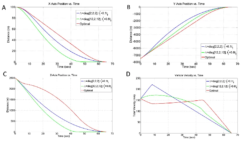
Figure 1. Comparison of MSSG System Trajectories to Optimal Solution

The open-loop, fuel-optimal landing problem is solved assuming that the lander’s initial position and velocity are ( ) [ ] and ( ) [ ] , respectively. The guidance reference frame is fixed to the lunar surface with the origin located at the targeted landing point. The desired final state of the vehicle is set to be ( ) [ ] and ( ) [ ] . The lander is assumed to be a small robotic vehicle, with six throttlable engines, one pointing in each direction ( ). For these simulations, the only dynamical force included is the gravitational force of the moon, as seen in Eq. (42). The lander is assumed to weigh 1900 kg (wet mass) and is capable of a maximum (allowable) thrust of 15 kN as well as a minimum (allowable) thrust of 1.5 N. While this lower thrust limit may not be truly realistic, it provides an extremely idealistic optimal case with which we can compare to the MSSG trajectories. The terminal position is set to be at the origin of the guidance reference frame to be achieved with zero velocity (soft landing). For comparison, the MSSG algorithm is initiated at the same initial conditions and defined to target the same terminal state. Figure 1 shows the trajectories and total velocity histories for the open-loop, fuel-optimal landing guidance found via GPOPS and two MSSG-guided cases. GPOPS found a total optimal flight time equal to

which is also assumed to be the employed by the MSSG guidance scheme. The

optimal case. The fuel-efficient thrust profile is extremal, i.e. the optimal algorithm thrusts at a maximum value until it switches to the minimum allowable thrust, and finally returns to the maximum value (bang-bang type). The MSSG algorithms reduce the thrust command until the second surface is reached. At , the thrust command experiences a large shift and then decreases monotonically until the first surface is achieved. The thrust spike can be in principle reduced by increasing .

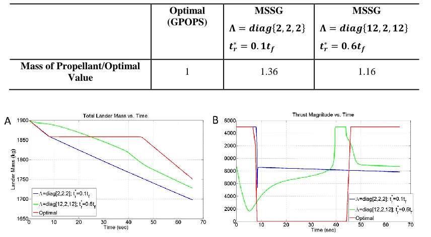
Table 1. Comparison Between the Open-Loop Fuel-Optimal Guidance and the MSSG Guidance (Propellant Mass)

Optimal (GPOPS)

MSSG

{ }

MSSG

{ }

Mass of Propellant/Optimal

Value 1 1.36 1.16

Figure 2. A) Lander Mass and B) Thrust Magnitude Histories Comparing Optimal Solution to MSSG

Clearly, MSSG is sub-optimal. Indeed, in order to better characterize the performance and to find the optimal guidance gains for MSSG, reinforcement learning is implemented. By using reinforcement learning policies to determine a set of optimal guidance gains, the performance of MSSG can truly be optimized in terms of both fuel optimality and landing accuracy.

Parameter Optimization via Reinforcement Learning

In order to explore the potential optimality of the MSSG algorithm, reinforcement learning has been employed to determine an optimal set of guidance gains. The vehicle state [ ] at the start of the powered descent phase (i.e. ) is used for the policy optimization for this particular application and the parameters that were to be learned by this technique are the guidance parameters ( ), the final time of the descent , and the time of convergence of the second sliding surface, . Indeed, these parameters make up the five-dimensional action space for this problem. By utilizing the initial vehicle state, a set of these five parameters was chosen and used for the entirety of that scenario, i.e. only one set of parameters are used and the parameters do not update adaptively during the course of the simulation.

range of starting condition and also account for sensor or navigation errors. By including these in the learning process, the resulting parameters will not only provide optimality from a fuel consumption standpoint, they will also include robustness to initial state perturbations and sensor errors, which is not accounted for in the given optimal trajectory seen in Fig. 1 and 2. The reinforcement learning simulation used to calculate the utility of a certain combination of parameters uses conditions which are very similar to those provided in the previous section. The initial wet mass of the spacecraft remains 1900 kg. The initial conditions of the simulation used to learn the parameters are distributed deterministically according to the values in Table 2. Each of these values are uniformly distributed between the respective minimum and maximum values, providing a total of 144 samples that are used to learn an optimal set of parameters. Further, these simulations included uncertainties of and in position and velocity, respectively, which are provided to the guidance algorithm to simulate sensor noise when estimating the current state of the spacecraft. Finally, the utility function, which is determined at the end of the simulation of each sample, which is used in order to determine which set of parameters is optimal, was chosen to be:

( ) _{‖ ‖ ‖ ‖ ( ) (48)}

Here, the terms ‖ ‖ and ‖ ‖ represent the final position and velocity errors that result from the chosen guidance parameters, represents the difference between the final lander mass resulting from the chosen parameters and the final mass observed from the optimal solution, and and represent weights for each of their respective terms. Essentially, this utility function is attempting to minimize the residual error of the guidance law and minimizing the fuel usage over the given set of initial conditions.

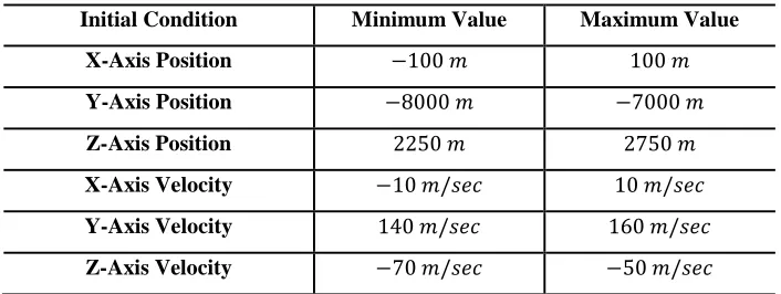
Table 2. Deterministic Initial Conditions for Reinforcement Learning Parameter Optimization

Initial Condition Minimum Value Maximum Value

X-Axis Position

Y-Axis Position

Z-Axis Position

X-Axis Velocity

Y-Axis Velocity

Z-Axis Velocity

The results of this optimization are captured in Table 3. Importantly, the final time of the simulation determined by reinforcement learning is very similar to the value determined by the optimal solution, .

Table 3. Optimal Parameter Results of Reinforcement Learning

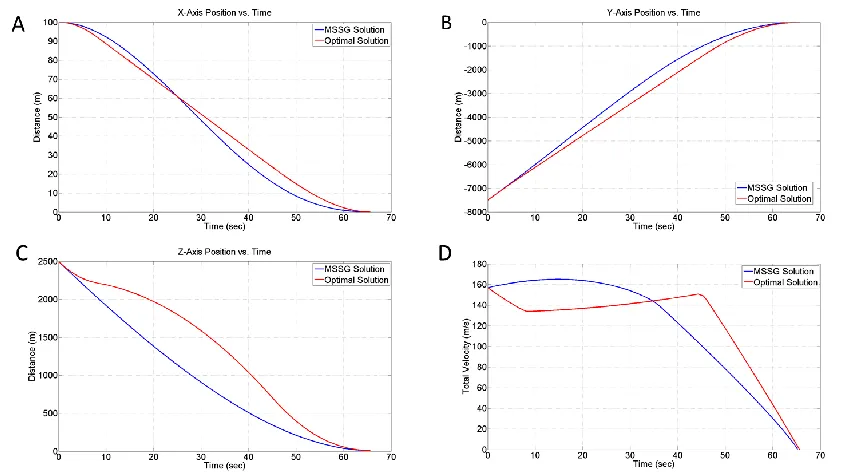
Figure 3. Comparison of Reinforcement Learning Optimized MSSG System Trajectories to Optimal Solution

Figure 4. A) Thrust Magnitude and B) Lander Mass Histories Comparing Optimal Solution to Reinforcement Learning Optimized MSSG

deterministic solution, providing the possibility of retargeting and optimization about off-nominal conditions.

Table 4. Comparison Between the Open-Loop Fuel-Optimal Guidance and the Reinforcement Learning Optimized MSSG Guidance (Propellant Mass)

Optimal (GPOPS)

RL Optimized MSSG

Mass of Propellant/Optimal

Value 1 1.032

Mass of Propellant

Monte Carlo Analysis of Optimized MSSG

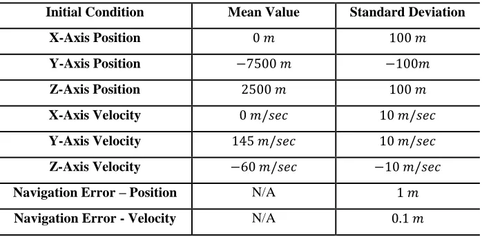
In order to further validate and analyze the robustness and optimality of the learned MSSG parameters, a Monte Carlo analysis has been performed to test the system under off-nominal conditions. The Monte Carlo analysis has been conducted by running 1000 simulations of the MSSG algorithm in the described 3-DOF framework. Table 5 shows the parameters used in the simulations, as well as their dispersions. All values are assumed to follow a normal (Gaussian) distribution described by their respective means and standard deviations. The MSSG parameters and gains are exactly those described in Table 3 and are the result of the Reinforcement Learning optimization. The nominal case for the Monte Carlo simulation is the same as seen in the previous analysis. Further, for each thruster firing, the mass-flow rate is perturbed using a normal distribution which is set assuming an upper value of 10% deviation from the mean value.

Table 5. Initial Condition Dispersions for Monte Carlo Simulation

Initial Condition Mean Value Standard Deviation

X-Axis Position

Y-Axis Position

Z-Axis Position

X-Axis Velocity

Y-Axis Velocity

Z-Axis Velocity

Navigation Error – Position N/A

Figure 5. Monte Carlo Simulation Results: A) X-Axis Position; B) Y-Axis Position; C) Z-Axis Position; and D) Final Landing Location Dispersion

Figure 6. Monte Carlo Simulation Results: A) X-Axis Velocity; B) Y-Axis Velocity; C) Z-Axis Velocity; and D) Velocity Magnitude

nominal conditions. Figures 7 and 8 shows that the residual errors in position and velocity are very near zero. The results of the Monte Carlo simulation are gathered in Table 6.

Figure 7. Monte Carlo Simulation Results: A) X-Axis Miss Distance; B) Y-Axis Miss Distance; and C) Magnitude of Miss Distance

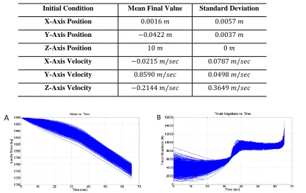
Table 6. Monte Carlo Simulation Result Statistics

Initial Condition Mean Final Value Standard Deviation

X-Axis Position

Y-Axis Position

Z-Axis Position

X-Axis Velocity

Y-Axis Velocity

Z-Axis Velocity

Figure 9. Monte Carlo Simulation Results: A) Lander Mass History; and B) Thrust Magnitude History

Clearly the performance of the algorithm with the given parameters is quite good. Figure 5d shows that the final miss distance is very near zero for all cases, demonstrating the accuracy of the algorithm with the optimized parameters. However, as can be seen in Fig. 8, and Table 6, some cases did contain significant residual velocity error. The residual final velocity has a maximum value of , which is mostly in the direction, as seen in Fig. 8c. However, most of the cases exhibit residual velocity errors much smaller than this. Further, this error can be attributed in part due to the amount of training that was performed within the reinforcement learning environment, and also that the MSSG parameters were determined for the nominal initial condition as opposed to a set of parameters that work best over the entire space defining all possible initial conditions. It is likely that this case was very near the edge of the design space that was used in the learning environment, and as such further training will likely remove these errors.

CONCLUSIONS

them in terms of fuel consumption. Indeed, the results of the reinforcement learning process has provided a set of parameters that bring the performance of the MSSG algorithm very close to that provided by an optimal open-loop solution. Further, the solution does not require the generation of a reference trajectory, and as such is more flexible under off-nominal conditions and perturbations. The features of accuracy, flexibility, and good fuel usage make the MSSG algorithm very applicable for future lunar missions.

Future work for the MSSG algorithm include a) inclusion of additional constraints in the reinforcement learning process, including guide-slope constraints, b) shifting the paradigm of one set of guidance parameters to that of a more adaptive approach, which will allow the reinforcement learning algorithm to learn an optimal set of guidance parameters that update during the descent phase, and c) the application of reinforcement learning of the MSSG algorithm to other scenarios, including asteroid proximity operations and Mars hypersonic reentry and terminal powered landing guidance. These additional features and analysis will allow the MSSG algorithm to be further refined and analyzed under more strenuous conditions and provide further understanding into the true application of the algorithm for future mission architectures.

REFERENCES

1

A. A. Wolf, J. Tooley, S. Ploen, M. Ivanov, B. Acikmese, K. Gromov, Performance Trades for Mars Pinpoint Landing, IEEE Aerospace Conference Proceedings, March 2006, IEEE-1661, March 2006.

2

A. Wolf, E. Sklyanskly, J. Tooley, B. Rush, Mars Pinpoint Landing Systems Trades, AAS/AIAA Astrodynamics Specialist Conference Proceedings, AAS 07-310, August 19-23, 2007

3 _{Phinney, W.C., Criswell, D., Drexler, E., Garmirian, J. “Lunar Resources and Their Utilization”,}

Space-Based Manufacturing from Nonterrestial Materials, AIAA p. 97-123, 1977.

4

A. D., Steltzner, D. M., Kipp, A., Chen, P. D.,Burkhart, C. S., Guernsey, G. F., Mendeck, R. A., Mitcheltree, R. W., Powell, T. P., Rivellini, A. M., San Martin, D. W., Way, Mars Science Laboratory Entry, Descent, and Landing System, IEEE Aerospace Conference Paper No. 2006-1497, Big Sky, MT,(2006).

5

A. R., Klumpp, A Manually Retargeted Automatic Landing System for the Lunar Module (LM), Journal of Spacecraft and Rockets, Volume 5, Issue 2, 1968, pp 129-138.

6

A. R., Klumpp, Apollo Guidance, Navigation, and Control: Apollo Lunar-Descent Guidance, Massachusetts Inst. of Technology, Charles Stark Draper Lab., TR R-695, Cambridge, MA, June 1971.

7

A. R., Klumpp, Apollo Lunar Descent Guidance, Automatica, Volume 10, Issue 2, 1974, pp. 133-146.

8

G. Singh, A. SanMartin, and E. Wong. Guidance and control design for powered descent and landing on Mars.

Aereospace Conference IEEE, 2007.

9 _{U., Topcu, J., Casoliva, and K., Mease, Fuel Efficient Powered Descent Guidance for Mars Landing, AIAA Paper}

2005-6286, 2005.

10

F., Najson, and K., Mease, A Computationally Non-Expensive Guidance Algorithm for Fuel Efficient Soft Landing, AIAA Guidance, Navigation, and Control Conference, San Francisco, AIAAPaper 2005-6289, 2005.

11 _{B., Acikmese, and S. R., Ploen, Convex Programming Approach to Powered Descent Guidance for Mars}

Landing, Journal of Guidance, Control, and Dynamics, Vol. 30, No. 5, 2007, pp. 1353–1366.

12 _{C. D’Souza, An Optimal Guidance Law for Planetary Landing, AIAA Guidance, Navigation, and Control}

Conference, AIAA Paper 1997-3709, 1997.

13

D. A., Benson, G. T., Huntington, T. P., Thorvaldsen, and A. V., Rao, Direct trajectory optimization and costate estimation via an orthogonal collocation method. Journal of Guidance, Control, and Dynamics, 29(6), 2006, 1435-1440.

14

15

B. Acıkmese and L. Blackmore. Lossless convexification of a class of optimal control problems with non-convex control constraints. Automatica, 47(2), 2011.

16

Y., Nesterov, and A., Nemirovsky, Interior-Point Polynomial Methods in Convex Programming, SIAM, Philadelphia, PA, 1994.

17

L. Blackmore, B. Acıkmese, and D. P Scharf. Minimum landing error powered descent guidance for Mars landing using convex optimization. AIAA Journal of Guidance, Control and Dynamics, 33(4):1161–1171, 2010.

18

A., Levant, Construction Principles of 2-Sliding Mode Design, Automatica, Vol. 43, No. 4, (2007), pp. 576–586.

19

Levant, A., Sliding order and sliding accuracy in sliding mode control. International Journal of Control, 58(6), 1993, 1247–1263.

20

A. Levant, Higher-order sliding modes, differentiation and output feedback control. International Journal of Control, 76(9/10), (2003), 924–941.

21

Levant, A. Homogeneity approach to high-order sliding mode design. Automatica, 41(5), (2005a). 823–830.

22

Levant, A., Quasi-continuous high-order sliding-mode controllers. IEEE Transactions on Automatic Control,

50(11), (2005b), 1812–1816.

23

Y. B., Shtessel, & I. A., Shkolnikov, Aeronautical and space vehicle control in dynamic sliding manifolds. International Journal of Control, 76(9/10), 1000–1017, 2003.

24 _{M., U., Salamci, M., K., Ozgoren, S., P., Banks, Sliding Mode Control with Optimal Sliding Surfaces for Missile}

Autopilot Design, Journal of Guidance, Control and Dynamics, Vol. 23, No. 4, 2000.

25 _{Y., Shtessel, and C., Tournes, Integrated Higher-Order Sliding Mode Guidance and Autopilot for Dual-Control}

Missiles, Journal of Guidance, Control and Dynamics, Vol. 32, No. 1, 2009.

26

C., Tournes, Y., Shtessel, I., Shkolnikov, Missile Controlled by Lift and Divert Thrusters Using Nonlinear Dynamic Sliding Manifolds, Journal of Guidance, Control and Dynamics, Vol. 29, No. 3, 2006.

27

A., Koren, M., Idan, O., M., Golan, Integrated Mode Guidance and Control for a Missile with On-Off Actuators,

Journal of Guidance, Control and Dynamics, Vol. 31, No. 1, 2008.

28

R. Furfaro, S. Selnick, M. L. Cupples and M. W. Cribb, Non-Linear Sliding Guidance Algorithms for Precision Lunar Landing, in Advances in the Astronautical Sciences, Volume 140, Proceedings of the 21st AAS/AIAA Space Flight Mechanics Meeting held February 13-17, 2011, New Orleans, Louisiana.

29

R. Furfaro and Daniel R. Wibben, Asteroid Precision Landing Via Multiple Sliding Surfaces Guidance Techniques, Proceedings of the annual AAS/AIAA Astrodynamics Specialists Conference, AAS 11-647, July 31- August 4, 2011, Girdwood, Alaska.

30

R. Furfaro, D. O., Cersosimo and J. Bellerose, Close Proximity Asteroid Operations using Sliding Control Modes, Proceedings of the annual AAS/AIAA Space Flight Mechanics Conference, AAS 12-132, Jan 31-Feb 4, 2012, Charleston, Louisiana.

31 _{N., Harl, and S., N., Balakrishnan, Reentry Terminal Guidance Through Sliding Control Mode, Journal of}

Guidance, Control and Dynamics, Vol. 33, No. 1, January–February 2010.

32

Slotine, J., and Li, W., Applied Nonlinear Control, Prentice Hall, 1991.

33

A. V., Rao, D. A., Benson, C., Darby, M. A., Patterson, C., Francolin, I., Sanders, et al. Algorithm 902: GPOPS, a MATLAB software for solving multiple phase optimal control problems using the Gauss pseudospectral method. ACM Transactions on Mathematical Software, 37(2), 2010, 22:1-22:39.

34 _{P.E. Gill, M.A. Saunders, and W. Murray. SNOPT: An SQP algorithm for large scale constrained optimization.}