Stability of a Class of Delayed Port-Hamiltonian Systems with Application to Droop-Controlled Microgrids

(1)

This is a repository copy of

Stability of a Class of Delayed Port-Hamiltonian Systems with

Application to Droop-Controlled Microgrids

.

White Rose Research Online URL for this paper:

http://eprints.whiterose.ac.uk/92377/

Version: Accepted Version

Proceedings Paper:

Schiffer, JF, Fridman, E and Ortega, R (2015) Stability of a Class of Delayed

Port-Hamiltonian Systems with Application to Droop-Controlled Microgrids. In: IEEE

Conference on Decision and Control. 54th Annual Conference on Decision and Control,

15-18 Dec 2015, Osaka, Japan. Institute of Electrical and Electronics Engineers (IEEE) .

ISBN 978-1-4799-7884-7

https://doi.org/10.1109/CDC.2015.7403226

[email protected] https://eprints.whiterose.ac.uk/ Reuse

Unless indicated otherwise, fulltext items are protected by copyright with all rights reserved. The copyright exception in section 29 of the Copyright, Designs and Patents Act 1988 allows the making of a single copy solely for the purpose of non-commercial research or private study within the limits of fair dealing. The publisher or other rights-holder may allow further reproduction and re-use of this version - refer to the White Rose Research Online record for this item. Where records identify the publisher as the copyright holder, users can verify any specific terms of use on the publisher’s website.

Takedown

If you consider content in White Rose Research Online to be in breach of UK law, please notify us by

(2)

Stability of a class of delayed port-Hamiltonian systems with application to

droop-controlled microgrids

Johannes Schiffer, Emilia Fridman, Romeo Ortega

Abstract— A class of port-Hamiltonian systems with delayed interconnection matrices is considered. This class of systems is motivated by the problem of stability in droop-controlled microgrids with delays. Delay-dependent stability conditions are derived via the Lyapunov-Krasovskii method. The stability conditions are applied to an exemplary microgrid. The efficiency of the results is illustrated via a simulation example.

I. INTRODUCTION

Time delays are a non-negligible phenomenon in many engineering applications, such as networked control systems, biological systems or chemical processes [1]. In particular, the presence of time delays does often have a significant impact on stability properties of equilibria of a system. Hence, guaranteeing robustness with respect to time delays is of paramount importance in a large variety of applications. The main motivation for the present work is the analysis of the effect of time delays on the operation of microgrids (µGs). The µG is an emerging concept in the context of electrical networks with large shares of renewable distributed generation (DG) units [2].µGs have been identified as a key component in future power systems [2]. In short, a µG is a locally controllable subset of a larger electrical grid and is composed of several DG units, storage devices and loads [2]. A key feature of such grids is that they can be operated either in grid-connected or in islanded mode. The latter operation mode increases the reliability of power supply, as it permits to run theµG completely isolated from the main power system. In conventional power systems, most generation units are interfaced to the grid via synchronous generators (SGs). In contrast, most renewable DG units are connected to the network via AC inverters. The latter are power electronic devices, which possess significantly different physical proper-ties from SGs [3]. Hence, new control schemes for networks with large shares of inverter-interfaced units are required [3]. A widely-promoted control scheme to operate inverter-interfaced DG units in µGs is droop control [4]. This is a decentralized proportional control, the main objectives of which are stability and power sharing. For stability analysis of droop-controlled µGs, it is customary to model inverter-interfaced DG units as ideal controllable voltage sources. With this model conditions for stability of droop-controlled µGs have been derived, e.g., in [5]–[7].

J. Schiffer is with Technische Universit¨at Berlin, Germany,

[email protected]

E. Fridman is with Tel-Aviv University, Israel

[email protected]

R. Ortega is with Laboratoire des Signaux et Systémes, Ecole´ Supérieure d’Electricité (SUPELEC), Gif-sur-Yvette 91192, France,

[email protected]

This work was partially supported by the Israel Science Foundation (grant no. 1128/14).

In a practical setup, the droop control scheme is applied to an inverter by means of digital discrete time control. Digital control usually introduces additional effects such as clock drifts [8] and time delays [9], [10], which may have a deteriorating impact on the system performance. According to [10], the main reasons for the appearance of time delays are 1) sampling of control variables, 2) calculation time of the digital controller and 3) generation of the pulse-width-modulation (PWM) to determine the switching signals for the inverter. This fact has not been considered in the previous work [5]–[7] and in [11] only for the special case of aµG composed of two inverters. We refer the reader to, e.g., [10] for further details.

With regards to clock drifts, it is shown in [8] that stability of droop-controlledµGs is robust with respect to constant un-known clock drifts. Therefore, this phenomenon is neglected in the present paper. Instead, we focus on the impact of time delays on stability of droop-controlledµGs. To this end, and following our previous work [6], we represent the µG as a port-Hamiltonian (pH) system with delays. The main advantage of a pH representation is that the Hamiltonian usually is a natural candidate Lyapunov function.

Stability analysis of pH systems with delays has been subject of previous research [12]–[15]. The main motivation of the aforementioned work is a scenario in which several pH systems are interconnected via feedback paths which exhibit a delay. This setup yields a closed-loop system with skew-symmetric interconnections, which can be split into non-delayed skew-symmetric and delayed skew-symmetric interconnections. However, the model of a droop-controlled µG with delays derived in this work is not comprised in the class of pH systems studied in [12]–[15], since the delays do not appear skew-symmetrically. In that regard, the class of systems considered in the present work generalizes the class studied in [12]–[15], see Section III for further details. Moreover, compared to [12], [14], [15], we focus on stability in the presence of fast-varying delays, typically arising in the context of digital control [16], [17].

In summary, the main contributions of the present paper are

(i)to introduce a model of a droop-controlledµG, in which the inverters exhibit an input delay,(ii)to represent this µG model as a pH system with delays,(iii) to provide stability conditions for a class of pH systems with fast-varying delays via the Lyapunov-Krasovskii (LK) method, (iv)to illustrate the utility of the derived conditions on an exemplaryµG.

(3)

Notation. We define the setsn¯ :={1,2, . . . , n}, R_≥₀ _:= {x ∈ R_|_x _≥ _0}_, R_>₀ _:= _{_x _∈ R_|_{x >} _0}_, R_<₀ _:= _{_x _∈ R_|_{x <}_0}_,Z_≥₀_:=_{0_,₁_,₂_{, . . .}_}_andS_{:= [0}_,₂_π₎_{. For a set}_V_,

let|V|denote its cardinality. For a set of, possibly unordered, positive natural numbers V = {l, k, . . . , n}, the short-hand i ∼ V denotes i = l, k, . . . , n. Let x := col(xi) ∈ Rn

denote a vector with entries xi for i ∼ n,¯ 0n the zero

vector, 1n the vector with all entries equal to one, In the

n×nidentity matrix,0n×nthen×nmatrix with all entries

equal to zero and diag(ai), i∼n,¯ ann×ndiagonal matrix

with diagonal entries ai ∈ R. Likewise, A = blkdiag(Ai)

denotes a block-diagonal matrix with matrix entriesAi. We

employ the notation In×mn =

In, . . . , In

∈ Rn×mn_. _Let

x ∈ Rn_, _then _k_x_k _{denotes an arbitrary vector norm. For}

A ∈ Rn×n_{, A >} ₀ _{means that} _A _{is symmetric positive}

definite. The lower-diagonal elements of a symmetric matrix are denoted by ∗. We denote by C[−h,0] the space of continuous functionsφ: [−h,0]→Rn_. _For_x_:_R

≥0→Rn,

we denotext(σi) =x(t+σi), σi∈[−h,0].Also,∇f denotes

the transpose of the gradient of a functionf :Rn _→_R_,_∇2_H

its Hessian matrix, we employ the notation∇f˙=d(∇f)/dt and iff takes the form f =f(x(t−h)), x∈Rn_, _{we use}

the short-hand ∇fh=∇f(x(t−h)).

II. MOTIVATING APPLICATION:DROOP-CONTROLLED

µGS WITH HETEROGENEOUS DELAYS

A. Network model

We consider a Kron-reduced [19] generic inverter-based µG in which loads are modeled by constant impedances. The network is composed of n ≥ 1 inverters and the set of network nodes is denoted by n.¯ As done in [5], [6], we assume that the line admittances are purely inductive. Then, two nodesiandkin the network are connected by a nonzero susceptanceBik∈R<0.The set of neighbors of thei-th node

is denoted byn¯i={k∈n¯|Bik6= 0}.We associate a

time-dependent phase angleδi :R≥0→Sto each nodei∈n¯ and

use the common short-handδik:=δi−δk, i∈n, k¯ ∈n.¯

Also, we make the frequent assumption, see, e.g., [5], that the voltage amplitudes Vi ∈ R>0 at all nodes i ∈ n¯ are

constant. Then, the active power injection Pi : Sn → R of

thei-th inverter is given by [19]1 Pi(δ1, . . . , δn) =GiiVi2+

X

i∼n¯i

aiksin(δik), (II.1)

where aik = |Bik|ViVk > 0 and Gii ∈ R≥0 denotes the

shunt conductance at thei-th node.

Finally, we assume that the µG is connected, i.e., that for all pairs (i, k) ∈ n¯ × n, i¯ 6= k, there exists an ordered sequence of nodes from i to k such that any pair of consecutive nodes in the sequence is connected by a power line represented by an admittance. This assumption is reasonable for aµG, unless severe line outages separating the system into several disconnected parts occur.

B. Inverter model with input delay

As outlined in Section I, inverter-based DG units usually exhibit an input delay originating from the fact that they are

1_{To simplify notation the time argument of all signals is omitted, whenever}

clear from the context.

controlled via digital discrete time control [10]. In general, not all inverters in aµG are identical with respect to their hardware and the implementation of the digital controls. Consequently, the delays are, in general, heterogeneous.

The delay induced by the digital control is typically composed of two main parts: a constant delay η ∈ R_>₀

originating from the calculation time of the control signal2 and the PWM and an additional delay caused by the sample-and-hold function of control variables [10]. Following [1], [16], we assume that the sampling intervals are bounded, i.e.,tκ+1−tκ≤hs, κ∈Z≥0.Then,

tκ+1−tκ+η≤hs+η := ¯h, (II.2)

where¯hdenotes the maximum time interval between the time tκ−η,where the measurement is sampled and the timetκ+1,

where the next control input update arrives.

With these considerations, by following [1], [16] and the usual modeling of inverters, see [8], the inverter at the i-th node with input delay and zero-order-hold update characteristic with sampling instantsti,κ,can be represented

by3

˙

δi(t) =uδi(ti,κ−ηi),

τPiP˙ m

i (t) =−Pim(t) +Pi(t),

ti,κ≤t < ti,κ+1, κ∈Z≥0,

(II.3)

whereuδ

i : R≥0 → R is the control input, ηi ∈ R>0 is a

constant delay,Pi is given by (II.1), Pim:R≥0 →Ris the

measured active power and τPi ∈R>0 is the time constant

of the measurement filter. We assume that the inverters are controlled via the usual frequency droop control given by [4]

uδ

i(t) =ωd−kPi(P

m₍_t₎₋_Pd

i). (II.4)

C. Closed-loop droop-controlledµG

As shown in [1], [16], the type of delay appearing in the open-loop system (II.3) results in a fast-varying delay, once the loop is closed. To see this, definehi(t) :=t−ti,κ+ηi,

ti,κ≤t < ti,κ+1.Then, combining (II.3) with (II.4), yields

the closed-loop system

˙

δi(t) =ωd−kPi(P

m₍_t₋_h

i(t))−Pid),

τPiP˙ m

i (t) =−Pim(t) +Pi(t).

(II.5)

Note that (II.2) implies thatηi≤hi(t)≤ti,κ+1−ti,κ+ηi≤ ¯

hi andh˙i(t) = 1. Via the affine state transformation [6]

δi

ωi

=

1 0 0 −kPi

δi

Pm i

+

0 0 0 1

0

ωd₊_k PiP

d i

,

the system (II.5), (II.4) can be written as

˙

δi(t) =ωi(t−hi(t)),

τPiω˙i(t) =−ωi(t) +ω d₋_k

Pi Pi(t))−P d i

. (II.6) It is convenient to introduce the notion of a desired synchronized motion.

2_{Note that the delay}_η _{may also represent the dynamics of the internal}

control system of the inverter, which is not considered explicitly in the model (II.5). See [20] for a detailed model derivation of the non-delayed version of (II.5).

3_{An underlying assumption to this model is that whenever the inverter}

(4)

Definition 2.1: A solution col(δs_{, ω}s₁

n)∈Sn×Rn of the

system (II.1), (II.6),i∼¯n,is a desired synchronized motion ifωs_∈_R

>0 is constant andδs∈Θ, where

Θ :=nδ∈Sn|δik|<

π

2, i∼n, k¯ ∼n¯i

o ,

such thatδs

ik=δsi−δsk are constant,i∼n, k¯ ∼n¯i,∀t≥0.

Note that along any synchronized motion,

X

i∼¯n ˙

ωi= 0 ⇒ ωs=ωd+

P

i∼n¯ Pid−GiiVi2

P

i∼n¯ 1

kPi

,

i.e., for each choice of parameters kPi and P d

i, the system

(II.1), (II.6), i ∼ n,¯ possesses a unique synchronization frequency, see [5], [6]. We make the following natural power-balance feasibility assumption, see [6].

Assumption 2.2: The system (II.1), (II.6),i∼n,¯ possesses a desired synchronized motion.

We denote the vector of phase angles byδ=col(δi)∈Sn

and the vector of frequenciesωi= ˙δi byω=col(ωi)∈Rn.

Under Assumption 2.2, we introduce the error states

˜

ω(t) :=ω(t)−ωs₁

n∈Rn,δ˜(t) :=δ(0)−δs(0)+

Z t

0

˜

ω(τ)dτ∈Rn_.

Furthermore, by noting that the power flows (II.1) only depend upon angle differences, we express all angles relative to an arbitrarily chosen reference node, say noden, i.e.,

θ:=Cδ,˜ C:=

I(n−1) −1(n−1)

.

For ease of notation, we define the constantθn := 0, which

is not part of the vectorθ.In the reduced angle coordinates, the power flows (II.1) become

Pi(˜δ(θ)) =

X

k∼nˆi

aiksin(θik+δiks). (II.7)

By introducingc1:=col(c1i)∈Rn, c1i:=ω

d₋_ωs₊_k PiP

d i,

as well as the matrices KP = diag(kPi) ∈ Rn×n, TP =

diag(τPi)∈Rn×n,the error dynamics of (II.6), (II.7),i∼n,¯

are given in the coordinatesx:=col(θ,ω˜)∈R(n−1)_×_Rn _by ˙

θ(t) =Cω˜h,

TPω˙˜(t) =−˜ω(t)−KPP(˜δ(θ)) +c1,

(II.8)

whereω˜h :=col(˜ωi(t−hi))∈C[−h,0]n, h= maxi∼n¯¯hi

and P(˜δ(θ)) =col(Pi(˜δ(θ))) ∈Rn with Pi(˜δ(θ))given in

(II.1). Note that the system (II.8) possesses an equilibrium pointxs_{= 0}

2n−1, the asymptotic stability of which implies

asymptotic convergence of all trajectories of the system (II.6), (II.7), i ∼n,¯ to the synchronized motion (up to a uniform shift of all angles).

We are interested in the following problem.

Problem 2.3: Consider the system (II.6), (II.7),i∼n¯with Assumption 2.2. Given ¯hi, i ∼ n,¯ derive conditions, such

that the corresponding equilibrium point of (II.8) is (locally) asymptotically stable.

Note that it follows from Proposition 5.9 in [6] that with Assumption 2.2 and forhi= 0, i∼¯n,i.e., the non-delayed

version of (II.8), the equilibrium pointxs_{= 0}

2n−1is locally

asymptotically stable for any choice ofTP, KP andPd.

III. ACLASS OF PHSYSTEMS WITH DELAYS

To address Problem 2.3 and by following the analysis in [6], we note that withx=col(θ,ω˜)∈Rn−1_×Rn _{the system}

(II.8) can be written as a perturbed pH system with delays

˙

x= (J − R)∇H+X i∼n¯

Ti(∇Hhi− ∇H), (III.1)

with HamiltonianH :R(n−1)_×_Rn_→_R

H(x) = n

X

i=1

τ_P

i 2kPi

˜

ω2_i−1 2

X

k∼n¯i

aikcos(θik+δiks)

− n−1

X

i=1

c1i

kPi

θi,

(III.2) interconnection matrix

J =

"

0(n−1)×(n−1) CKPTP−1 − CKPTP−1

⊤

0n×n

#

,

damping matrix R = diag(0(n−1), KP(T_P−2)1n) and Ti = JMi,whereMi∈R(2n−1)×(2n−1),the(n−1+i, n−1+i)

-th entry ofMi is one and all its other entries are zero.

Given this fact, it seems natural to analyze (II.8) by exploiting its pH structure (III.1). Hence, for our analysis, we consider a generic nonlinear time-delay system in perturbed Hamiltonian form

˙

x= (J(x)− R(x))∇H+ m

X

i=1

(Ti(∇Hhi− ∇H)), (III.3)

with state vectorx:R_≥₀_→Rn_{, m >}₀ _delays_h

i:R≥0→

R_>₀_{, h}_i₍_t₎ _∈ _[0_,¯_h_i_]_, ¯_h_i _∈ R_≥₀_, _h˙_i₍_t_{) = 1}_, _Hamiltonian

H :Rn _→R_,_matrices_J₍_x_{) =}_−J₍_x₎⊤ _∈Rn×n_, _R(_x₎_≥ 0∈Rn×n_, _{the entries of which depend smoothly on}_x,_and Ti∈Rn×n, i= 1, . . . m.

In [12]–[15], stability conditions have been derived for pH systems with time delays of the form

˙

x= (J(x)− R(x))∇H+ m

X

i=1

Ti∇Hhi, (III.4)

where Ti are arbitrary interconnection matrices and hi are

time-varying delays. It is easily verified that the system (II.8) cannot be written in the form (III.4). Furthermore, the class of systems (III.4) is a special case of the class (III.3) considered in this paper. To see this, consider two pH systems

˙

x1= (J1(x1)− R1)∇H1+ζ1u1, y1=ζ1⊤∇H1,

˙

x2= (J2(x2)− R2)∇H2+ζ2u2, y2=ζ2⊤∇H2

(III.5)

and feedback interconnections

u2=y1(t−h(t)), u1=y2(t−h(t)), (III.6)

where h(t) is a transmission delay (uniform, for ease of presentation). Then, the resulting closed-loop system is of the form (III.3), i.e.,x˙ = (J(x)− R)∇H+T1(∇Hh− ∇H).

In addition, consider a scenario in which the delay appears only in one of the feedback interconnections of (III.6), then the system (III.5), (III.6) also takes the form (III.3).

IV. DELAY-DEPENDENT STABILITY CONDITIONS FOR FAST-VARYING DELAYS

This section is dedicated to the stability analysis of pH systems with bounded fast-varying delays represented by (III.3). The employed approach is based on a strict LK functional. To streamline our main result, we note that

∇H˙ =∇2_H _{(J − R −}

m

X

i=1

Ti)∇H+ m

X

i=1

Ti∇Hhi

(IV.1)

(5)

Assumption 4.1: The system (III.3) possesses an equilib-rium pointxs_{= 0}

n∈Rn.

Assumption 4.2: Consider the system (III.3) with Assump-tion 4.1 and sethi = 0, i∼n.¯ Then, the equilibrium point

xs_{of the system (III.3) is (locally) asymptotically stable with}

Lyapunov functionV1=H.

Our main result is as follows.

Proposition 4.3: Consider the system (III.3) with Assump-tions 4.1 and 4.2. Given h¯i ≥ 0, i = 1, . . . , m, if there

exist n×n matrices Y > 0, Ri > 0, Si > 0 and S12,i,

i= 1, . . . , m,such that 



Φ11 Φ12 Φ13

∗ −S−R R−S⊤ 12

∗ ∗ Φ33



<0, (IV.2)

where

R=blkdiag(Ri), S =blkdiag(Si), S12=blkdiag(S12,i),

W=∇2H(J − R − m

X

i=1

Ti), M=∇2HIn×nm,

B=

T⊤

1 (R1−S12,1) . . . Tm⊤(Rm−S12,m),

Φ11=−R −0.5

m

X

i=1

Ti+ m X i=1 T⊤ i !

+W⊤_Y ₊_Y_W

+ m X i=1 ¯

h2i (TiW)

⊤

Ri(TiW) +Ti⊤(Si−Ri)Ti

,

Φ12=

T⊤

1 S12,1 . . . Tm⊤S12,m

,

Φ13= 0.5In×nm+ Y + m

X

i=1

¯

h2i (TiW)⊤RiTi

!

M+B,

Φ33=blkdiag −2Ri+S12,i+S⊤12,i

+ m X i=1 ¯

h2i(TiM)

⊤

Ri(TiM), (IV.3)

and

R S12

∗ R

≥0 (IV.4)

are feasible in a neighborhood of xs_, _{then the equilibrium}

xs _{is (locally) uniformly asymptotically stable for all}

fast-varying delayshi(t)∈[0,¯hi], i= 1, . . . , m.

Proof: Inspired by [14], [17], [21], leth= maxi∼n¯¯hi

and consider the LK functionalV :C[−h,0]n_→_R_,

V =V1+V2+

m

X

i=1

(V3i+V4i), V1=H,

V2=∇H⊤Y∇H, V3i= ¯hi

Z 0

−¯hi

Z t

t+φ

σi(s)dsdφ,

V4i =

Z t

t−¯hi

(Ti∇H(s))⊤Si(Ti∇H(s))ds,

(IV.5)

where σi(s) = (Ti∇H˙(s))⊤Ri(Ti∇H˙(s)), i = 1, . . . , m.

Under the made assumptionsH is (locally) positive definite around xs _and _∇_H_|

xs = 0

n, which implies that V is

an admissible LK functional for the system (III.3) with equilibrium pointxs_._Let_ζ_∈_R(2m+1)n_,

ζ=col(∇H,T1∇H¯_h

1, ...,Tm∇Hh¯m,T1∇Hh1, ...,Tm∇Hhm).

The time-derivative ofV1is given by

˙

V1=ζ⊤





−R −0.5(T⊤₊_T_{) 0}

n×mn 0.5In×mn ∗ 0mn×mn 0mn×mn ∗ ∗ 0mn×mn



ζ,

whereT =Pm

i=1Ti.With∇H˙ given by (IV.1) andWgiven

in (IV.3), we have that

˙

V2=ζ⊤





W⊤_Y ₊_Y_W ₀

n×mn YM ∗ 0mn×mn 0mn×mn ∗ ∗ 0mn×mn



ζ,

withMgiven in (IV.3). Furthermore,

˙

V3i = ¯h

2

iσi(s)−¯hi

Z t

t−¯hi

σi(s)ds,

where

σi(s) =ζ⊤





(TiW)

⊤

Ri(TiW) 0n×nm (TiW)

⊤

RiTiM ∗ 0nm×nm 0nm×nm ∗ ∗ (TiM)⊤RiTiM



ζ,

withMgiven in (IV.3). By following [17],

−

Z t

t−¯hi

σi(s)ds=−

Z t−hi(t)

t−¯hi

σi(s)ds−

Z t

t−hi(t)

σi(s)ds. (IV.6)

Suppose that the LMI (IV.4) is feasible. Applying Jensen´s inequality together with Lemma 1 in [17], see also [22], to both right hand side terms in (IV.6) yields4

−¯hi

Z t

t−h¯i

σi(s)ds≤ −

ei1 ei2

⊤

Ri S12,i ∗ Ri

ei1 ei2

, i= 1, . . . , m,

withei1 =Ti(∇H− ∇Hhi)andei₂ =Ti(∇Hhi− ∇H¯hi).

Hence,

m

X

i=1

−¯hi

Z t

t−h¯

σi(s)ds

≤

ζ⊤ 



−Pm

i=1(T ⊤

i RiTi) Φ12 B

∗ −R R−S⊤ 12

∗ ∗ −2R+S12+S12⊤



ζ,

whereR, S, S12,BandΦ12are defined in (IV.3). In addition,

˙

V4i = (Ti∇H)

⊤

Si(Ti∇H)− Ti∇H¯_hi

⊤

Si Ti∇H¯_hi

. Consequently, if

˙

V ≤ζ⊤ 



Φ11 Φ12 Φ13

∗ −S−R R−S⊤ 12

∗ ∗ Φ33



ζ,

whereΦ11, Φ12,Φ13 andΦ22 are defined in (IV.3). Clearly,

if (IV.2) is feasible, then V˙ ≤ −εkx(t)k2 _{for some} _{ε >}₀_.

The proof is completed by invoking the LK theorem, see, e.g., Theorem 1 in [17] and arguments from [24] for systems with piecewice-continuous delays.

Remark 4.4: The conditions given in Proposition 4.3 are state-dependent. We note that, in many cases, the conditions can be conveniently implemented numerically via a polytopic approach [1], [15]. This is also the procedure taken in Section V of the present paper to investigate stability of an equilibrium of the system (II.8).

4_Note _that _instead _of _Jensen´s _inequality, _also _Wirtinger´s

inequality [15] could be employed to upper bound the terms

−h¯iR t t₋h¯i(Ti∇

˙

(6)

PCC 110/20 kV Main electrical network

1

2 3

4

8

9 10

11

∼

= PV

∼

= PV _∼

= Wind ∼

= PV

∼

= PV

∼ = Bat ∼

= FC

∼

= PV

∼ = FC CHP ∼

= FC CHP 9a

9b

9c 10a

10b

[image:6.612.72.286.55.167.2]

10c

Fig. 1. Benchmark model adapted from [25] with 6 main buses and inverter– interfaced units of type: PV–Photovoltaic, FC–fuel cell, Bat–battery, FC CHP. PCC denotes the point of common coupling to the main grid. The sign↓denotes loads.

V. NUMERICAL EXAMPLE

Proposition 4.3 is illustrated via a numerical example based on the inner ring of the islanded Subnetwork 1 of the CIGRE benchmark MV distribution network [25]. The network consists of eight main buses and is shown in Fig. 1. We assume that the generation sources at buses 9b, 9c, 10b and 10c are operated with droop control, while the remaining sources are operated in PQ-mode [20]. See [25] or [6] for a detailed discussion of the employed benchmark model. Furthermore, we associate to each inverter a power rating SN _{= [0}_.₅₁₇_,₀_.₃₅₃_,₀_.₃₃₃_,₀_._023]_{pu, where pu denotes per}

unit values with respect to the base power Sbase= 3 MVA. Following Lemma 6.2 in [6], we select Pd

i = 0.6SiN pu

and kPi = 0.2/S N

i Hz/pu, i ∼ n.¯ The low pass filter time

constants are set toτP = [0.1,0.6,0.8,0.2]s.

A. Estimate of region of attraction of non-delayed system

As the conditions given in Proposition 4.3 are state-dependent, to perform a numerical analysis, it is useful to obtain an estimate of a meaningful region of the state-space in which the conditions of Proposition 4.3 shall be satisfied. Here, we address this issue by deriving an estimate of the region of attraction of the non-delayed version of system (III.1). An extension to the delayed case may be of potential interest and we plan to address this aspect in the future.

Besides, estimating the region of attraction in µGs and power systems is an interesting and challenging problem on its own [18]. In that regard, we remark that the result below is an independent result for the non-delayed model of (III.1).

Lemma 5.1: Consider the system (III.1) with Assump-tion 2.2 and ¯hi = 0, i ∼ n.¯ Fix a small positive number

ϑ, such that |θik+δiks| < π2 −ϑ, i ∼ n, k¯ ∼ ¯ni and an

arbitrarily large positive number β ≫ ϑ. Estimates of the domain of attraction of the asymptotically stable equilibrium pointxs_{= 0}

2n−1 are the sublevel sets

Ωc={x=col(θ,ω˜)∈R(2n−1)|H(x)≤c},

that are contained in

D={x∈R(2n−1)_{| k}_x_{k ≤}_β, |θik+δiks| ≤

π

2 −ϑ, i∼n, k¯ ∼n¯i}.

Proof: Following [26], the claim is established by exploiting properties of sublevel sets of strongly convex closed functions together with the fact that from (III.1) it

follows that

˙

H =−∇H⊤R∇H≤0 ∀x∈R(2n−1)_. _(V.1)

We start by noting that the continuity of H defined in (III.2) together with the fact that D is a closed set implies thatH is a closed function on D,cf. A 3.3 of [27]. Hence, the sublevel sets ofH onDare closed, cf. A 3.3 of [27].

Next, we establish boundedness of the sublevel sets ofH contained in D. To this end, we recall the fact that if H in (III.2) is a strongly convex closed function on some set

Sǫ ⊂R(2n−1), then the sublevel sets of H contained inSǫ

are bounded, cf. Chapter 9 of [27]5. Strong convexity of H on some setSǫ⊂R(2n−1) is equivalent to∇2H ≥ǫI(2n−1)

for some positive realǫ and allx∈ Sǫ,cf. Chapter 9, [27].

ForH given in (III.2), we have that

∇2_H₌

L(θ) 0(n−1)×n ∗ diag(τPi/kPi)

,

where L : R(n−1) _→ _R(n−1)×(n−1) _with _l

ii =

P

k∼n¯aikcos(θik+δiks), lip = −aipcos(θip +δips), i ∼ ¯

n\{n}, p∼n¯\{n}.The image ofLon the compact domain

Dθ := {θ ∈ Rn−1| |θik+δiks| ≤ π

2 −ϑ, i ∼ n, k¯ ∼ ¯ni}

(recall from Section II-C thatθn= 0 is a constant) is given

by the matrix polytope LP ₌ _{L ₌ Pq

i=1αiLi|αi ≥ 0,Pq

i=1αi = 1}, where m ≤ n(n−1)/2 is the number

of angle differences and q = 2m _{the number of vertices} Li of the polytope. Denote the n −1 eigenvalues of a

matrix L ∈ LP _by _λ

k, k = 1, . . . , n−1. It follows from

Lemma 5.8 in [6] that λk > 0, k = 1, . . . , n−1, for any L ∈ LP_. _{Following [28], define the eigenvalue set of the}

matrix polytopeLP _by_Λ(LP_{) :=}_{_λ

k(L), k= 1, . . . , n− 1, L ∈ LP_}_. _{Denote the convex hull of all eigenvalues of}

all vertex matricesLi, i= 1, . . . , q,byconv{λk(Li), k= 1, . . . , n−1, i= 1, . . . , q}.Note that anyLi, i= 1, . . . , q,

is symmetric and, hence, normal. Then, by Theorem 1 in [28], Λ(LP₎ _⊂ _conv_{_λ

k(Li), k = 1, . . . , n−1, i = 1, . . . , q}. Let γ := minλkconv{λk(Li), k = 1, . . . , n− 1, i = 1, . . . , q} > 0. Clearly, there also exists a constant

0 < ǫ < minγ,mini∼¯n

_τ

Pi kPi

, such that ∇2_H _≥

ǫI(2n−1), ∀col(θ,w˜)∈ D. This proves that H is strongly

convex onD,which implies that the sublevel setsΩc={x∈ R(2n−1)_|_H₍_x₎_≤_c_} _{contained in}_D_{are bounded.}

Summarizing, we have shown that the sublevel sets of H contained in D are closed and bounded, hence compact. The proof is completed by noting that (V.1) implies that all sublevel sets ofH contained inDare positively invariant.

B. Stability analysis

We set m = 4 and ¯hi = ¯h ∈ R>0, i ∼ n,¯ in the

numerical analysis, i.e., we assume that all droop-controlled units exhibit a delay with the same upper bound. Furthermore, we recall the setDdefined in Lemma 5.1 and note that for the considered scenario a feasible choice isϑ= 10−8_. _The

numerical implementation of the conditions (IV.2), (IV.4) is done using Yalmip [29]. To this end, we note that in the present case the variables θi only appear as arguments of

the cos-function in condition (IV.2). Therefore, it is fairly

5_{Note that strong convexity is a sufficient, not a necessary condition for}

(7)

0 1 2 3 4 5 6 7 8 9 0.6

0

.7

0

.8

P

/S

N

[-]

0 1 2 3 4 5 6 7 8 9

−3 −2.5

−2 −1.5

·10−2

t[s]

∆

fi

[H

[image:7.612.69.290.50.161.2]

z]

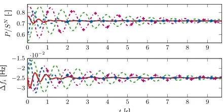
Fig. 2. Simulation example of a droop-controlledµG with fast-varying delays withh¯i= 0.04, i∼n.¯ Trajectories of the power outputs relative to source ratingPi/SiN,and the inverter frequenciesfi= 2πωiin Hz of the controllable sources in theµG. The lines correspond to the following sources: FC CHP 9b,i= 1’–’, FC CHP 9c,i= 2’- -’, battery 10b,i= 3

’+-’ and FC 10c,i= 4’* -’.

straight-forward to adopt a polytopic approach, i.e., to repre-sent the set {∇2_H₍_x₎_|_x_{∈ D}} _as _∇_H2 ₌Pq

i=1αi∇2Hi, 0≤αi ≤1,Pqi=1αi = 1, where∇2Hi denote the vertices

of the polytope containing all instances that∇2_H_{can take on}

the setD,see also the proof of Lemma 5.1. We remark that the region of attraction of the delayed system may, in general, not be identical to D, yet the feasibility of the conditions of Proposition 4.3 for all vertices ∇2_Hi _{together with the}

positive definiteness of the LK functional (IV.5) ensures the existence of a compact positively invariant set for initial conditionsx0 close enough toxsand, thus, local asymptotic

stability of xs_. _{For the considered network, the number of}

nodes in the Kron-reduced network is 4. Hence, we have n(n−1)/2 = 6 angle differences and can describe the set

{∇2_H₍_x₎_|_x_{∈ D}}_with_q_{= 2}6 _{vertices. For the chosen set}

of parameters, the maximal admissible delay is¯h= 0.04.

C. Simulation example

Proposition 4.3 is illustrated via a simulation example. We note that the largest R/X ratio in the Kron-reduced network corresponding to that in Fig. 1 is 0.30. For HV transmission lines it is typically 0.31, see [6]. Thus, the assumption of dominantly inductive admittances is satisfied and the resistive part of the line admittances is neglected in the simulations. The results displayed in Fig. 2 show that the trajectories of the system (II.8) with ¯hi = 0.04,

i ∼ n,¯ converge to a synchronized motion if the sufficient conditions (IV.2), (IV.4) are satisfied. Here, we have assumed constant sampling intervalshi,s = 2·10−4,see (II.2). With ¯

hi = 0.04, the maximum admissible delay in simulation is 1.4¯hi.This indicates that the derived sufficient conditions are

very effective for the system under investigation. We note that the conditions could be further improved by employing more complex LK functionals, e.g., by using ideas from [16], [23].

VI. CONCLUSIONS

Motivated by the problem of stability in droop-controlled inverter-based µGs with delays, we have provided sufficient delay-dependent conditions for stability of a class of pH systems. The conditions are derived via an LK functional and have proven to be effective in a practical example of a µG. Future work will extend the analysis toµGs with inverter- and SG-interfaced DG units, as well as to more detailed inverter and network models. Also, we seek to provide an estimate of the region of attraction ofµGs with delays.

REFERENCES

[1] E. Fridman,Introduction to time-delay systems: analysis and control. Birkh¨auser, 2014.

[2] N. Hatziargyriou, H. Asano, R. Iravani, and C. Marnay, “Microgrids,”

IEEE Power and Energy Magazine, vol. 5, no. 4, pp. 78–94, 2007. [3] T. Green and M. Prodanovic, “Control of inverter-based micro-grids,”

Electric Pow. Sys. Research, vol. Vol. 77, no. 9, pp. 1204–1213, 2007. [4] J. Guerrero, P. Loh, M. Chandorkar, and T. Lee, “Advanced control architectures for intelligent microgrids – part I: Decentralized and hierarchical control,” IEEE Transactions on Industrial Electronics, vol. 60, no. 4, pp. 1254–1262, 2013.

[5] J. W. Simpson-Porco, F. D¨orfler, and F. Bullo, “Synchronization and power sharing for droop-controlled inverters in islanded microgrids,”

Automatica, vol. 49, no. 9, pp. 2603 – 2611, 2013.

[6] J. Schiffer, R. Ortega, A. Astolfi, J. Raisch, and T. Sezi, “Conditions for stability of droop-controlled inverter-based microgrids,”Automatica, vol. 50, no. 10, pp. 2457–2469, 2014.

[7] U. M¨unz and M. Metzger, “Voltage and angle stability reserve of power systems with renewable generation,” in 19th IFAC World Congress, Cape Town, South Africa, 2014, pp. 9075–9080.

[8] J. Schiffer, R. Ortega, C. Hans, and J. Raisch, “Droop-controlled inverter-based microgrids are robust to clock drifts,” inACC, Chicago, IL, USA, 2015, pp. 2341–2346.

[9] D. Maksimovic and R. Zane, “Small-signal discrete-time modeling of digitally controlled PWM converters,” IEEE Transactions on Power Electronics, vol. 22, no. 6, pp. 2552–2556, 2007.

[10] T. Nussbaumer, M. L. Heldwein, G. Gong, S. D. Round, and J. W. Kolar, “Comparison of prediction techniques to compensate time delays caused by digital control of a three-phase buck-type PWM rectifier system,”IEEE Transactions on Industrial Electronics, vol. 55, no. 2, pp. 791–799, 2008.

[11] D. Efimov, R. Ortega, and J. Schiffer, “ISS of multistable systems with delays: application to droop-controlled inverter-based microgrids,” in

ACC, Chicago, IL, USA, 2015, pp. 4664–4669.

[12] R. Pasumarthy and C.-Y. Kao, “On stability of time delay Hamiltonian systems,” inACC, 2009, pp. 4909–4914.

[13] R. Yang and Y. Wang, “Stability analysis for a class of nonlinear time-delay systems via hamiltonian functional method,” in8th World Congress on Intel. Control and Autom. IEEE, 2010, pp. 2874–2879. [14] C.-Y. Kao and R. Pasumarthy, “Stability analysis of interconnected Hamiltonian systems under time delays,”IET control theory & appli-cations, vol. 6, no. 4, pp. 570–577, 2012.

[15] S. Aoues, W. Lombardi, D. Eberard, and A. Seuret, “Robust stability for delayed port-hamiltonian systems using improved wirtinger-based inequality,” inConference on Decision and Control, 2014.

[16] K. Liu and E. Fridman, “Wirtinger’s inequality and Lyapunov-based sampled-data stabilization,”Autom., vol. 48, no. 1, pp. 102–108, 2012. [17] E. Fridman, “Tutorial on Lyapunov-based methods for time-delay systems,”Europ. Jour. of Control, vol. 20, no. 6, pp. 271–283, 2014. [18] U. M¨unz and D. Romeres, “Region of attraction of power systems,” inEstim. and Ctrl. of Networked Syst., vol. 4, no. 1, 2013, pp. 49–54. [19] P. Kundur,Power system stability and control. McGraw-Hill, 1994. [20] J. Schiffer, D. Zonetti, R. Ortega, A. Stankovic, T. Sezi, and J. Raisch,

“Modeling of microgrids—from fundamental physics to phasors and voltage sources,”arXiv preprint arXiv:1505.00136, 2015.

[21] E. Fridman, M. Dambrine, and N. Yeganefar, “On input-to-state stability of systems with time-delay: A matrix inequalities approach,”

Automatica, vol. 44, no. 9, pp. 2364–2369, 2008.

[22] P. Park, J. W. Ko, and C. Jeong, “Reciprocally convex approach to stability of systems with time-varying delays,”Automatica, vol. 47, no. 1, pp. 235–238, 2011.

[23] A. Seuret and F. Gouaisbaut, “Wirtinger-based integral inequality: application to time-delay systems,” Automatica, vol. 49, no. 9, pp. 2860–2866, 2013.

[24] E. Fridman, A. Seuret, and J.-P. Richard, “Robust sampled-data sta-bilization of linear systems: an input delay approach,” Automatica, vol. 40, no. 8, pp. 1441–1446, 2004.

[25] K. Rudion, A. Orths, Z. Styczynski, and K. Strunz, “Design of benchmark of medium voltage distribution network for investigation of DG integration,” inIEEE PESGM, 2006.

[26] M. Galaz, R. Ortega, A. S. Bazanella, and A. M. Stankovic, “An energy-shaping approach to the design of excitation control of syn-chronous generators,”Automatica, vol. 39, no. 1, pp. 111–119, 2003. [27] S. Boyd and L. Vandenberghe, Convex optimization. Cambridge

university press, 2009.

[28] Q.-G. Wang, “Necessary and sufficient conditions for stability of a matrix polytope with normal vertex matrices,” Automatica, vol. 27, no. 5, pp. 887–888, 1991.