White Rose Research Online URL for this paper:
http://eprints.whiterose.ac.uk/85367/
Version: Accepted Version
Proceedings Paper:
Aziz, Furqan, Wilson, Richard C. orcid.org/0000-0001-7265-3033 and Hancock, Edwin R.
orcid.org/0000-0003-4496-2028 (2014) Commute time for a gaussian wave packet on a
graph. In: Structural, Syntactic, and Statistical Pattern Recognition:Joint IAPR International
Workshop, S+SSPR 2014, Joensuu, Finland, August 20-22, 2014. Proceedings. Joint
IAPR International Workshop on Structural, Syntactic, and Statistical Pattern Recognition,
S+SSPR 2014, 20-22 Aug 2014 Lecture Notes in Computer Science (including subseries
Lecture Notes in Artificial Intelligence and Lecture Notes in Bioinformatics) .
Springer-Verlag , pp. 374-383.
https://doi.org/10.1007/978-3-662-44415-3_38
[email protected] https://eprints.whiterose.ac.uk/ Reuse
Items deposited in White Rose Research Online are protected by copyright, with all rights reserved unless indicated otherwise. They may be downloaded and/or printed for private study, or other acts as permitted by national copyright laws. The publisher or other rights holders may allow further reproduction and re-use of the full text version. This is indicated by the licence information on the White Rose Research Online record for the item.
Takedown
If you consider content in White Rose Research Online to be in breach of UK law, please notify us by
Commute Time for a Gaussian Wave Packet on
a Graph
Furqan Aziz, Richard C. Wilson, and Edwin R. Hancock⋆
Department of Computer Science, University of York, YO10 5GH, UK
{furqan,wilson,erh}@cs.york.ac.uk
Abstract. This paper presents a novel approach to quantifying the in-formation flow on a graph. The proposed approach is based on the solu-tion of a wave equasolu-tion, which is defined using the edge-based Laplacian of the graph. The initial condition of the wave equation is a Gaussian wave packet on a single edge of the graph. To measure the information flow on the graph, we use the average return time of the Gaussian wave packet, referred to as the wave packet commute time. The advantage of using the edge-based Laplacian of a graph over its vertex-based coun-terpart is that it translates results from traditional analysis to graph theoretic domain in a more natural way. Therefore it can be useful in applications where distance and speed of propagation are important.
Key words: Edge-based Laplacian, wave equation, wave commute time, speed of propagation, graph complexity
1
Introduction
One of the most challenging problems in the study of complex network is to char-acterize the topological structure of a network, i.e., the way in which the nodes interact with each other. Each real-world network exhibits certain topological features that characterize its structure. Examples of such features are clustering coefficient, maximum degree, average degree, and average path-length. Over the recent years, researchers have developed different models that have similar prop-erties as the real-world network. These models help us to understand or predict the structure of these systems. Examples of such models are scale-free networks [15] and small-world networks [14].
Recently, spectral methods have been successfully used for quantifying the complexity of a network. Passerini et al. [3] have used the spectrum of the nor-malized discrete Laplacian to define the von Neumann entropy associated with a graph. They have shown that this quantity can be used as the measure of the reg-ularity of a graph. Han et al. [4] have approximated the von Neumann entropy using quadratic entropy and have shown that the approximate von Nuemann entropy is related to the degree statistics of the graph. Escolano et al. [5] have used the diffusion kernel to quantify the intrinsic complexity of the undirected
networks. They have also extended their work to directed networks [6]. Suau et al. [7] have analyzed the Schr¨odinger operator for characterizing the structure of a network. Lee et al. [9] have used the spectral methods to discover the genetic ancestry.
The structure of complex network also plays an important role in the dynam-ics of information propagation. For this reason the study of complex networks is becoming increasingly popular in epidemiology, where the goal is to study the mathematical models that can be used to simulate the infectious disease out-breaks in a social contact network. Grenfell [1] has discussed the traveling waves in measles epidemics. Abramson et al. [2] considered traveling waves of infection in the Hantavirus epidemics. Other real-life applications of information propa-gation over a network include the study of spreading a message over a social network and the study of a computer virus spreading over the internet [10].
While spectral method using discrete Laplacian have been successfully used, they suffer from certain limitations. Since the traditional graph Laplacian is an approximation of the continuous Laplacian to the discrete points, one of its limitations is that it cannot be used to translate most of the continuous results to a graph theoretic domain. For example the wave equation, defined using the discrete Laplacian, does not have finite speed of propagation. This makes it inappropriate for the applications that require spatial analysis or finite speed of propagation; e.g., spread of information in a network. The problem can be overcomed by treating edges of the network as real length intervals. This allows us to define a new kind of Laplacian, the edge-based Laplacian (EBL) of the graph [11][12]. The study of the edge-based Laplacian may be of great interest in appplications where the distance and speed of propagation are important.
In this paper our goal is to study the use of a wave equation, for the purpose of measuring the information flow across the network. The wave equation is defined using the edge-based Laplacian of a graph, where the initial condition is a Gaussian wave packet on a single edge of the graph. We define the wave packet hitting time, i.e., the time required for a wave packet to reach an edgef starting from an edgee, and the wave packet commute time, i.e., the time required for a wave packet to come back to the same edge from where it started. The remaining of this paper is organized as follows: We commence by introducing the edge-based Laplacian of a graph. Next we give a solution of a wave equation defined using the edge-based Laplacian, where the initial condition is a Gaussian wave packet. Based on the solution of wave equation we define wave packet hitting time (WHT) and wave packet commute time (WCT). Finally, in the experiment section, we apply the proposed method to different network models.
2
Edge-based Laplacian of a graph
Before introducing the edge-based Laplacian (EBL), in this section we provide some basic definitions and notations that will be used throughout the paper. A
Commute Time for Gaussian Wave Packet on a Graph 3
D = (VD,ED) consists of a finite nonempty set VD of vertices and a finite set
ED of ordered pairs of vertices, called arcs. So a digraph is a graph with an
orientation on each edge. A digraph D is called symmetric if whenever (u, v) is an arc of D, (v, u) is also an arc ofD. There is a one-to-one correspondence between the set of symmetric digraphs and the set of graphs, given by identifying an edge of the graph with an arc and its inverse arc on the digraph on the same vertices. We denote byD(G) the symmetric digraph associated with the graph
G. The oriented line graph is constructed by replacing each arc of D(G) by a vertex. These vertices are connected if the head of one arc meets the tail of another, except that reverse pairs of arcs are not connected, i.e. ((u, v),(v, u)) is not an edge.
We now define the EBL of a graph. The eigensystem of the EBL of a graph can be expressed in terms of the normalized adjacency matrix of a graph and the adjacency matrix of the oriented line graph [11][12]. LetG= (V,E) be a graph with a boundary ∂G. Let G be the geometric realization of G. The geometric realization is the metric space consisting of vertices V with a closed interval of lengthleassociated with each edgee∈ E. We associate an edge variablexewith each edge that represents the standard coordinate on the edge with xe(u) = 0 andxe(v) = 1. For our work, it will suffice to assume that the graph is finite with empty boundary (i.e., ∂G= 0) andle = 1. The eigenfunctions of the EBL are of two types; vertex-supported eigenfunctions and edge-interior eigenfunctions.
2.1 Vertex Supported Edge-based Eigenfunctions
The vertex-supported eigenpairs of the EBL can be expressed in terms of the eigenpairs of the normalized adjacency matrix of the graph. Let Abe the adja-cency matrix of the graph G, and ˜A be the row normalized adjacency matrix. i.e., the (i, j)th entry of ˜A is given as ˜A(i, j) = A(i, j)/P
(k,j)∈EA(k, j). Let
(φ(v), λ) be an eigenvector-eigenvalue pair for this matrix. Noteφ(.) is defined on vertices and may be extended along each edge to an edge-based eigenfunction. Let ω2 and φ(e, xe) denote the edge-based eigenvalue and eigenfunction. Here
e= (u, v) represents an edge andxeis the standard coordinate on the edge (i.e.,
xe= 0 at vandxe= 1 at u). Then the vertex-supported eigenpairs of the EBL
are given as follows:
1. For each (φ(v), λ) with λ 6= ±1, we have a pair of eigenvalues ω2 with
ω = cos−1λ and ω = 2π−cos−1λ. Since there are multiple solutions to
ω= cos−1λ, we obtain an infinite sequence of eigenfunctions; ifω
0∈[0, π] is
the principal solution, the eigenvalues areω=ω0+ 2πnandω= 2π−ω0+
2πn, n≥0. The eigenfunctions areφ(e, xe) =C(e) cos(B(e) +ωxe) where
C(e)2= φ(v)
2+φ(u)2−2φ(v)φ(u) cos(ω)
sin2(ω)
tan(B(e)) = φ(v) cos(ω)−φ(u)
There are two solutions here, {C, B0} or {−C, B0+π} but both give the
same eigenfunction. The sign ofC(e) must be chosen correctly to match the phase.
2. λ= 1 is always an eigenvalue of ˜A. We obtain a principle frequency ω= 0, and therefore since φ(e, xe) = Ccos(B) and so φ(v) = φ(u) = Ccos(B),
which is constant on the vertices.
3. If the graph is bipartite then λ = −1 is an eigenvalue of ˜A. We obtain a principle frequencyω = π, and therefore sinceφ(e, xe) = Ccos(B+πxe) and soφ(v) =−φ(u), implying an alternating sign eigenfunction.
2.2 Edge-interior eigenfunctions
The edge-interior eigenfunctions are those eigenfunctions which are zero on ver-tices and therefore must have a principle frequency ofω∈ {π,2π}. These eigen-functions can be determined from the eigenvectors of the adjacency matrix of the oriented line graph.
1. The eigenvector corresponding to the eigenvalue λ= 1 of the oriented line graph provides a solution in the caseω = 2π, and we obtain |E| − |V|+ 1 linearly independent solutions.
2. Similarly the eigenvector corresponding to the eigenvalue λ = −1 of the oriented line graph provides a solution in the caseω =π. If the graph is bipartite, then we obtain|E| − |V|+ 1 linearly independent solutions. If the graph is non-bipartite, then we obtain|E|−|V|linearly independent solutions.
This comprises all the principal eigenpairs which are only supported on the edges.
Note that although these eigenfunctions are orthogonal, they are not norm-laized. To normalize these eigenfunctions we need to find the normalization factor corresponding to each eigenvalue and divide each eigenfunction with the corre-sponding normalization factor. Once normalized, these eigenfunctions form a complete set of orthonormal bases.
3
Wave packet commute time
Recently, we have solved a wave equation on a graph, where the initial condition is a Gaussian wave packet on a single edge of a graph [8]. The wave equation is a second order partial differential equation, defined as
∂2u
∂t2(X, t) =∆Eu(X, t), (1)
where ∆E is the EBL, andX represents the value of a standard coordinate x
on an edgee. Letω2represents the eigenvalue of the EBL with the
Commute Time for Gaussian Wave Packet on a Graph 5
solution is given as [8]
u(X, t) = X
ω∈Ωa
C(ω, e)C(ω, f) 2
e−aW(x+t+µ)2
cos
B(e, ω) +B(f, ω) +ω
x+t+µ+1 2
+e−aW(x−t−µ)2
cos
B(e, ω)−B(f, ω) +ω
x−t−µ+1 2
+ 1 2|E|
e−aW(x+t+µ)2
+e−aW(x−t−µ)2
+ X
ω∈Ωb
C(ω, e)C(ω, f) 4
e−aW(x−t−µ)2
−e−aW(x+t+µ)2
+ X
ω∈Ωc
C(ω, e)C(ω, f) 4
(−1)⌊x−t−µ+1
2⌋e−aW(x−t−µ)2
−(−1)⌊x+t+µ+1
2⌋e−aW(x+t+µ)2
. (2)
HereW(z) wraps the value ofzto the range [−21,12), and⌊z⌋is the floor function. Once we have the solution of the wave equation, we can define a number of interesting invariants to understand the properties of the flow of information across the network. This also helps us to quantify the structure of the network. We commence by defining the wave packet commute time of a graph. Given a graphG= (E,V) we define the wave packet commute time (WCT) of an edgee
as follows. Assume that the initial condition of the wave equation is a Gaussian wave packet on the edgee∈ E and zero elsewhere. Then
WCT(e) = mint>0{t:u(e,0.5)> δ}, (3)
i.e., the WCT is the time when the wave packet with amplitude at least δ (at the middle of the edge), returns back to the edge e. Figure 4(a) demonstrates the wave commute time for a simple graph with 5 nodes and 7 links. Here the initial condition is a Gaussian wave packet on the edge e1 of the graph. The bottom right figure shows the fraction of the wave packet returned back at time
t= 3. Note that at timet= 1, a wave packet with negative amplitude (a trough) returns to the edge e1. A trough will always be created when a wave packet is traveling along an edge (u, v) in the directed ofv, and the degree ofvis at least 3.
Edge-commute time can also be defined in terms of the hitting time of the wave packet. Given two edgese, f ∈ E, the wave packet hitting time (WHT) can be defined as follows. Assume that the initial condition of the wave equation is a Gaussian wave packet on the edgee∈ E and zero elsewhere. Then
WHT(e, f) = mint>0{t:u(f,0.5)> δ}, (4)
Fig. 1.Commute time of a Gaussian wave packet on a graph
time can then be defined as:
WCT(e) = 1 |E|
X
f∈E
W HT(e, f), (5)
i.e., the WCT for the edge e is the average of the WHT over all the edges of the graph. However, the WCT defined using the WHT is computationally more expensive, and therefore in the experiment section we use the WCT defined in Equation 3.
To quantify the complexity of a network, we define a global invariant based on the WCT as:
GWCT(G) = 1 |E|
X
e∈E
W CT(e), (6)
i.e., GWCT of a network is the average of the WCT over all the links of the network. In the next section we will show that GWCT provides a good measure for distinguishing graphs with different structures.
4
Experiments
Commute Time for Gaussian Wave Packet on a Graph 7
structural properties. We experiment our proposed method on the following three different types of network models.
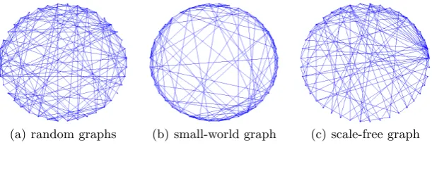
Erd˝os-R´enyi model(ER) [13]: AnERgraphG(n, p) is constructed by con-necting n vertices randomly with probability p. i.e., each edge is included in the graph with probability p independent from every other edge. These models are also calledrandom networks.
Watts and Strogatz model(WS) [14]: AW SgraphG(n, k, p) is constructed in the following way. First construct a regular ring lattice, a graph withn
vertices and each vertex is connected to k nearest vertices, k/2 on each side. Then for every vertex take every edge and rewire it with probabilityp. These models are also calledsmall-world networks.
Barab´asi-Albert model(BA) [15]: ABA graphG(n, n0, m) is constructed
by an initial fully connected graph withn0 vertices. New vertices are added
to the graph one at a time. Each new vertex is connected to m previous vertices with a probability that is proportional to the number of links that the existing nodes already have. These models are also calledscale-free networks.
Figure 2 shows an example of each of these models.
[image:8.595.156.462.354.479.2](a) random graphs (b) small-world graph (c) scale-free graph
Fig. 2.Graph models
amplitudes to more links. The WS network, on the other hand, has more regular structure that allows the wave packet to transmit across the network with high amplitudes.
Fig. 3.Number of links infected with time
The above experiment shows that the WCT behaves differently on different graphs. This suggests that the WCT can be used to quantify the structure of a complex network. In our next experiment, we demonstrate the ability of WCT to distinguish networks with different substructures. For this purpose, we generate 100 graphs for each model withn= 50 + (d−1)k with k= 1,2, ...,100, where
n is the number of vertices. We have chosen the other parameters in such a way so that all three types of graphs with the same number of vertices have approximately the same number of edges. ForER models we choosep= 10/n, for W S models we choose p= 0.25 and k = 8, and forBA models we choose
n0 = 5 and k = 4. For each graph we compute the wave commute time and
average it over all the edges. Figure 4(a) shows the average value for the three different types of graphs. Results suggest that the wave commute time is highly robust in distinguishing the graphs with different structures.
Figure 4(b) shows a similar analysis for vertex commute time, which is defined as the expected number of steps for a random walk starting from a vertexu, hits vertexvand then returns tou. The commute time of a vertexuto a vertexvcan be computed from the eigenvalues and eigenvectors of the normalized Laplacian. Let (λ, φ) be the eigenpair of the normalized Laplacian. Then the commute time is defined as:
CT(u, v) =
|V| X
i=2
r
vol
λiduφi(u)−
r
vol λidvφi(v)
!2
, (7)
Commute Time for Gaussian Wave Packet on a Graph 9
[image:10.595.139.478.112.289.2](a) Wave commute time (b) Vertex commute time
Fig. 4.Wave commute time vs commute time
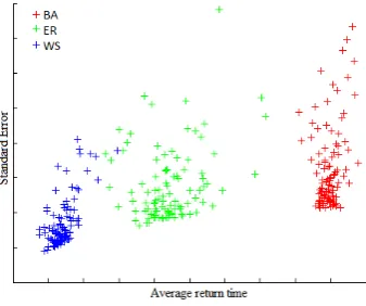
The mean and the standard error of the edge-commute time depend on the regularity structure of the graph. As the regularity of the graph increases, the value of the standard error decreases. Note that the value of WCT depends on the size of the smallest cycle to which the edge belongs. Figure 5 shows the mean values and the standard errors for the graphs generated in the previous experiment. Since WS networks are more regular as compared to BA networks, they therefore have smaller standard errors. Also, if the probabilitypof rewiring is kept low, then the WS network has more small length cycles. Therefore the mean values of WS networks are small as compared to BA networks. Note that ER graphs exhibit more variation in the mean values due to their random struc-ture. Their mean and standard error values lie between that of the BA graphs and the WS graphs.
[image:10.595.224.393.502.643.2]5
Conclusion
In this paper we have studied the properties of the commute time (WCT) and the hitting time (WHT) of a Gaussian wave packet on a graph. The WCT and WHT are based on the solution of the wave equation defined using the edge-based Laplacian of a graph where the initial condition is a Gaussian wave packet on a single edge of the graph. We have shown the application of WCT and WHT for quantifying the structure and information flow of a network. The advantage of using the edge-based Laplacian (EBL) is that this approach is more closely related to mathematical analysis than the usual discrete Laplacian. This allows us to implement equation on graphs which have finite speed of propagation.
References
1. Grenfell, B. T.: Travelling waves and spatial hierarchies in measles epidemics. Na-ture, 716-723 (2001).
2. Abramson, G., Kenkre, V.M., Yates, T.L., Parmenter, R.R.: Traveling Waves of Infection in the Hantavirus Epidemics. Bulletin of Mathematical Biology, 519534 (2003).
3. Passerini, F., Severini, S.: The von neumann entropy of networks. International Journal of Agent Technologies and Systems, 5867 (2009).
4. Han, L., Escolano, F., Hancock, E.R., Wilson, R.C.: Graph characterizations from von Neumann entropy. Pattern Recognition Letters, 1958-1967 (2102).
5. Escolano, F., Hancock, E.R., Lozano, M.A.: Heat diffusion: Thermodynamic depth complexity of networks. Physics Review E, 036206 (2012).
6. Escolano, F., Bonev, B., Hancock, E.R.: Heat Flow-Thermodynamic Depth Com-plexity in Directed Networks. SSPR/SPR, 190-198 (2012).
7. Suau, P., Hancock, E.R., Escolano, F.: Analysis of the Schr¨odinger Operator in the Context of Graph Characterization: SIMBAD 190-203 (2013).
8. Aziz, F., Wilson, R.C., Hancock, E.R.: Gaussian Wave Packet on a Graph. GbRPR, 224-233 (2013).
9. Lee, A. B., Luca, D., Klei, L., Devlin, B., Roeder, K.: Discovering genetic ancestry using spectral graph theory. Genetic Epidemiology, 51-59 (2010).
10. Bradonjic, M., Molloy, M., Yan, G.: Containing Viral Spread on Sparse Ran-dom Graphs: Bounds, Algorithms, and Experiments. Internet Mathematics, 406-433 (2013).
11. Friedman, J., Tillich, J.P.: Wave equations for graphs and the edge based Laplacian. Pacific Journal of Mathematics, 229-266 (2004).
12. Wilson, R.C., Aziz, F., Hancock, E.R.: Eigenfunctions of the edge-based Laplacian on a graph. In Journal of Linear Algebra and its Applications, 4183-4189 (2013). 13. Erd˜os, P., R´enyi A.: On the evolution of random graphs. Publications of the
Math-ematical Institute of the Hungarian Academy of Sciences, 1761 (1960).
14. Watts, D. J., Strogatz, S. H.: Collective dynamics of ’small-world’ networks. Na-ture, 440442 (1998).