Accelerating Markov chain Monte Carlo
via parallel predictive prefetching
The Harvard community has made this
article openly available. Please share how
this access benefits you. Your story matters
Citation Angelino, Elaine Lee. 2014. Accelerating Markov chain Monte Carlo via parallel predictive prefetching. Doctoral dissertation, Harvard University.
Citable link http://nrs.harvard.edu/urn-3:HUL.InstRepos:13070022
Terms of Use This article was downloaded from Harvard University’s DASH repository, and is made available under the terms and conditions applicable to Other Posted Material, as set forth at http://
Accelerating Markov chain Monte Carlo via parallel predictive prefetching
A dissertation presented
by
Elaine Lee Angelino
to
The School of Engineering and Applied Sciences
in partial fulfillment of the requirements
for the degree of
Doctor of Philosophy
in the subject of
Computer Science
Harvard University
Cambridge, Massachusetts
c
Dissertation Advisors Author
Professor Margo Seltzer and Professor Ryan P. Adams Elaine Lee Angelino
Accelerating Markov chain Monte Carlo via parallel predictive prefetching
Abstract
We present a general framework for accelerating a large class of widely used Markov
chain Monte Carlo (MCMC) algorithms. This dissertation demonstrates that MCMC
inference can be accelerated in a model of parallel computation that uses speculation to
predict and complete computational work ahead of when it is known to be useful. By
exploiting fast, iterative approximations to the target density, we can speculatively
evaluate many potential future steps of the chain in parallel. In Bayesian inference
problems, this approach can accelerate sampling from the target distribution, without
compromising exactness, by exploiting subsets of data. It takes advantage of whatever
parallel resources are available, but produces results exactly equivalent to standard serial
execution. In the initial burn-in phase of chain evaluation, it achieves speedup over serial
Contents
1 Motivation and summary 1
2 Markov chain Monte Carlo 7
2.1 Markov chains . . . 8
2.2 Monte Carlo methods . . . 10
2.2.1 Rejection sampling . . . 12
2.2.2 Importance sampling . . . 12
2.2.3 Limitations of Monte Carlo sampling . . . 13
2.3 Markov chain Monte Carlo . . . 14
2.4 Metropolis-Hastings (MH) . . . 15
2.4.1 Factors affecting the behavior of MH . . . 16
2.5 MCMC methods for faster convergence . . . 19
2.5.1 Auxiliary variable methods . . . 19
2.5.2 Ensemble methods . . . 21
2.5.3 Non-reversible methods . . . 22
2.6 Parallel MCMC . . . 23
2.6.1 Parallel ensemble samplers . . . 24
2.6.2 Prefetching . . . 24
2.7 Approximations and large-scale Bayesian inference . . . 26
2.7.1 Embarrassingly parallel, approximate MCMC . . . 27
2.7.2 MCMC with mini-batches . . . 28
3 Predictive prefetching with transition operator approximation 30 3.1 Mathematical framework . . . 31
3.2 Metropolis–Hastings simulation . . . 34
3.2.1 Bit string notation . . . 34
3.2.2 Mapping states to bit strings . . . 35
3.2.3 Computation with respect to a simulation path . . . 36
3.2.4 Using pseudo-randomness . . . 37
3.2.5 Representing computation with the jobtree . . . 38
3.2.6 Metropolis–Hastings with prefetching . . . 40
3.3 Predictive prefetching: Exploiting predictions . . . 42
3.4 An estimator for large-scale Bayesian inference . . . 45
3.5 Speedup with instantaneous, imperfect predictions . . . 48
3.5.2 Worker allocation and expected speedup . . . 50
3.5.3 Speculation plus parallelism at each node . . . 52
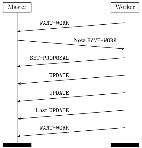
4 System architecture and implementation 54 4.1 Architectural overview . . . 55
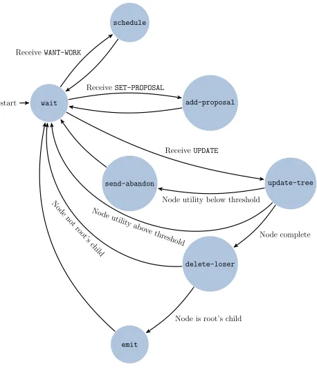
4.1.1 Master state machine . . . 55
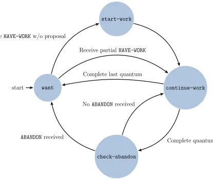
4.1.2 Worker state machine . . . 57
4.1.3 Practical considerations . . . 59
4.2 The jobtree . . . 60
4.3 Selecting high-utility pending nodes . . . 61
4.4 Execution and messaging protocol . . . 62
4.5 Managing pseudo-randomness . . . 67
4.6 Generating proposals . . . 69
4.7 Predictor implementation . . . 70
4.8 Implementation details and plug-in interface . . . 71
5 Empirical evaluation 74 5.1 Example Bayesian inference problems . . . 75
5.1.1 Mixture of multidimensional Gaussians . . . 75
5.1.2 Bayesian Lasso for photovoltaic activity . . . 76
5.2 Adaptive proposal distribution . . . 78
5.3 Assessing chain convergence and quality . . . 80
5.4 Speedup results . . . 82
5.5 Adaptive Metropolis–Hastings behavior . . . 87
5.6 Estimate, error model and predictor behavior . . . 89
5.7 System measurements . . . 97
5.8 System overheads . . . 101
6 Conclusions and generalizations 104
Acknowledgements
This dissertation describes joint work with Eddie Kohler, Amos Waterland, Margo Seltzer,
and Ryan P. Adams. I would like to thank Michael P. Brenner, Ekin Dogus Cubuk, Jonathan
H. Huggins, Varun Kanade, Zhenming Liu, Dougal Maclaurin, and Robert Nishihara for
helpful discussions, Alan Aspuru-Guzik, Johannes Hachmann and Roberto Olivares-Amaya
for the use of the Clean Energy Project dataset and introduction to the cheminformatic
feature set, and Michael Tingley for the derived features used here. Michael I. Jordan
influ-enced writing that appears in Chapter 1. Kevin Swersky, David Duvenaud, Xinghao Pan and
Joseph Gonzalez provided helpful comments on Chapter 6. Andrew C. Miller and Matthew
J. Johnson provided many helpful comments on drafts of this manuscript. This work was
partially funded by DARPA Young Faculty Award N66001-12-1-4219, the National
Insti-tutes of Health under Award Number 1R01LM010213-01, a Microsoft Research New Faculty
Fellowship award, and Google.
I am deeply indebted to Margo Seltzer for supporting my various interests while steering
me toward concrete and fulfilling directions. I would like to thank Ryan P. Adams for sharing
his enthusiasm and ideas on diverse topics, and Eddie Kohler for incredible generosity with
his time and systems expertise. I also thank Michael P. Brenner for putting up with me
all these years. The Harvard School of Engineering and Applied Sciences has given me fine
institutional support. I woud like to acknowledge Women in Machine Learning for having a
profound impact on my research direction. Finally, I am very grateful to many individuals
Margo Seltzer Ryan P. Adams Eddie Kohler Michael P. Brenner
Alecia McGregor Christina Cheuk
Roy Kishony Andrew Murray Pardis Sabeti Frank Solomon
Allison Craney
Adriana Gallegos
Dhruva Kothari Aaron Tjoa
Rianna Stefanakis
Bobby Thompson Ryan LaPerle Jaclyn Parks
Danny Goodman Marsha Berger Jonathan Goodman
Aviva Presser Aiden Erez Lieberman Aiden
Denny Kinlaw Ben Belknap
Daniel Yamins Janice Yamins David Yamins
Justin T. Riley Eric Jones Doug Fritz
Jason Rosenfeld
Uri Braun David Holland Daniel Margo Peter Macko Nicholas Murphy
Kiran-Kumar Muniswamy-Reddy Robin Smogor Susan Welby
Marc Chiarini Lisa Lowy
Ann Marie King Marie Dooley Lisa Frazier Meg Hastings Julie Holbrook
Peter Bailis Karthik Dantu Brian Kate Jason Waterman Jim Waldo
Philip Guo Nils Napp Kirstin Petersen
Heather Pon-Barry Alice Gao Sophia Shao Stacy Wong Elif Yamangil
Neena Kamath Amy Tai Joy Zhang Raina Masand
Jeremy Rassen Pete Wahl Sebastian Schneeweiss
Michael Mitzenmacher Naveen Sinha Brent Heeringa Michael Goodrich
Jonathan Appavoo Efthimios Kaxiras
Steve Chong Greg Morrisett Radhika Nagpal Barbara Grosz
Jeremy Gunawardena
Christos Papadimitriou
Leslie Valiant
Elena Agapie Anna Huang Varun Kanade Justin Thaler
Amos Waterland Dogus Cubuk Miguel Aljacen Miriam Huntley Ben Good
James Zou Zhenming Liu Jon Ullman Thomas Steinke Mark Bun
Kenneth Arnold Pao Siangliulue Bo Waggoner Sam Wiseman
Margo Levine Marie Dahleh Beth Chen Sarah Kostinski
Michael S. Kester Jemila C. Kester Sarah M. Kester Hannah J. Kester
Gregory Valiant Sham Kakade
Teagan Seltzer Tynan Seltzer Keith Bostic
Mary Baker
Eyal Dechter Finale Doshi-Velez David Duvenaud Yakir Reshef
Diana Cai Michael Gelbart Scott Linderman Dougal Maclaurin Robert Nishihara
Oren Rippel Jasper Snoek Kevin Swersky Brian Zhang
Matt Johnson Jonathan Huggins
Andy Miller
Chapter 1
Motivation and summary
A central tool of modern data analysis isinference, the process of estimating structure in data
via probabilistic modeling. The goal is to recover the parameters of a probabilistic description
of data, given a set of observations. In particular, Bayesian inference uses Bayes’ rule to
update a probabilistic description of model parameters as more data are observed. Sadly,
inference is computationally expensive when the underlying functions are high-dimensional
and/or full of many local optima, as is typical with large datasets. In general, there are no
analytic solutions to these problems; there are approximate and simulated approaches, but
these are often slow and do not naturally leverage modern computing resources, such as
clouds.
Inference is dominated by two approaches: usingoptimization procedures to find the best
model parameter setting and the Bayesian approach of integrating with respect to the
rela-tive probabilities of various parameter settings. This thesis focuses on Bayesian procedures,
which have been mostly absent in discussions of large-scale inference until very recently.
While there have been recent successes in scaling inference procedures, most have focused
on optimization.
posterior is proportional to the product of two other probability densities, alikelihood π(x|θ) describing the probability of the data, given the model, and aprior π0(θ) over the model
pa-rameters. Bayesian inference is appealing because the posterior density encodes uncertainty
over model parameters; this uncertainty can then be propagated to downstream applications.
However, there are often no analytic solutions to useful functions of the posterior, such as
expectations; typically these involve integrating over the parameters. While samples from
the posterior can be used to estimate quantities of interest, there is usually no analytic way
to obtain them. This motivates approximate sampling-based methods such as Markov chain
Monte Carlo (MCMC) andimportance sampling. Unfortunately, these methods are difficult
to scale, which has inhibited their application to large datasets.
This thesis focuses on MCMC, a widely used, powerful and general technique for both
optimization and Bayesian inference. In the optimization setting, it stochastically searches
a parameter space for the best setting of θ. In Bayesian inference, it produces a sequence of
samples drawn from a sequence of distributions that converge to the posterior distribution.
These algorithms are typically slow to converge so they must be run for many iterations
before they yield useful output. Furthermore, they are inherentlyserial and thus, in general,
do not parallelize well.
Reliance on serial algorithms is a great frustration given the power of today’s scientific
computing environments, which are highly parallel. Researchers have routine access to
hun-dreds to thousands of parallel cores in multicore environments, where computational work
can be distributed over multiple cores that are able to communicate with one another. Thus,
our ability to perform large-scale Bayesian inference is limited by our algorithms, not our
computational resources.
The pseudocode in Algorithm 1 illustrates the serial nature of many Bayesian inference
procedures: start with some initial setting of model parametersθ0, then iteratively select the
next parameter setting θ1 from some set of choices that depend onθ0, then θ2 from choices
Algorithm 1 Serial Bayesian inference
Specify a dataset x, a posterior density π(θ|x) and an initial parameter settingθ0.
for t in 0, . . . , T do
Generate one or more parameter settings {θ0} that depend onθt.
Select θt+1 from {θ0}by comparing the evaluations of {π(θ0|x)} toπ(θ|x).
end for
Output some function of θ1, θ2, θ3, . . ..
for t > 0 depends on the computationally expensive evaluation of π(θt|x). If we had N cores and could performN iterations at a time in parallel, then we could speed-up execution
by a factor of N. However, since each iteration depends on the last, it is not possible to
skip ahead to later iterations without first completing earlier ones. Specifically, the iteration
indexed by t produces θt+1 in a way that depends on knowing θt, which in turn depends
onθt−1, θt−2, . . . , θ0, only the last of which is known initially.
That said, there is nothing to stop us from materializing predictions for θt and executing
the corresponding iterations on parallel cores. This is a form of speculative execution, the
technique of optimistically performing computational work that might be eventually useful.
This dissertation demonstrates that MCMC inference can be accelerated in a model of parallel computation that uses speculation to predict and complete computational work ahead of when it is known to be useful.
Below, we outline how the remaining chapters demonstrate the veracity of this thesis
statement. In Chapter 2, we review Markov chain Monte Carlo, an algorithmic approach for
stochastically estimating the expectation of a function with respect to a probability
distribu-tion. Computing such an expectation might be an intractable task,e.g., its exact calculation
might involve a sum of exponentially many values or an integral with no known analytic
solution. MCMC combines two powerful ideas – Markov chains and Monte Carlo integration
– and we begin by explaining the basic theory and properties of all three. In particular,
the serial nature and convergence behavior of MCMC algorithms derive from their
under-lying use of Markov chains. The Metropolis–Hastings (MH) algorithm provides a concrete
and limitations of MCMC. The rest of the chapter categorizes existing MCMC algorithms
according to their strategies for improving on na¨ıve algorithms such as MH. The algorithms
in the first of two broad categories attempt to decrease the time to reach convergence; those
in the second make use of parallel resources. We do not provide a complete review of all
MCMC algorithms, which have been reviewed elsewhere, but we do thoroughly summarize
existing parallel MCMC algorithms that use speculative techniques, called prefetching in
this literature. Finally because this thesis is motivated by large-scale Bayesian inference, the
chapter ends with a summary of MCMC algorithms recently proposed for this setting.
The core intellectual contributions of this thesis are in Chapter 3, where we propose
and analyze a new class of prefetching MCMC algorithms. First, we provide a
mathemati-cal language for describing a large class of MCMC algorithms that can be mapped to, and
would benefit from, prefetching. This treatment is more formal and general than what has
been provided by prior prefetching literature but is designed to motivate prefetching and
elucidate its feasibility and validity. For concreteness, the remainder of the thesis focuses
on Metropolis–Hastings, where prefetching requires speculating about the outcome of a
bi-nary condition at each iteration of the algorithm. This motivates predictive prefetching, a
principled framework for exploiting predictions about these binary outcomes so as to most
effectively allocate parallel resources. The goal is to maximize the expected speed-up relative
to serial execution, given parallel cores and predictive information. We derive predictors for
the setting of large-scale Bayesian inference that we later use directly in the empirical
stud-ies of Chapter 5. Finally, since perfect predictions are not normally available, we analyze
the performance of predictive prefetching in terms of expected speed-up as a function of
predictor accuracy and the number of parallel cores.
Chapter 4 describes the design and implementation of a practical parallel system for
predictive prefetching. The system architecture follows a master-worker pattern in which a
single master core maintains information about computational work that might be useful,
of these computations. The master maintains data structures that organize the results of
potentially useful increments of computational work, plus related information. These
incre-ments of work include all those that exactly correspond to equivalent serial execution and are
eventually identified as such with absolute certainty. Workers request work from the master
whenever they are available, the master replies to each worker with a specification of the
work to do, and workers send computed results back to the master. The system guarantees
results equal to serial execution, i.e., invariant to the number of cores used. Since MCMC
algorithms are stochastic, this guarantee depends critically on correct management of the
source of (pseudo)randomness. This issue is subtle and the solution presented here is more
careful than any provided in prior literature on prefetching. The implementation includes a
simple plug-in interface for specifying a concrete instantiation of a MH algorithm via
user-defined functions. We also provide remaining details about specific implementation choices
and artifacts.
Next, in Chapter 5, we present an empirical evaluation of the parallel implementation of
predictive prefetching in a real research computing environment. We select and implement
concrete large-scale Bayesian inference problems involving both synthetic and real datasets.
The efficiency of predictive prefetching depends on the behavior of MH, which in turn
de-pends in a sensitive fashion on parameters that are typically hand-tuned by practitioners
according to heuristic guidelines. Furthermore, this behavior changes – often dramatically –
over the course of running a single instantiation of the algorithm. To execute reasonably
cali-brated experiments, we identify an adaptive MH scheme that eliminates this tuning problem
and requires only a simple extension to our original implementation for MH. We clearly
de-scribe a framework for assessing chain convergence, which we use to identify different regimes
of chain behavior. We present and discuss empirical results for speed-up as a function of the
number of parallel cores used, measured relative to a baseline system implementation with
one master and one worker. The chapter ends with a discussion of the overheads of our
Finally, in Chapter 6 we distill the conclusions of this thesis, including lessons learned and
a map of possible extensions to this work. We will have demonstrated effective use of relatively
na¨ıve prediction strategies, therefore we identify additional promising strategies for predictive
prefetching, emphasizing generic methods based on constructing approximations to a target
density. We also outline technical challenges for predictive prefetching in the context of
more sophisticated MCMC algorithms, then propose and justify potential solutions. We end
with a broad discussion of opportunities for applying speculative execution to algorithms
ranging across various properties: stochastic versus deterministic, exact versus approximate
Chapter 2
Markov chain Monte Carlo
Markov chain Monte Carlo (MCMC) is a widely used, powerful technique for estimating
statistics of an arbitrary distribution Π defined over a state space X. MCMC simulates a
random walk that produces a sequence of samples drawn from a sequence of distributions
that converges to Π. MCMC is typically employed when samples from, or statistics of,
a distribution cannot be obtained analytically, as is often the case with complex,
high-dimensional systems arising across disciplines,e.g., estimating bulk material properties from
molecular dynamics physics simulations or inferring the parameters of Bayesian probabilistic
models describing large datasets.
In this chapter, we first review the two powerful tools underlying MCMC algorithms –
Markov chains and Monte Carlo methods. Next, we introduce MCMC via the well-known
Metropolis-Hastings algorithm, both as a way to concretely exemplify relevant concepts and
to motivate a large body of research whose goal is to design more efficient MCMC algorithms.
We then provide an overview of different classes of these approaches, with greater focus on
the areas that together provide the foundation for a new approach to large-scale MCMC
2.1
Markov chains
Let X be a discrete or continuous state space and let x, x0 ∈ X denote states. A Markov
chain is a discrete-time stochastic process governed by a transition operator T(x→x0) that
specifies the probability of transitioning from a current state x to some next state x0. It is
memoryless in the sense that its future behavior depends only on the current state and is
independent of its past history – this is known as the Markov property.
Many systems can be modeled by Markov chains. For example, an unbiased random walk
on a one-dimensional lattice is described by a Markov chain. The integers modulo k can be
used to index a finite lattice of k states, in which caseX =Zk. The transition operator,
T(x→x−1 mod k) = T(x→x+ 1 modk) =T(x→x modk) = 1
3, (2.1)
describes a random walk on the lattice, with periodic boundaries, that at each time step
either moves to the ‘left’ or ‘right’ by one unit, or stays put, where the three scenarios are
equiprobable. Here, the stationary distribution is simply the uniform distribution over Zk. Given an initial distribution P0(x) overX, a Markov chain evolves this distribution from
one time point to the next through iterative application of the transition operator; after t
steps let us call this distribution Pt(x). Direct simulation of a Markov chain follows this
iterative construction and leads to inherently serial implementations. We are interested in
Markov chains that converge to a unique stationary distribution π(x) in the sense that
lim t→∞P
t(x)→π(x),
for any initial distributionP0(x).
The speed of convergence or mixing time of a Markov chain measures how quickly Pt(x)
approaches π(x); it is typically defined with respect to a distance measure between
expected number of steps t such that DKL(π(x) k Pt(x))< , for some appropriate >0,
where DKL(PkQ) is the Kullback-Leibler divergence of two distributions P and Q, and we
think of Q as an approximation to P (Kullback and Leibler, 1951). Convergence behavior
depends on the properties of the state space X – e.g., whether it is discrete or continuous,
its dimensionality – and the behavior of the transition operator.
For example, consider a simulation of a one-dimensional,k-state random walk, described
by the transition operator in Eq. 2.1. The mixing time is O(k2), i.e., the simulation
re-quires O(k2) steps to ‘forget’ the initial condition and look reasonably like the uniform
stationary distribution. In contrast, consider a deterministic transition operator that always
moves to the ‘right’, i.e.,T(x→x+ 1) = 1. This time, simulation requires only O(k) steps
to approach the uniform stationary distribution. While this simple example represents an
extreme case that is not useful for typical applications, it illustrates how two Markov chains
can have the same stationary distribution but different convergence behavior. A major area
of Markov chain research is understanding how to design efficient transition operators that
converge quickly, as doing so has direct practical consequences for their simulation.
For a transition operator T(x → x0) to have π(x) as its stationary distribution, its
application must leave π(x) invariant over the entire space, i.e.,
X
x∈X
T(x→x0)π(x) = π(x0), ∀x0 ∈ X
for a discrete state space, or
Z
X
T(x→x0)π(x)dx=π(x0), ∀x0 ∈ X (2.2)
for a continuous state space; this thesis will focus on continuous state spaces. For the
sta-tionary distribution to be unique, i.e., not depend on the initial distribution, the Markov
chain must be irreducible: for any x, x0 ∈ X such that π(x), π(x0) > 0, it must be possible
involves designing a transition operator that has as its stationary distribution some target
distribution of interest – this is the main idea behind Markov chain Monte Carlo methods.
In restricted cases it is easy to show that a transition operator has a certain stationary
distribution. Notably, when a transition operatorT(x→x0) isreversible, it satisfies detailed
balance with respect to a distribution π(x),
T(x→x0)π(x) =T(x0 →x)π(x0), (2.3)
and it is easy to show that π(x) is its stationary distribution. Integrating over X on both
sides gives:
Z
X
T(x→x0)π(x)dx =
Z
X
T(x0 →x)π(x0)dx
= π(x0)
Z
X
T(x0 →x)dx
= π(x0),
which is precisely the required condition from Eq. 2.2. We can interpret Eq. 2.3 as stating
that, for a reversible Markov chain starting from its stationary distribution, any transition
x→x0 is equilibrated by the corresponding reverse transition x0 →x. As we will see, many
MCMC methods are based on deriving reversible transition operators. A transition operator
that is not reversible is callednon-reversible; it is generally more difficult to manipulate and
prove statements about these.
For a formal introduction to Markov chains, see the book by Meyn and Tweedie (1993).
2.2
Monte Carlo methods
Monte Carlo methods are a broad class of algorithms that simulate many repeated
ran-dom samples to estimate some quantity of interest. For example, the following procedure
f : [a, b]→R+, where −∞< a < b <∞:
1. Draw a box around f with vertical boundaries set by the interval [a, b] and horizontal
boundaries set by 0 and an upper boundm on the maximum value off in the interval.
2. Sample a large number of random points (x, y) uniformly within the box and for each,
determine whether the point falls below or above f by computing whether f(x)< y.
3. Let r be the fraction of points such that f(x) < y. Since the total area of the box is
m(b−a), multiplying byr provides an estimate forRb
a f(x)dx.
More generally, when we can think of an integral as an expectation, Monte Carlo
inte-gration invokes the law of large numbers to estimate this expectation via a sample average.
Specifically, if we can write an integral as the expectation of a functionf(x) with respect to
a distribution Π with probability density functionπ(x),
EΠ(f) =
Z
f(x)π(x)dx, (2.4)
then we can estimate this integral by averaging over a set of samples {xn}Nn=1 from Π as:
¯
fN ≡ 1
N
N
X
n=1
f(xn).
Since the samples are independent, as long as the expectation in Eq. 2.4 exists and is finite,
this sum obeys the law of large numbers. Hence, the estimate is unbiased and its variance
scales as the inverse sample size 1/N, or equivalently, its error scales as 1/√N. In our example
above, the integral of f(x) on the interval [a, b] can be thought of as an expectation with
respect to the uniform distribution on [a, b].
Monte Carlo integration thus requires sampling from a distribution, which is sometimes
straightforward, as with the uniform and normal distributions, but in general requires
this issue in restricted settings: rejection sampling and importance sampling. Their
limita-tions and inefficiencies will help motivate Markov chain Monte Carlo methods, which are
more sophisticated but related techniques. For simplicity, we describe these procedures with
respect to one-dimensional normalized probability densities; both can be generalized.
2.2.1
Rejection sampling
Rejection sampling uses one distribution to sample from another by exploiting information
relating the two; von Neumann (1951) provided an algorithm for this method. Suppose
that we want to sample from a target distribution Π with probability density functionπ(x).
Suppose further that we can sample from aproposal distribution Qwhose probability density
functionq(x) can be scaled by a constant factorγto provide an upper bound onπ(x),e.g., we
might be able to scale a normal distribution so that our distribution of interest lies below it
everywhere. If we satisfy these requirements, then we can use rejection sampling to generate
proposals fromQ that we stochastically accept or reject according to the relative difference
between γq(x) and π(x). Specifically, to produce one sample:
1. Generate a proposal xby drawing a sample from the proposal distribution Q.
2. Draw a sample y uniformly from the interval [0, γq(x)].
3. If y < π(x), accept x. Otherwise, reject x and return to Step 1.
Rejection sampling is most efficient in the limit where the scaled proposal density equals the
target density, in which case all proposals are accepted. More generally, in expectation, this
procedure accepts proposals at a rate given by R π(x)/(γq(x))dx≤1.
2.2.2
Importance sampling
Similar to rejection sampling, importance sampling also uses information from one
and Q as above, where this time we can simply think of q(x) as an approximation to π(x);
i.e., we do not require some γq(x) that is an upper bound to π(x). Suppose we want to
compute the expectation of some function f(x) with respect to the distribution Π:
EΠ(f(x)) =
Z
f(x)π(x)dx.
By multiplying and dividing by q(x) inside the integral,
EΠ(f(x)) =
Z
f(x)π(x)
q(x) q(x)dx≡EQ(f(x)w(x)),
we change nothing, but can interpret this new expression as the expectation off(x) weighted
by w(x) = p(x)/q(x) with respect to Q. We can Monte Carlo estimate this integral using a
set of samples {xn}Nn=1 fromQ:
1
N
N
X
n=1
f(xn)w(xn).
The quality of this estimator depends on how much f(x)w(x) varies – ideally this
quan-tity would be constant with respect to x. Some historical notes and a list of references on
importance sampling can be found in the textbook by Gelman et al. (2003).
2.2.3
Limitations of Monte Carlo sampling
The primary limitation of both rejection sampling and importance sampling is that for
these methods to be feasible and practical, each requires a proposal distribution that can
be sampled easily and is in some sense close to the target distribution. To produce samples,
both methods use a set of independent samples from the proposal distribution; rejection
sampling selects from among the proposals and importance sampling ‘fixes up’ the proposals
2.3
Markov chain Monte Carlo
Markov chain Monte Carlo (MCMC) methods simulate a Markov chain whose stationary
distribution is equal to a target distribution of interest. When this Markov chain is simulated,
it produces samples from a sequence of distributions that asymptotically equals the target
distribution. The principles of Monte Carlo integration, estimation and sampling thus apply
to these samples in the asymptotic limit. Concretely, for a Markov chain started from its
stationary distribution Π with density π(x), a sequence of N samples {xn}Nn=1 can be used
to estimate an expectation EΠ(f) =
R
Xf(x)π(x)dx using Monte Carlo integration via the sample average ¯fN = N1
PN
n=1f(xn). The efficiency of a MCMC transition operator can be
analyzed with respect to both the variance of this estimator, also known as the asymptotic
variance, as well as the speed of convergence or mixing time. In practice, we use samples
produced by simulated chains of finite length, typically started away from stationarity. The
materialized sequence of samples obeys the Markov property and is correlated, which is
in contrast to the independent samples obtained by simple Monte Carlo methods such as
rejection sampling and importance sampling.
The remaining sections of this chapter give an incomplete overview of MCMC
algo-rithms for sampling applications, with greater emphasis on certain procedures either for the
purpose of providing general background or to review those most directly related to this
thesis. First, we describe the Metropolis-Hastings (MH) algorithm, a canonical and simple
MCMC method. We use MH to build some intuition for the behavior of MCMC algorithms,
and to illustrate its limitations that motivate more sophisticated approaches. The following
two sections classify these further approaches into serial algorithms designed to converge
more quickly than MH and parallel algorithms. Finally, we briefly review MCMC algorithms
that exploit common features of Bayesian inference problems. For a general introduction to
2.4
Metropolis-Hastings (MH)
The Metropolis-Hastings (MH) algorithm simulates a Markov chain, over a state space X,
with stationary distribution equal to some target distribution of interest. Given an initial
statex0, a target distributionπ and a proposal functionq(x0|x), MH generates a sequence of
states x1, . . . , xT ∈ X drawn from a sequence of distributions that converges to the target.1
We provide pseudocode for MH in Algorithm 2. Each iteration, a proposal for the next
state x0 is drawn from the proposal distribution, conditioned on the current state x; e.g., a
common choice is to sample from a Gaussian centered at x. The proposal is stochastically
accepted with probability given by theacceptance ratio,
r= π(x
0)q(x|x0)
π(x)q(x0|x), (2.5)
via comparison to a random variateudrawn uniformly from the interval [0,1]. Ifu < r, then
the next state is set to the proposal, otherwise, the proposal is rejected and the next state is
set to the current state. MH is a generalization of theMetropolis algorithm (Metropolis et al.,
1953), which requires the proposal distribution to be symmetric, i.e., q(x0|x) = q(x|x0), in
which case the acceptance ratio is simplyr =π(x0)/π(x). Hastings (1970) later relaxed this
by showing that the proposal distribution could be arbitrary.
The MH algorithm can be viewed as a biased random walk that always accepts proposals
whenπ(x0)q(x|x0)> π(x)q(x0|x) and stochastically rejects them otherwise; for a symmetric
proposal distribution, these scenarios can be interpreted as accepting ‘uphill’ proposals and
stochastically rejecting ‘downhill’ proposals. We can see that the stationary distribution is
indeed π by showing that the MH transition operator satisfies detailed balance, as defined
1As is common in the literature, we will henceforth use the same symbol to refer to both a distribution
Algorithm 2 Metropolis-Hastings
Input:Initial state x0, number of iterations T, targetπ(x), proposalq(x0|x)
Output:Samples x1, . . . , xT
for t in 0, . . . , T −1 do
x0 ∼q(x0|xt) . Generate proposal
r← π(x
0)q(x
t|x0)
π(xt)q(x0|xt)
. Compute acceptance ratio
u∼Unif(0,1) . Draw random number
if u < r then
xt+1 ←x0 . Accept proposal
else
xt+1 ←xt . Reject proposal
end if end for
in Eq. 2.3. From the algorithm description, the MH transition operator is:
T(x→x0) = min(1, r)q(x0|x) = min
1,π(x
0)q(x|x0) π(x)q(x0|x)
q(x0|x).
We can verify the detailed balance condition as follows:
T(x→x0)π(x) = min
1,π(x
0)q(x|x0) π(x)q(x0|x)
q(x0|x)π(x)
= min (π(x)q(x0|x), π(x0)q(x|x0))
= min
π(x)q(x0|x)
π(x0)q(x|x0),1
q(x|x0)π(x0)
= T(x0 →x)π(x0).
2.4.1
Factors affecting the behavior of MH
The MH algorithm is both simple to implement and quite general; it is thus appealing and
widely applicable. However, the MH algorithm has a major drawback – it can be slow to
converge. This is due to the fact that the steps of the underlying Markov chain are correlated,
which can be viewed as random walk or diffusive behavior. One broad strategy for increasing
diffusion; we survey several techniques for doing so in the next section.
Within the MH framework and given a target density, the variable parameters are the
proposal distribution and the initial condition. Let us first consider the proposal distribution.
For example, for a one-dimensional continuous target density, if we restrict the proposal
distribution to be Gaussian and centered at the current state, q(x0|x) =N(x0|x, σ2), then
there is a single tuning parameter: the distribution’s standard deviation σ, which gives the
expected ‘step size’ of the proposal with respect to the current state. This affects the MH
acceptance rate, which we also refer to as the acceptance probability, i.e., the fraction of
proposals that are accepted.
To illustrate the relationship between the proposal distribution and the acceptance rate,
consider unimodal target and proposal distributions. Suppose that we are able to initialize
MH at a state close to the target distribution’s mode with respect to its width. Intuitively,
if the proposal step size is large compared to the width of the target, then proposals will
tend to fall in faraway, low-probability regions, resulting in a low acceptance rate. On the
other hand, if the step size is very small, then the target density at the proposal will be very
close to that at the current state, in which case the algorithm will tend to accept proposals,
but the samples will be highly correlated and the chain will take a long time explore the
area under the target density. This suggests that there is some notion of an optimal MH
acceptance rate corresponding to some intermediate proposal step size.
A classic result is that the optimal value for the MH acceptance rate is 0.234, derived
for the scenario where the target and proposal distributions are multidimensional Gaussians,
in the limits where the chain has converged and the number of dimensions tends to
infin-ity (Roberts et al., 1997). A heuristic widely followed by practitioners is to tune the proposal
distribution to obtain an observed acceptance rate of about 0.234.
The sensitivity of the acceptance rate as a function of the proposal distribution also
explains why the MH algorithm has trouble sampling from multimodal target densities.
separated by low-probability regions that are difficult for a simulated MH chain to traverse.
In these cases, the MH algorithm tends to get ‘stuck’ for many iterations around local modes,
instead of sampling globally from the entire distribution. In practice, a MH simulation tends
to find the mode closest to the initial state and then samples the area around this mode.
Given target and proposal distributions, the only other specification required by the MH
algorithm is an initial state. Clearly, it is desirable for the initial state to be close to some
probable region of the target density – a ‘bad’ initial state combined with the random walk
nature of chain simulation yields initial samples that are not representative of the target.
This initial portion of a MCMC simulation, before convergence, is sometimes calledburn-in.
The behavior of a MCMC simulation during burn-in is different from that after
conver-gence, because the shape of the target density differs far from versus close to the bulk of
its mass. Specifically, the target density tends to be ‘flatter’ or ‘less steep’ around a mode
compared to less probable regions. This characterization interacts with proposal generation,
resulting in acceptance behavior that changes from burn-in to convergence.
To illustrate differences in MCMC behavior between burn-in and convergence, consider
MH for a Gaussian target distribution. Typically, a MCMC simulation is initiated at some
informed guess that is still somewhat far from higher probability regions of the target;
assuming it is well-behaved, the chain should eventually spend more time in these regions.
A Gaussian distribution has its mass concentrated around a single mode. A region close to
this mode can be well-approximated by an upside down parabola – a quadratic function –
while the tails fall off exponentially quickly. Suppose also that our proposal distribution is
symmetric and its width is not large compared to the width of the target. In the region
close to the target mode, the target densities evaluated at two nearby states will tend to
be comparable values. In the context of MH, the acceptance ratio r will be well within
the interval [0,1] and the decision to accept or reject a proposal depends on bothr and the
random variateu. If we consider two nearby states in the tail regions, then the target density
will be close to either 0 or 1, so the random variate u has little influence over whether a
proposal is accepted. As we will see later, these differences between chains during burn-in
and convergence have implications for the performance of our new approach to MCMC as
well as our empirical studies.
2.5
MCMC methods for faster convergence
In this section, we survey classes of MCMC algorithms designed to converge more quickly
than the MH algorithm by reducing the correlation between successive states. We do not
provide a thorough review, as the methods we develop in this thesis do not build directly
on these techniques. However, we do describe specific algorithms both for concreteness,
and because we will later consider them within the context of predictive prefetching, a new
framework we present in Chapter 3.
2.5.1
Auxiliary variable methods
Given a target density π(x), we can introduce an auxiliary variable y and define a new
density π(x, y) such that R
π(x, y)dy =π(x), i.e., marginalizing out y the yields the target.
Auxiliary variable methods design MCMC sampling schemes over the space of a new joint
distribution; after sampling from π(x, y), one obtains samples fromπ(x) simply by ignoring
the y values. While it would seem less desirable to sample from a higher dimensional space,
it is possible to design transition operators over the joint space that marginally sample from
the target in a way that is more efficient than Metropolis-Hastings.
For example, consider a one-dimensional target density π(x) : R → R+. Sampling
from π(x) yields a sequence of samples along the real line. Now consider a representation
of the target in the (x, y)-plane such that y = π(x). If we sample a set of points {(xi, yi)}
uniformly within the two-dimensional area between π(x) and the x-axis, then marginally,
sampling and Hamiltonian Monte Carlo.
Slice sampling methods are based on the above idea, sampling from the joint
distri-bution π(x, y) by iteratively sampling each variable marginally (Neal, 2003). Given some
state xi, the procedure constructs yi and then the next xi+1 as follows:
1. Sample yi ∼π(yi|xi) by sampling uniformly from the (vertical) interval [0, π(xi)].
2. Sample xi+1 ∼π(xi+1|yi) by sampling uniformly from the (horizontal) intervals where
π(x)> yi.
We think of yi as defining a horizontal ‘slice’ through the distribution. Slice sampling has
multiple advantages over Metropolis-Hastings. The procedure has the opportunity to mix
well with respect to sampling from the target distribution, because a horizontal slice may
correspond to a large domain that is sampled uniformly, so xi+1 can be very far from xi. In
practice, it can be tricky to sample the xi since doing so in full would require constructing
the inverse ofπ(x), but there are various procedures for avoiding this issue while maintaining
correctness. Notice also that there is no proposal distribution in slice sampling, which means
fewer tuning parameters.
Hybrid Monte Carlo (HMC) introduces an auxiliary ‘momentum’ variable to embed the
action of sampling from the target density π(x) within a physical system described by
clas-sical mechanics (Duane et al., 1987); it is also calledHamiltonian Monte Carlo (Neal, 2010).
First, think of (x,−π(x)) as defining an ‘upside down’ surface where the original modes
ofπ(x) are ‘valleys’ and low-probability regions are ‘uphill.’ Now consider a frictionless puck
with massmmoving around this surface – its dynamics will be described by its position and
its momentum. HMC generates a proposal for a Metropolis algorithm by giving the puck a
kick in some direction with some velocity, both random. The puck’s trajectory is simulated
for some fixed amount of time τ by integrating the system’s equations of motion; the final
position at time τ is the proposal. This can generate faraway but useful proposals because
regions and loses momentum by moving uphill toward low-probability regions.
2.5.2
Ensemble methods
Ensemble (or population) methods run multiple chains and accelerate mixing by sharing
in-formation between the chains. Examples include affine-invariant ensemble sampling
(Good-man and Weare, 2010) and generalized elliptical slice sampling (Nishihara et al., 2014).
Below, we focus on a class of ensemble approaches known as annealing methods.
Recall that the MH algorithm has trouble sampling from multimodal distributions.
In-formally, ‘flatter’ distributions are easier to sample from compared to ‘peaky’ distributions,
especially multimodal ones. Now consider the probabilistic interpretation of a physical
multi-state system at temperature τ >0: for a statex∈ X, its probabilityp(x) is proportional to
the exponential of the negative of its energyE(x) divided by the temperature, i.e.,
p(x)∝exp(−E(x)/τ). (2.6)
For a given system defined by states and their energies, raising the temperature has the
effect of flattening the distribution over those states, while maintaining important features.
Annealing methods leverage this intuition to sample more efficiently from difficult targets.
As an example of a popular annealing method, we describeparallel tempering (Iba, 2001).2
Letπ(x) be the target density over a state spaceX. The idea is to construct a single Markov
chain on the product spaceXK corresponding to anensemble ofKMetropolis-Hastings
simu-lations of the system specified byπ(x) and Eq. 2.6 or its continuous analog, each at a different
temperature. Simulations at higher temperatures explore the space more quickly than those
at lower temperatures, and they can share information through interactions. One of the K
simulations is constructed to marginally have as its stationary distribution the target π(x).
Explicitly, we can define the system via an energy function of the form E(x) = −log(π(x)).
Now we specify K distributions:
πk(x)∝exp(−E(x)ck), k= 1, . . . K,
whereck can be interpreted as an inverse temperature. Notice thatck = 1 yieldsπk(x) equal
to the target π(x), and ck = 0 results in a constant. Thus to obtainK copies of the system,
with one equal to the target and the rest at higher temperatures, we can choose the ck so
that c1 = 1> c2 > c3 >· · ·> cK ≥0. In each iteration of the algorithm, the K simulations
are advanced according to a MH acceptance rule, but they are also allowed to interact,e.g., a
pair of simulations may exchange states. Thus, the slower mixing chain indexed byk = 1 may
jump to states explored by faster mixing chains at higher temperatures. Parallel tempering is
popular because its implementation is a straightforward modification to the MH algorithm.
There are several additional classes of annealing methods and other ensemble methods;
an excellent review can be found in the PhD thesis by Murray (2007).
2.5.3
Non-reversible methods
The methods described above are representative of the rich menagerie of MCMC algorithms
developed using reversible Markov chains where the probability that the chain is in state x
and transitions to state x0 is equal to the probability that it is in state x0 and transitions
tox. This condition of detailed balance is straightforward to check, which helps explain the
invention of many reversible MCMC methods. Recall that the goal of these methods is to
discourage the diffusive behavior of simple Metropolis-Hastings. Intuitively, diffusion is not
an efficient mechanism for mixing, say, a cake batter – one uses a spoon or electric mixer to
induce a flow that is not equilibrated by a flow in the opposite direction.
Such non-reversibility that discourages ‘backtracking’ has been difficult to study; a
hand-ful of articles describe methods limited to discrete state spaces. These include the theoretical
au-thors start with a reversible unbiased random walk on a one-dimensional finite lattice and
then make two copies of the state space, one ‘upstairs’ for transitions to the ‘right’ and one
‘downstairs’ for transitions to the ‘left’, plus transitions between the two levels. This
non-reversible chain converges more quickly according to two different distance metrics. Geyer
and Mira (2000) reanalyze the same system, this time with respect to asymptotic variance,
and find that the most efficient version of the non-reversible chain sweeps through the states
in a deterministic way. In a related fashion, Neal (2004) constructs non-reversible chains
from reversible chains and demonstrates that their asymptotic variance is no worse than the
original reversible chains. Other non-reversible schemes are inspired by non-diffusive physical
systems, such as a method for inserting ‘vortices’ by Sun et al. (2010).
2.6
Parallel MCMC
The most obvious way to parallelize MCMC is to run independent simulations in parallel
and aggregate their samples. However, this embarrassingly parallel approach does not help
to reduce the mixing time, which can be prohibitively long and would be replicated across
the parallel instances.
In MCMC, the computational cost is most often determined by the expense of
evaluat-ing the target density relative to the mixevaluat-ing time. For example in Metropolis–Hastevaluat-ings, this
cost is incurred when the target is evaluated to determine the acceptance ratio of a
pro-posed move. We focus on the increasingly common case where the target is expensive and
the dominant computational cost. This evaluation can sometimes be parallelized directly,
e.g., when the target function is a product of many individually expensive terms. This
some-times arises in Bayesian inference if the target can be easily decomposed into one likelihood
term for each data item. Scalability (i.e., practically achievable speedup) in this setting is
limited by the communication and computational costs associated with aggregating the
that accelerate MCMC via other sources of parallelism into two classes: parallel ensemble
sampling and prefetching.
2.6.1
Parallel ensemble samplers
The ensemble methods discussed earlier run multiple chains that can be simulated in parallel,
where any information sharing between chains requires communication. Examples include
parallel tempering, described in Section 2.5.2, the emcee implementation (Foreman-Mackey
et al., 2012) of affine-invariant ensemble sampling (Goodman and Weare, 2010) and a parallel
implementation of generalized elliptical slice sampling (Nishihara et al., 2014).
2.6.2
Prefetching
The second class of parallel MCMC algorithms uses parallelism through speculative
execu-tion to accelerate individual chains. This idea is called prefetching in some of the literature
and appears to have received only limited attention. To the best of our knowledge,
prefetch-ing has only been studied in the context of the MH algorithm where, at each iteration, a
single new proposal is drawn from a proposal distribution and stochastically accepted or
rejected. As shown in Algorithm 2, the body of a MH implementation is a loop containing
a single conditional statement and two associated branches. We can thus view the possible
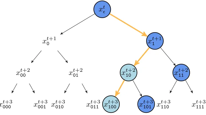
execution paths as a binary tree, illustrated in Figure 2.1. The vanilla version of prefetching
speculatively evaluates all paths in this binary tree (Brockwell, 2006). The correct path will
be exactly one of these, so with J cores, this approach achieves a speedup of log2J with
respect to single core execution, ignoring communication and bookkeeping overheads.
Na¨ıve prefetching can be improved by observing that the two branches are not taken
with equal probability. On average, the reject branch tends to be more probable; the classic
result for the optimal MH acceptance rate is 0.234 (Roberts et al., 1997), so most prefetching
scheduling policies have been built around the expectation of rejection. Let α ≤0.5 be the
x
tx
t0+1x
t00+2x
t000+3x
t001+3x
t01+2x
t010+3x
t011+3x
t1+1x
t10+2x
t100+3x
t101+3x
t11+2x
t110+3x
t111+3Figure 2.1: Metropolis–Hastings conceptualized as a binary tree. Nodes at depthdcorrespond to iteration d, where the root is at depth 0, and branching to the right/left indicates that the proposal is accepted/rejected. Each subscript is a sequence, of length d, of 0’s and 1’s, corresponding to the history of rejected and accepted proposals with respect to the root.
speculatively evaluates only along the ‘reject’ branch of the binary tree; in Figure (2.1), this
corresponds to the left-most branch. In each round of their algorithm, only the first k out
ofJ −1 extra cores perform useful work, wherek is the number of rejected proposals before
the first accepted proposal, relative to the root of the tree. The expected speedup is then:
1 + E(k)<1 +
∞
X
k=0
k(1−α)kα <1 + 1−α
α =
1
α.
The first term on the left is due to the core at the root of the tree, which always performs
useful computation in prefetching schemes. For an acceptance rate of α= 0.23, this scheme
yields a maximum expected speedup of about 4.3, reaching about 4 with 16 cores, and thus
is more limited than the na¨ıve prefetching policy since it essentially cannot take advantage
of additional cores. Byrd et al. (2010) later considered the special case where the evaluation
of the target occurs on two timescales, slow and fast. This method, calledspeculative chains,
modifies speculative moves so that when the target evaluation is slow, available cores are
Further extensions to the na¨ıve prefetching scheme allocate cores according to the
op-timal ‘tree shape’ with respect to various assumptions about the probability of rejecting a
proposal, i.e., by greedily allocating cores to nodes that maximize the depth of speculative
computation expected to be correct (Strid, 2010). Next, we summarize Strid’s schemes and
reference related ideas. Static prefetching assumes a fixed acceptance rate; versions of this
were proposed earlier in the context of simulated annealing (Witte et al., 1991). Dynamic
prefetching estimates the acceptance probabilities,e.g., at each level of the tree by drawing
empirical MH samples (100,000 in the evaluation), or at each branch in the tree by
com-puting min(β,rˆ) where β is a constant (β = 1 in the evaluation) and ˆr is an estimate of the
MH acceptance ratio based on a fast approximation to the target function. Alternatively,
Strid proposes using the approximate target function to identify the single most likely path
on which to perform speculative computation. Strid also combines prefetching with other
sources of parallelism to obtain a multiplicative effect. To the best of our knowledge, these
prefetching methods have been evaluated on up to 64 cores, although usually many fewer.
In the next chapter, we propose predictive prefetching, a new scheme that, like Strid’s
dynamic prefetching, uses an approximation to the target function to predict what
compu-tations to prefetch. There are several fundamental differences between our work and Strid’s.
Most critically, we model the error of the target density approximation, and thus the
un-certainty of whether a proposal will be accepted. In addition, we identify a broad class of
MCMC algorithms that could benefit from prefetching, not just Metropolis–Hastings, and
we show how prefetching can exploit a series of approximations, not just a single one.
2.7
Approximations and large-scale Bayesian inference
Real-world problems are rarely amenable to exact inference, so they require approximate
inference in the form of Monte Carlo estimates orvariational approximations. Unfortunately,
target posterior density may become expensive to evaluate. This challenge has motivated
new methods for inferential computation that can take advantage of approximations to the
target density, most often by examining only a subset of the data, or by exploiting closed
form approximations such as Taylor series (Christen and Fox, 2005), or by fitting linear or
Gaussian process regressions (Conrad et al., 2014).
In Bayesian inference, the target density involves a likelihood, which often decomposes
into a product of many factors corresponding to data items, e.g.,
π(θ|x) =π0(θ)π(x|θ) = π0(θ)
N
Y
n=1
π(xn|θ). (2.7)
Below, we survey MCMC sampling schemes that exploit this factorization property,
moti-vated by large-scale Bayesian inference with large datasets.
2.7.1
Embarrassingly parallel, approximate MCMC
Several authors have suggested partitioning a large dataset into multiple shards and running
MCMC inference on each partition separately across parallel cores. Each ofJshards{x(j)}J j=1
defines what is sometimes called a subposterior:
π(j)(θ|x(j)) =π0(θ)1/J
Y
x∈x(j)
π(x|θ), j = 1, . . . , J.
The contribution from the original prior is down-weighted so that the original posterior is
equal to the product of the J subposteriors, i.e., π(θ|x) = QJ
j=1π
(j)(θ|x(j)). However, it
is not clear how to combine the samples from the J subposteriors in a coherent fashion to
estimate functions of the desired full posterior. Below, we describe three recent efforts.
Neiswanger et al. (2014) explore three potential solutions, ranging from parametric to
non-parametric and semi-parametric models. For example, their parametric model invokes
Gaus-sian in the limit of many data items, they fit each subposterior with a GausGaus-sian, and then
approximate the full posterior as a product of these approximate subposteriors.
Scott et al. (2013) propose consensus Monte Carlo, which combines the subposteriors
through a weighted average. For Gaussian models, the optimal weight of thejth subposterior
is Wj = Σ−j1, the inverse of the covariance matrix Σj of the subposterior. Assuming a
Gaussian model, the authors Monte Carlo estimate Σj using the empirical sample variance
from the corresponding subposterior.
Finally, Wang and Dunson (2013) propose a Weierstrass sampler for parallel MCMC on
independent data partitions; these authors provide analytic bounds on the approximation
error of their sampler, which appears to be more robust than those described above.
2.7.2
MCMC with mini-batches
Other methods for accelerating MCMC sampling in the case of large-scale Bayesian inference
are inspired by stochastic gradient descent. Traditional gradient descent performs
optimiza-tion by iteratively computing and following a local gradient that depends on a sum of terms
corresponding to data items (Dennis and Schnabel, 1983). Stochastic gradient descent is
remarkably simple and effective: at each iteration, it uses an approximate gradient based
on only a random subset of data, called a mini-batch, or even just a single datum
(Mu-rata, 1998). Stochastic variational inference techniques adapt these ideas to variational
in-ference (Hoffman et al., 2013), a class of Bayesian procedures that can be efficient but are
only approximate in the sense of lacking MCMC’s feature of asymptotic correctness.
With MCMC, the idea is to evaluate an approximate posterior whose likelihood term
is a noisy estimate based on sampling only one or a few data items. Recent approaches
have implemented efficient transition operators that lead to approximate stationary
distri-butions (Welling and Teh, 2011; Ahn et al., 2012; Korattikara et al., 2014; Bardenet et al.,
2014; Doucet et al., 2014). Other recent work uses a lower bound on the local likelihood
data at each iteration (Maclaurin and Adams, 2014).
In the rest of this thesis, we focus on accelerating MCMC by combining parallelism with
approximations to the transition operator through prefetching ideas. Notably, we arrive at
Chapter 3
Predictive prefetching with transition
operator approximation
We attack the general problem of accelerating MCMC algorithms by using speculative
exe-cution to parallelize them. In the previous chapter, our survey of MCMC methods included
this approach, sometimes called prefetching. An effective prefetching implementation must
overcome several challenges, such as correctness. For example, for the results of prefetching
to exactly equal those of a serial execution, care is required in the treatment of
pseudo-randomness (i.e., each node’s source of randomness must produce the same results as it
would in a serial execution); slapdash treatment risks introducing biases. But the key
chal-lenge for prefetching is performance. A na¨ıve scheduling scheme always requires≈2J parallel
cores to achieve a speedup of J. As we saw, this speedup can be improved by leveraging
in-formation about the average proposal acceptance rate (Strid, 2010). In particular, if most
proposals are rejected, a prefetching implementation can improve its speedup by
prefetch-ing more heavily along the reject path. Although in practice the optimal acceptance rate is
less than 0.5 (Roberts et al., 1997), extremely small acceptance rates, which lead to good
speedup, are accompanied by less effective mixing. If the acceptance rate is set to something
In this chapter, we propose predictive prefetching, a new scheduling approach that uses
local information to improve speedup relative to other prefetching schemes. First, we
pro-vide a general mathematical framework that allows us to identify a broad class of MCMC
algorithms that can benefit from prefetching. Second, we carefully reason about Metropolis–
Hastings in a way that maps naturally to prefetching schemes. Next, we describe our
predic-tive prefetching scheme, where we adappredic-tively adjust speculation based not only on the local
average proposal acceptance rate – which changes as evaluation progresses – but also on the
actual random deviate used at each state. In particular, we describe how we make use of
any available fast approximations to the transition operator. Though these approximations
are not required, when they are available or learnable, we leverage them to make better
scheduling decisions. For the special case of large-scale Bayesian inference, we develop a
se-ries of increasingly expensive but more accurate approximations. These decisions are further
improved by modeling the error of these approximations, and thus the uncertainty of the
scheduling decisions. Performance depends critically on how we model the approximations,
and a key insight is in our error model for this setting; much smaller error, and therefore
more precise predictions, are obtained by modeling the error of the difference between two
proposal evaluations, rather than evaluating the errors of the proposals separately. Finally,
we provide a theoretical analysis of speedup due to predictive prefetching as a function of
predictor accuracy and the number parallel cores. In the next chapter, we describe the
de-tails of our system design and implementation, and in the following chapter, we present our
actual empirical results.
3.1
Mathematical framework
Consider a transition operatorT(x→x0) which hasπ as its stationary distribution on state
space X. Simulation of such an operator typically proceeds using an ‘external’ source of
uni-formly on the unit hypercube, denoted asU. The transition operator is then a deterministic
function from the product space ofU andX back toX,i.e., T :X × U → X. Most practical
transition operators – Metropolis–Hastings, slice sampling,etc.– are actually compositions of
two such functions, however. The first function produces a countable set of candidate points
in X, here denoted Q:X × UQ→ P(X), where P(X) is the power set of X. The second
function R:P(X)× UR → X then chooses one of the candidates for the next state in the
Markov chain. Here we have usedUQ and URto indicate the disjoint subspaces ofU relevant
to each part of the operator. In this setup, the basic Metropolis–Hastings algorithm usesQ(·)
to produce a tuple of the current point and a proposed point, while multiple-try MH (Liu
et al., 2000) and delayed-rejection MH (Tierney and Mira, 1999; Green and Mira, 2001), each
create a larger candidate set that includes the current point. In the exponential-shrinkage
variant of slice sampling (Neal, 2003), the function Q(·) produces an infinite sequence of
candidates that converges to, but does not include, the current point.
This setup is a somewhat more elaborate treatment than usual, but this is intended to
serve two purposes: 1) make it clear that there is a separation between generating a set of
possible candidates viaQ(·) and selecting among them withR(·), and 2) highlight that both
of these functions are deterministic functions, given the pseudo-random variates. Others have
observed this latter point and used it to construct alternative approaches to MCMC (Propp
and Wilson, 1996; Neal, 2012).
We separately consider Q(·) and R(·), because it is generally the case that Q(·) is
inex-pensive to evaluate and does not require computation of the target densityπ(x), while R(·)
must compare the target density at the candidate locations and so represents the bulk of
the computational burden. Prefetching MCMC observes that, since Q(·) is cheap and the
pseudo-random variates can be produced in any order, the tree of possible future states of the
Markov chain can be constructed before any of the R(·) functions are evaluated, as in
Fig-ure 2.1 and reproduced here for convenience in FigFig-ure 3.1. The sequence of R(·) evaluations