Dynamic loads and wake prediction for large wind turbines based on free wake method

White Rose Research Online URL for this paper:

http://eprints.whiterose.ac.uk/94843/

Version: Submitted Version

Article:

Cao, J., Wang, T., Long, H. et al. (2 more authors) (2015) Dynamic loads and wake

prediction for large wind turbines based on free wake method. Transactions of Nanjing

University of Aeronautics and Astronautics, 32 (2). pp. 240-249. ISSN 1005-1120

[email protected] https://eprints.whiterose.ac.uk/ Reuse

Unless indicated otherwise, fulltext items are protected by copyright with all rights reserved. The copyright exception in section 29 of the Copyright, Designs and Patents Act 1988 allows the making of a single copy solely for the purpose of non-commercial research or private study within the limits of fair dealing. The publisher or other rights-holder may allow further reproduction and re-use of this version - refer to the White Rose Research Online record for this item. Where records identify the publisher as the copyright holder, users can verify any specific terms of use on the publisher’s website.

Takedown

If you consider content in White Rose Research Online to be in breach of UK law, please notify us by

Foundation item: National Basic Research Program of China (973 Program) (No. 2014CB046200);

JiangsuProvinceNaturalScienceFoundation(BK2012390) Fundamental Research Funds for the Central Universities, the Priority Academic Program Development of Jiangsu Higher Education Institutions.

Corresponding Author: Cao Jiufa, NanjingUniversityof Aeronautics and Astronautics, Email: [email protected].

Dynamic loads and wake prediction for large wind turbines based on

the free wake method

Jiufa Cao

a,b

_{*, Tongguang Wang}

a

_{, Hui Long}

b

_{, Shitang Ke}

a

_{, Bofeng Xu}

a

a _{Jiangsu Key Laboratory of Hi-Tech Research for Wind Turbine Design,}

Nanjing University of Aeronautics & Astronautics, Nanjing, 210016, China

b _{Department of Mechanical Engineering, The University of Sheffield, Sheffield S1 3JD, UK}

Abstract:

With large scale wind turbines, the issue of aerodynamic elastic response is even more significant on dynamic behaviour of the system. Unsteady free vortex wake method is proposed in

this study to calculate the shape of wake and aerodynamic load. Considering the effect of

aerodynamic load, inertial load and gravity load, the decoupling dynamic equations are established

by using finite element method in conjunction of the modal method and the equations are solved

numerically by Newmark approach. Finally, the numerical simulation of a large scale wind turbine

is performed through coupling the free vortex wake modelling with structural modelling. The results

show that this coupling model can predict the flexible wind turbine dynamic characteristics

effectively and efficiently. Under the influence of the gravitational force, the dynamic response of

flapwise direction contributes to the dynamic behavior of edgewise direction under the operational

condition of steady wind speed. The difference in dynamic response between the flexible and rigid

wind turbines manifests when the aerodynamics/structure coupling effect is of significance in both

wind turbine design and performance calculation.

Keywords

Wind turbine, Free wake method, Aerodynamic dynamics, Structural dynamics

1.

Introduction

Large scale wind turbines operate in complicated conditions, which contain all kinds of unsteady and coupling effects of wind condition and blade structure, making accurate prediction of

the turbine performance very difficult. In particular, when unsteady flow field, accompanying frequent changes in both wind speed and wind direction, passes through the long and slender blades and through the tall tower, it inevitably results in the so-called aero elastic problem, i.e. the

interaction between aerodynamic forces and rotor motion. Therefore, it is necessary to develop accurate coupled methods between the aerodynamic model with structure model in wind turbine

design to enable vibration alleviation and to develop control strategy.

Among the different aerodynamic theories to model the rotor aerodynamics [1-3], the vortex theory

is considered as one of the most suitable approximations because of its affordable computational costs and reasonably accurate results. In addition, vortex models are made up of a blade

aerodynamic model including lifting line, lifting surface or panel method [4] to describe the flow around the blade and to calculate the trailed and shed vorticitis released to the wake, using prescribed [5-7] or free wake [8-11] models to describe the wake geometry. The free wake models are more

suitable for general rotor configurations, since the wake is allowed to freely distort under the influence of the local velocity field. In the present work, the free wake model consists of near vortex

complemented with an elastic rotor model for the rotor dynamics [12-14]. The modal superposition

method is used to solve the wind turbine elastic problem in this paper.

The paper is structured as follows. The aerodynamic model based on the free wake method is firstly introduced and the formulation of equations for the wind turbine dynamic responses is then established. It is followed by a numerical simulation and analysis of the dynamic loads on a typical

1.5 MW wind turbine, where the aerodynamic forces, blade gravity and inertial force are input to the equation system. Finally, some conclusive remarks are given.

2.

Aerodynamic model

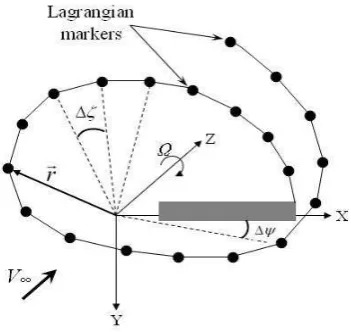
It is assumed that the flow field is incompressible and potential in the free vortex wake (FVW) model for the wind turbine. The blade is modeled as a series of elements, which are represented as a line of bound vorticity lying along the blade quarter chord line. The vertical filaments, extending downstream from the trailing edge of the blade element boundary, are allowed to freely distort under the influence of local velocity field. The governing equation of the vertical filaments can be written in the form of a partial differential equation as

(1)

[image:3.595.211.387.517.683.2]

where the blade azimuth angle is a temporal coordinate and the wake age angle is a spatial coordinate. On the right hand side of Eq. 1, equals to the mean value of the induced velocities at the surrounding four grid points calculated by the Biot-Savart law. To solve the partial differential equation numerically, the finite difference approximations are used to approximate the derivatives on the left hand side. For the spatial ( ) derivative, a five-point central difference approximation has been used based on the PCC Corrector Central difference) [15] and the PC2B (Predictor-Corrector 2nd Backward) [16]. The accuracy of the temporal ( ) derivative approximation plays a significant role in the time-accurate free vortex method. The PC2B algorithm used a second-order backward difference approximation, whereas the PCC algorithm still used a five-point central difference approximation.

Figure 1 Schematic of the discretized tip vortex geometry

In the present work, a new time-accurate algorithm is developed for overall convergence in the numerical iterations. For this, the Eq. 1 can be written in another form as

The Eq.2 can be written in a general form of ordinary derivative equation as

(3)

The predictor process in the predictor-corrector algorithm adopts an explicit format, whereas the corrector process adopts an implicit format. Assuming the steps are equal, the general form of the linear multistep method for Eq.3 is written as

where and represent the terms of and ,respectively. The values of constants and can be obtained using the method of undetermined coefficients. An explicit three-step linear multistep method is given by



2 1



2

3

3

6

3

2

1

 









n



n



n



n

n

y

y

y

hf

y

(5) The local truncation error of Eq. 5 is

 4

_{ }

 

6 4 3

2

1

h

O

x

y

h

T

_n



_n



(6)

An implicit three-step linear multistep method is given by



2 1



3

3

11

6

2

9

18

11

1

  





n



n



n



n

n

y

y

y

hf

y

(7)

The local truncation error of Eq. 7 is

 4

_{ }

 

6 4 3

2

3

h

O

x

y

h

T

n





n



(8)

The explicit and implicit three-step linear multistep methods are used in the temporal (



) derivative approximation. A new predictor-corrector algorithm is developed as:

for the predictor : (9

)

and

_{�nd �nd �nd �nd}

(10)

for the Corrector.

It is obvious from the local truncation errors of Eq.5andEq.7 that the new predictor-corrector algorithm has third-order accuracy, and therefore this algorithm is referred as the D3PC (Three-step and Third-order Predictor-Corrector) algorithm. The PCC is a single-step algorithm and has second-order accuracy. The single-step algorithm is simple, but its numerical stability is not good enough. The multistep method has recently been widely used since it has better stability and convergence. Although the PC3B algorithm is a three-step algorithm, it only achieves second-order accuracy, which results in low efficiency. The D3PC algorithm developed in this paper is also a three-step algorithm, but is of third-order accuracy.

The Three-dimensional rotational effect is one of the typical differences between rotating rotor and fixed wing, resulting in stall delay, which is characterised by significantly increased lift coefficient compared to the corresponding 2D case, and by a delay of the occurrence of flow separation to higher angles of attack. Du-Selig stall-delay model [7]0, which is coupled into the free vortex wake model, is used to modify the airfoil aerodynamic data by consideration of the three-dimensional rotational effect in this work.

The aerodynamic loading is caused by the flow past the wind turbine structure composed of the blades and the tower. The air loads can be calculated through the discrete blade element method. Every blade element is regarded as a 2-D airfoil, and the relative velocity vector is obtained from:

rel







rot



ind



b

V

V

V

V

V

₍₁₁₎

is the rotational velocity. The induced velocity can directly be computed in the free vortex wake method. In the case of an aero elastic computation, it is necessary to calculate the blade elastic deformations denoted by the local blade velocity .

3.

Dynamics equation for aero-dynamic and structural coupling

If a wind turbine is described as a discretized mechanical system, the principle work is to correctly set up the mass matrix, [M], stiffness matrix, [K], and damping matrix, [C], for the dynamics equation:

[M]{ } [ ]{ } [ ]{ }x  C x  K x { ( )}F t (12)

where{ ( )}F t denotes the generalized force vector associated with the external loads.

x

is the

generalized displacement. In the paper, the Newmark method is used to solve the dynamics equation. The discretized calculation process to solve the dynamics equation is presented as:

2

1 1

2

([

]

[ ]

[

]){ }

{ }

[ ]({ } (1

)

{ } )

[

]({ }

{ }

(1 2 ){ } )

2

n

n n

n n n

M

t C

t K

x

F

C

x

t x

t

K

x

t x

x









 

 

 





  





 





(13)

where the subscript represents the time-step number. The displacements at the time step n are calculated from the results of the previous time step , at which the displacements, velocities, and accelerations for each node are already known.

The generalized displacement and velocity in the form of expansion from the time step to the time step n are given by

1 1

1 2

1

{ }

{ }

[(1

){ }

{ }

]

{ }

{ }

{ }

[(1 2 ){ }

2 { }

]

2

n n n n

n n n

n n

x

x

t

x

x

x

x

t x

t

x

x









   



 







 









(14) where



0.5 and



0.25 are the trapezoidal conditions in order to guarantee unconditional

[image:6.595.199.401.75.222.2]

Figure 2 Calculation procedures for dynamic responses

The blade gravitational force and centrifugal force are included in the calculation. Gravity is responsible for a sinusoidal loading of the blades with a frequency corresponding to the rotation of the rotor. The blade experiences tensile stress and compressive stress because of the gravitational loads, thus resulting the blade vibration deformation and affecting the rotor aerodynamic performance. The gravitational loading is obtained from

[0 0

]

T

g i

df



A

m g

(15)

Where is the coordinate system transformation matrix, is the ith blade element mass. is the gravitational loading of the ith blade element.

The inertial loading stems from the centrifugal force on the blades due to rotation. The centrifugal force acting on the blade element at a radiusr from the rotational axis is obtained

from

(16)

4.

The numerical result and analysis

4.1

The calculation model validation

The NREL (National Renewable Energy Laboratory) Phase VI rotor geometry, aerodynamic and structural properties are well documented in the literature[18].The operating condition for the

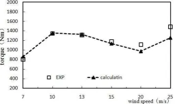
experiment was varied from wind speed of 7 to 25m/s. The rotor speed is 72 r/m, with the tip pitch is 3 degrees and 0-degree cone angle. The rotor radius is 5.029m.

Figure 3 shows variation of rotor torque with wind speed, and compare with the experiment data. The calculation results are found to be in good agreement with the experimental data at low wind speeds. At higher wind speeds, however, there are discrepancies, probably due to the stall

[image:6.595.209.389.642.749.2]

effects.

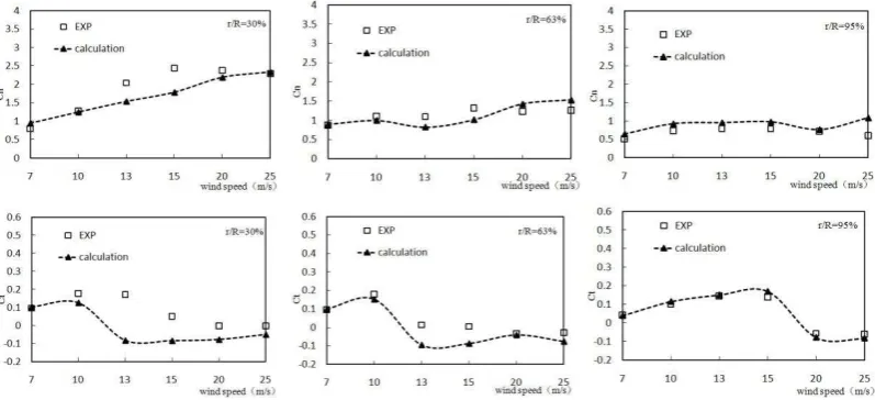
Figure 4 shows the variation of normal and tangential coefficient at different span with wind

speed. Ranging from low to high wind speed, it is found that the normal and tangential force coefficients of the blade root are slightly worse than other part of the blade, which is reason that the

blade root suffers the serious stall effect. It is difficult to simulate the stall situation. The better stall model is needed to use in the free wake method. However, the middle and tip part of blade all have a good match with the experimental data. Therefore, in the paper the calculation model is well used

[image:7.595.94.493.185.367.2]

to calculation the loads of the wind turbine.

Figure 4 Variation of normal and tangential coefficient at different span with wind speed

4.2

The large-scale wind turbine numerical results and analysis

In the paper, the NH1500 wind turbine is adopted as a calculation example. The calculation

time step is10 /. The wind speed is 8m/s. In order to reflect the similarity of NH1500 and real

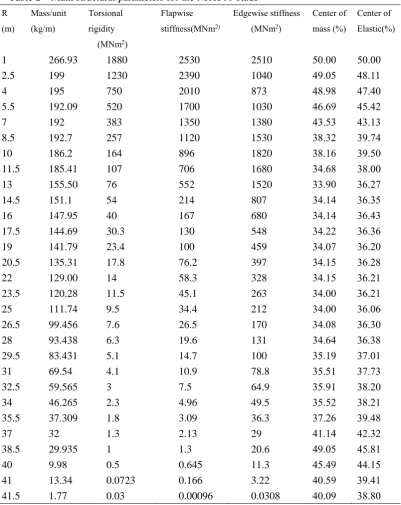
1.5MW wind turbine, the rotor main parameters are shown in Table 1. From the table, it can be seem

that the rated power of NH1500 is 1.5MW. At the same times, the NH1500 and real 1.5MW wind turbine have the similar blade length and wind speed operational condition. And the NH1500 also adopt the variable-pitch variable speed control strategy. Moreover, to more describe the NH1500,

the NH1500 blade main structural parameters are shown in Table 2. The all aerodynamic centers of blade are located in a quarter chord length. Mass and elastic centers are given though chord length

percentage in the airfoil coordinates.

In the paper, the finite element method is applied to establish the wind turbine structural model. Two-node beams and shell elements are used to model the blade and tower, respectively. The nacelle

mass and moment of inertia are simulated through the 0D element in PATRAN software. The rotor is rigidly connected to the tower. The boundary conditions are imposed at the bottom of the tower

[image:7.595.203.396.661.776.2]

through fixed constraints. The modes of NH1500 wind turbine are calculated at the rotational speed of 17.2 rpm with the calculated modes shown in Table 3.

Table 3 The mode description

Mode description Natural frequency(Hz)

Left-righttower1st _0.420

Fore-aft tower 1st _0.422

Blade flapwise 1st _0.775

0.802 0.833

1.335 1.361

Blade flapwise2st _2.049

2.194

[image:8.595.98.498.147.370.2]

2.308

Figure 5 shows the comparison of calculated value and experimental value. NH1500 is a 1/16 scaled model on the experiment. The calculated value and experimental value trend is basically consistent. As can be seen from the figure 5, the calculation values are slightly higher than the

[image:8.595.204.398.212.368.2]

experiment data. It is probable reason that the experiment wind turbine model is scaled model.

Figure 5 Cp of the NH1500

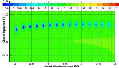
Figure 6 shows the downstream displacements of the blade tip vortex, calculated from the FVW

method. In order to investigate the blade deformation effect, the NH1500 blade is considered rigid and flexible, respectively. Clearly seen from the figures the difference in the vortex position between the assumed rigid blade and the actual flexible blade. The displacement difference increases from

0.05R to 0.1R as the tip vortex filament moves down stream. It can be reasoned that this difference has influence on the air load calculation through the induced velocity calculation, which depends

the spatial distance of the vortex to the blade.

For further analysis, the wind speed distribution and the vorticity of the wake are calculated in

the paper. The wind speed of the wake

V V V V

(

x

,

y

,

z

)

is defined as

( ,

_{x y}

,

_z

)

_indtip _indb _indt _inds

V V V V



V



V



V



V



V



(17)

To find the wind speed of the wake seen by the

V V V V

(

x

,

y

,

z

)

, the induced velocity of the tip

vortex ,

V

_indtip, the induced velocity of the bound vortex,

V

_indb , the induced velocity of the trailed vortex,

V

_indt , the induced velocity of the shed vortex,

V

_inds , must be added as vectors to the inflow velocity,

V

_.

After the wind speed distribution is known, the vorticity

   

( ,

x y

,

z

)

is calculated by: y

z x

x z

y

y x

z

V

V

y

z

V

V

z

x

V

V

x

y



















_

_





_



_





_

_







_

_





_

_

[image:8.595.250.329.635.734.2]



₍₁₈₎

Figure 7 and Figure 8 give the development and evolvement of the tip vortex for the rigid and

downstream just behind the rotor with a wake expansion, but gradually dissipates as the axial

[image:9.595.211.379.128.252.2]

distance further increases for the both cases. However, both the vortical strength and the wake expansion for the assumed rigid rotor are stronger than those for the actual flexible rotor.

[image:9.595.201.396.285.392.2]

Figure 6 Cyclic variation of the tip vortices with downstream distance

Figure 7 Axial distribution of the tip vortex for the rigid blade

Figure 8 Axial distribution of the tip vortex for the flexible blade

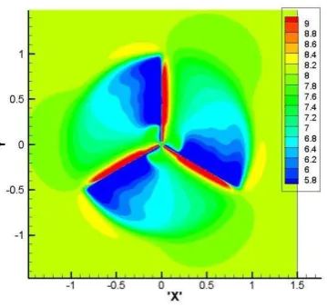
[image:9.595.199.393.424.535.2] [image:9.595.210.388.561.723.2]

[image:10.595.210.390.73.242.2]

Figure 10 0R section distribution of the wind speed

V

_z(m/s) of the flexible blade Figure 9 shows the 0R section distribution of the wind speed of the rigid blade. Figure 10 shows the0R section distribution of the wind speed of the flexible blade. Through the two figures, it is

found that the 0R section wind speeds of the flexible blade are weaker than the rigid due to the structural deformation. The effect is significant for wake prediction.

Figure 11 shows some representative numerical results in which the aerodynamic

characteristics are presented by the blade root loads for the flexible case at the wind of 8m/s. The root loads all fluctuate sinusoid ally with azimuthally angle for both the cases of gravity considered

and gravity not considered, but the amplitude of the load variation is greatly different each other due to the gravitational effect. In addition, the blade dynamic deformation is also influenced by the gravity. The dynamic displacement in the flapwise direction when the gravitational force is not

considered is about only 4%of that when the gravitational force is taken into account, as shown in Figure 12.

a) without gravity b) with gravity

Figure 11 Edgewise force at blade root

[image:10.595.91.487.445.706.2]

[image:11.595.198.394.73.188.2]

Figure 13 Wind turbine power coefficients,V_8 /m s

It is obvious from Figure 13, where the wind turbine power coefficient Cp is compared between the rigid and flexible considerations, that the flexible wind turbine Cp is larger than the rigid one

and changed with azimuth angle. According to the comparison of minimum value, the flexible wind turbine Cp is more 1.6% than the rigid one. It is the reason that the flapwise direction induced

velocity of flexible blade has greater change than the edgewise direction induced velocity. And the flapwise direction induced velocity is weaker than the rigid one. Thus, the attack angle and the flow

angle of flexible blade are all larger. Finally, the tangential force coefficient to the rotor is larger, which can lead to the increasing of torque and Cp.

5.

Conclusions

The numerical analysis of wind turbine wake and loads are presented in this paper. An aerodynamically and structurally coupled model is developed and used to predict the flexible wind turbine loads and aerodynamic performance. The results demonstrate that the FVW and FEM coupling model can predict the wind turbine dynamic characteristics effectively and efficiently. The dynamic displacement in the flapwise direction when the gravitational force is not considered is only 4% of that when the gravitational force is taken into account. Moreover, according to the comparison of minimum value of what???, the Cp value of the flexible wind turbine is more 1.6% than that of the rigid one. Despite the accuracy of calculated results will need to be improved for further validation by experiment data, the wind turbine wake and dynamic response can be better understood through the results obtained from this study.

Reference

[1] Ghadirian A., Dehghan, M., Torabi, F.. Considering induction factor using BEM method in wind farm layout optimization [ J]. 2014,129:31-39.

[2] Zhang Zhenyu, Zhou Hanwei, Wangtongguang. Numerical Analysis of Influence of Gurney

Flaps Applied to Wind Turbines. Transactions of Nanjing University of Aeronautics &

Astronautics[J]. 2014,31(5): 576–579.

[3] Ming Chen Hsu, Ido Akkerman and Yuri Bazilevs. Finite element simulation of wind turbine aerodynamics: validation study using NREL Phase VI experiment[J]. Wind Energy,

2014,17:461-481.

[4]F. Grasso, A. van Garrel, G. Schepers. Development and Validation of Generalized Lifting Line

Based Code for wind turbine Aerodynamics[C]. The 30th ASME wind energy symposium, Florida. 2011:146-152.

[5]Frank Scheurich, Timonthy M. Fletcher, Richard E. Brown. Simulating the aerodynamic

[6] Breton SP, Coton FN, Moe G. A study on rotational effects and different stall delay models

using a prescribed wake vortex scheme and NREL phase VI experiment data. Wind Energy, 2008, 11: 459–482.

[7] Wang T G. Unsteady Aerodynamic Modelling of Horizontal Axis Wind Turbine Performance[D]. PhD Dissertation, University of Glasgow. November 1999.

[8] Sebastian T, Lackner MA. Development of a free vortex wake method code for offshore floating

wind turbines [J]. Renewable Energy, 2012, 46: 269-275.

[9] Zhou WP, Tang SL, Lü H, Computation on aerodynamic performance of horizontal axis wind

turbine based on time-marching free vortex method [J]. Chin.Soc.for Elec.Eng., 2011, 31(29):124-130.

[10] Jeon M, Lee S. Unsteady aerodynamics of offshore floating wind turbines in platform pitching

motion using vortex lattice method [J]. Renewable Energy, 2014, 65: 207-212.

[11] Gupta S, Leishman JG. Performance Pre-dictions of The NREL Phase Combined

Ex-periment Rotor Using a Free-Vortex Wake Model[C]. Collection of Technical Papers-44th AIAA Aerospace Sciences Meeting. 2006:4544-4564.

[12] Eelco H, Gustaaf . J, Asfaw B. Aero-elastic behavior of a flexible blade for wind turbine

application: A 2D computational study[J]. Energy, 2010;35:778–785.

[13] Anders Ahlstrom. Aeroelastic Simulation of Wind Turbine Dynamics[D]. Doctoral Thesis from

Royal Institute of Technology Department of Mechanics. Sweden. April 2005.

[14] Bing Feng Ng, Henrik Hesse, Rafael Palacios. Aeroservoelastic state space vortex lattice

modeling and load alleviation of wind turbine blades[J]. wind energy. 2014:DOI: 10.1002/we.1752.

[15] Bhagwat MJ, Leishman JG. Rotor Aerody-namics During Maneuvering Flight Usinga Time-Accurate Free vortex Wake [J]. Journal of the American Helicopter Society, 2003;48:143-158.

[16] Bhagwat MJ, Leishman JG. Time-accurate free vortex wake model for dynamic rotor response[C]. American Helicopter Society Specialist Meeting. Atlanta, 2000.

[17] Du Z, Selig MS. A 3-D Stall-Delay Model for Horizontal Axis Wind Turbine Performance

Prediction[R]. AIAA-98-0021, 1998.

[18] Hand M, Simms D A. Unsteady aerodynamic experiment phase VI wind tunnel test

configurations and available data campaigns[R] National Renewable Energy

[image:12.595.92.299.564.691.2]

Laboratory Colorado National Technical Information Service 2001.

Table 1 the NH1500 rotor parameters

Number of blades 3

Rotor radius 41.5m

Blade length 40.5m

Rated rotational speed 17.25rpm

Rated power 1.5MW

Rated wind speed 10.5m/s

Cut-in wind speed 3m/s

Table 2 Main structural parameters for the NH1500 blade

R

(m)

Mass/unit

(kg/m)

Torsional

rigidity

(MNm2₎

Flapwise

stiffness(MNm2)

Edgewise stiffness

(MNm2₎

Center of

mass (%)

Center of

Elastic(%)

1 266.93 1880 2530 2510 50.00 50.00

2.5 199 1230 2390 1040 49.05 48.11

4 195 750 2010 873 48.98 47.40

5.5 192.09 520 1700 1030 46.69 45.42

7 192 383 1350 1380 43.53 43.13

8.5 192.7 257 1120 1530 38.32 39.74

10 186.2 164 896 1820 38.16 39.50

11.5 185.41 107 706 1680 34.68 38.00

13 155.50 76 552 1520 33.90 36.27

14.5 151.1 54 214 807 34.14 36.35

16 147.95 40 167 680 34.14 36.43

17.5 144.69 30.3 130 548 34.22 36.36

19 141.79 23.4 100 459 34.07 36.20

20.5 135.31 17.8 76.2 397 34.15 36.28

22 129.00 14 58.3 328 34.15 36.21

23.5 120.28 11.5 45.1 263 34.00 36.21

25 111.74 9.5 34.4 212 34.00 36.06

26.5 99.456 7.6 26.5 170 34.08 36.30

28 93.438 6.3 19.6 131 34.64 36.38

29.5 83.431 5.1 14.7 100 35.19 37.01

31 69.54 4.1 10.9 78.8 35.51 37.73

32.5 59.565 3 7.5 64.9 35.91 38.20

34 46.265 2.3 4.96 49.5 35.52 38.21

35.5 37.309 1.8 3.09 36.3 37.26 39.48

37 32 1.3 2.13 29 41.14 42.32

38.5 29.935 1 1.3 20.6 49.05 45.81

40 9.98 0.5 0.645 11.3 45.49 44.15

41 13.34 0.0723 0.166 3.22 40.59 39.41

[image:13.595.99.501.83.589.2]