The Development of Web-Based Interface to Census Interaction Data

This is a repository copy of The Development of Web-Based Interface to Census Interaction Data.

White Rose Research Online URL for this paper: http://eprints.whiterose.ac.uk/5024/

Monograph:

Stillwell, J. and Duke-Williams, O. (2000) The Development of Web-Based Interface to Census Interaction Data. Working Paper. School of Geography , University of Leeds. School of Geography Working Paper 00/04

[email protected]

Reuse

Unless indicated otherwise, fulltext items are protected by copyright with all rights reserved. The copyright exception in section 29 of the Copyright, Designs and Patents Act 1988 allows the making of a single copy solely for the purpose of non-commercial research or private study within the limits of fair dealing. The publisher or other rights-holder may allow further reproduction and re-use of this version - refer to the White Rose Research Online record for this item. Where records identify the publisher as the copyright holder, users can verify any specific terms of use on the publisher’s website.

Takedown

If you consider content in White Rose Research Online to be in breach of UK law, please notify us by

WORKING PAPER 00/04

The Development of a Web-based Interface to

Census Interaction Data

John Stillwell and Oliver Duke-Williams Centre for Computational Geography,

School of Geography, University of Leeds,

Leeds LS2 9JT [email protected] [email protected]

TABLE OF CONTENTS

Page

CONTENTS iii

LIST OF TABLES iv

LIST OF FIGURES iv

ABSTRACT v

1. INTRODUCTION 1

2. OBJECTIVES AND REQUIREMENTS 2

3. INTERACTION DATA SETS 6

3.1 1991 Special Migration Statistics 6

3.2 1991 Special Workplace Statistics 10

3.3 1981 Special Migration Statistics 11

3.4 1981 Special Workplace Statistics 14

3.5 Studies using the SMS and SWS 15

4. SYSTEM ARCHITECTURE 16

4.1 Overcoming the Limitations of the Web 16

4.2 Dynamic Web Pages 17

4.3 Maintaining State 19

4.4 Database Uses 20

4.5 Overview of system architecture 21

4.6 Provision of Advanced Features 22

4.7 Use of metadata 25

5. USING THE INTERFACE 44

5.1 Login and the General User Interface 44

5.2 Selection of geographical areas 45

5.3 Selection of Variables 50

5.4 Extraction and Output 51

6. 2001 CENSUS INTERACTION DATA 59

7. CONCLUSIONS 63

LIST OF TABLES

Page

1. Fields in 'meta_datasets' and their uses 27

2. Sample entries for fields in 'meta_datasets' for 1991 SMS Set 1 29

3. Fields in 'meta_tables' and their uses 31

4. Sample entries for fields in 'meta_tables' for Tables 1 and 2 of the 1991 SMS Set 1

31 5. Basic layout of the table defined in Table 4, sample record 1 32 6. Basic layout of the table defined in Table 4, sample record 2 33

7. Fields in 'meta_vars' and their uses 34

8. Fields in 'meta_geog' and their uses 36

9. Sample entry in 'meta_geog' 37

10. Fields in 'meta_geoglut' and their uses 39

11. Part of the ddatabase table lut_gbward 1991 39

12. Fields in 'meta_users' and their uses 41

13. Fields in 'meta_dataperms' and their uses 43

14. Fields in 'meta_usage' and their uses 43

LIST OF FIGURES

1. Examples of using PHP and HTML to write messages 19

2. WICID system architecture 24

3. Metadata structure 28

4. WICID Login Screen 47

5. WICID Welcome Screen 47

6. WICID General Query Interface 48

7. WICID Geographical Area Status 48

8. WICID Area Selection Tools 49

9. WICID List Selection of Countries 49

10. WICID Flow Type Selection 52

11. WICID Data Selection Tools 52

12. WICID Data Set Selection 53

13. WICID Table Selection 53

14. WICID Variable Selection 54

15. WICID Query Completed 54

16. WICID Simple Query 55

17. WICID More Complex Query 55

18. WICID Output Selection 57

19. WICID Labels Selection 57

20. WICID Output Preview 58

ABSTRACT

1 Introduction

Successive censuses since 1961 in Great Britain have asked respondents questions about their change of usual residence and their daily commuting behaviour. Much of the data collected on interaction flows in recent censuses have been incorporated into various published census products such as the National and Regional Migration Reports or the Workplace and Transport to Work Reports. It was not until the 1981 Census that the Special Migration Statistics (SMS) and the Special Workplace Statistics (SWS) produced by OPCS were purchased by the ESRC on behalf of the academic community. Equivalent data sets were obtained in 1991 and it is proposed that sets of origin-destination statistics will be produced from the 2001 Census.

Despite their perceived importance and potential, the SMS and SWS are census products that have been underused by researchers and planners hitherto. Both data sets are large and complex and their use has been constrained for two reasons in particular: limitations associated with the flows available in the data sets and difficulties associated with data extraction. The overall aim of this Census Development Programme project is associated with the latter problem and thus to increase the use of the special migration and commuting data that will be produced from the 2001 Census.

This paper describes the progress that has been made on the development of an Internet-based software system to access data from previous censuses. The paper contains a summary of the data sets involved and a short review of their use in academic studies (Section 3). An outline of the system architecture and of the structure of the metadata required to develop the information system is presented (Section 4) and the process of building a query to extract data is exemplified using a sequence of Web pages (Section 5). A short summary of the proposed tabulations for 2001 is also included (Section 6). We begin, however, by presenting the specific objectives and the requirements of the system in the next section.

2 Objectives and Requirements

The project has the following objectives:

to provide users with access to SMS and SWS data via the Internet; to develop an easy to use interface for data extraction;

to generate a library of popular sub-sets of interaction data;

The size and complexity of the SMS and SWS origin-destination data sets present a considerable challenge to users wishing to undertake computer-based analyses of migration and commuting patterns. Various software systems have been developed in the past. MATPAC was developed to handle the 1981 Census data whereas a choice of software systems has been available for users to extract 1991 SMS and SWS interaction data via MIDAS (subsequently MIMAS). SMSTAB is the software developed initially at the University of Leeds by Oliver Duke-Williams and made available via MIDAS for use by academics to access the SMS data. SMSTAB was converted into SWSTAB to provide access to the SWS Set C. QUANVERT is the alternative software platform for providing flexible and rapid access to the SMS and SWS Set C. SMSTAB and SWSTAB both operate through preparing files containing sets of line commands. QUANVERT is a commercial product that has been adapted to do much the same task.

not in such a way as to over-complicate the procedures involved. In fact, a key principle is to minimise the information and parameters that are required in building an extraction query which might then be run either online or in batch mode.

Interaction flow data is unlike stock data in that it is not possible to simply add the total outflows from one area to the total outflows from a neighbouring area to give an aggregate total. Flow data is non-additative because of the need to remove the flows taking place between the two areas that are included in the respective totals. Given this problem, one of the most challenging requirements is to develop a system that allows for the flexible aggregation of origin and destination areas. Such a facility is very useful because it enables users to extract detailed spatial information for small areas in which they may have a particular interest whilst simultaneously generating interaction flows for larger areas that are of less direct importance but may provide valuable contextual or comparative information. For example, a user may be particularly interested in the flows between wards of a major city, but may also wish to generate aggregate flows between each ward and the surrounding districts as well as flows from each ward to other regions throughout GB. Allowing flexibility in the specification of both the origin and destination geographies means that it becomes possible to close the system or to account for the remaining flows. However, it is necessary to incorporate some limitations on the number of geographical scales at which area aggregation is feasible.

examples of flow matrices likely to be popular amongst users. The intention is to use the WICID system to create and validate a limited number of popular data sub-sets that would then be available directly from a library. Downloading files would take a minimum of mouse clicks. Access to the queries used to extract the data would also be available to users to check the precise specifications of the data. The library facility would be expanded when appropriate to allow users to deposit new sub-sets of data and the associated queries.

Whilst accurate data extraction is the predominant function of the WICID system, users of migration and commuting data often require raw census data to be manipulated in some way before being interpreted, analysed or visualised. Consequently, one of the objectives of the project is to provide, as a set of options, some data manipulation or analytical functionality. On the one hand, this will involve the provision of a set of tools for ranking and sorting the data and the computation of some simple descriptive statistics (e.g. mean, standard deviation, maximum, minimum, range) for the sub-set of flows extracted. On the other hand, we envisage the need to provide tools to derive new variables based on the data extracted (e.g. net migration or migration efficiency) or requiring other information such as populations (e.g. migration intensities, commuting velocities). The second requirement implies the storage in the database of appropriate populations at risk for use as denominators as well as careful explanation of the ways in which new variables are derived.

2001 Census when they become available. Work up to the present time has focused on building a system that provides access to the 1991 Census SMS and SWS. However, a further objective of the project is to provide access to other interaction data sets relating to both the 1991 and 1981 Censuses, details of which are outlined in the next section.

3 Interaction Data Sets

3.1 1991 Special Migration Statistics

The 1991 SMS are a set of statistics relating to the characteristics of individual migrants or migrant households in the 12 month period preceding the 1991 Census. A migrant is defined as a resident who has a different usual address one year before the Census to that at the time of the Census. A wholly moving household, as the name implies, is a household where all the usually resident members aged one and over are migrants. Full details of the organisation and content of the SMS are given in OPCS and GRO(S) (1993a, 1993c) and have been summarised by Flowerdew and Green (1993). Two sets of 1991 SMS were created:

SMS Set 1 provides migration flow statistics for wards (England and Wales)

and postcode sectors (Scotland); and

SMS Set 2 provides migration flow statistics for districts in Great Britain.

120 million potential flows. In fact, the SMS 1 matrices are quite sparsely populated as only a small percentage of the potential number of origin-destination pairs have flows associated with them. For example, only about 1% of the potential number of origin-destination pairs in Great Britain in SMS 1 were non-zero (Cole, 1995). The SMS 1 involve two tables containing 12 counts or variables:

Table 1: All migrants: age by sex (five broad age groups) (10 counts); and Table 2: Wholly moving households and residents in them (2 counts).

The SMS 2 data set consists of counts associated with the migration flows between the districts of Great Britain. There are 459 districts involved (366 in England, 37 in Wales and 56 in Scotland). In addition, flows from foreign countries to districts in Great Britain are included. Associated with each flow is a variable number of counts: the data given in SMS 1, together with more detailed socio-economic details about migrants when a suppression threshold permits. The SMS 2 comprises 12 tables containing 93 counts:

Table 1: All migrants: age (5 broad age groups) by sex (10 counts); Table 2: Wholly moving households and residents in wholly moving

households: counts (2 counts);

Table 3: All migrants: age (5 year groups) by sex (38 counts); Table 4: All migrants: marital status by sex (6 counts);

Table 5: All migrants: ethnic group (4 counts);

Table 6: All migrants: whether resident in households by whether suffering

Table 7: All migrants aged 16+: economic position (7 counts); Table 8: Wholly moving households: tenure (3 counts);

Table 8S: Wholly moving households: tenure (4 counts);

Table 9: Wholly moving households: sex and economic position of head (7

counts);

Table 10: Residents in wholly moving households: sex and economic position

of head (7 counts);

Table 11S: All migrants: Gaelic speakers (1 count); and Table 11W: All migrants: Welsh speakers (1 count).

Details of the SMS are outlined in Rees and Duke-Williams (1994, 1995). The SMS data are derived from the 100% sample and include imputed households. Unlike the published Migration Topic Reports (OPCS 1994), no 10% variables (e.g., social class/SEG, industry or occupation) are available. For reasons of privacy and confidentiality, migrant data in SMS 2 are suppressed when there is a flow of less than 10 people between two districts, and details of wholly moving households are suppressed when there are less than 10 households in a given flow. In addition, details are suppressed when there are 10 or more migrants, but all of them members of the same (wholly moving) household. The suppression thresholds used mean that a large amount of the potential data in SMS 2 is not released. Rees and Duke-Williams (1995) have investigated the problem of suppression and have identified the total extent of the problem as involving:

flows between 135,916 origin-destination pairs of districts suppressed

flows between 110,268 origin-destination pairs of districts suppressed

because there are less than 10 wholly moving households; and

the flow from Havering in Greater London to Carmarthen in Dyfed which

involved more than 10 migrants but all were part of the same (wholly moving) household.

Rees and Duke-Williams (1997) have estimated the data for suppressed flows in Tables 3-10.

Simpson and Middleton (1999) subsequently looked at the impact of the 2% underenumeration in the 1991 Census and identified three further elements ‘missing’ from the SMS data in addition to the suppressed (unpublished) flows. These are due to:

unit-response - migrants among 1.2 million unrecorded residents - estimated to

be between 218,000 and 376,000 individuals;

item non-response - residents who were recorded as migrants in the Census

but with origin unknown - 326,000 migrants had origins unknown; and

reporting error - those residents who were recorded in the Census but whose

migrant status was wrongly recorded - approximately 500,000 people.

Middleton was to add 10% to all flows as an allowance for the net impact of mis-reporting of migrants as measured in the Census quality check. This adjustment is not included in the tables reported in the published paper since the authors recognised that the equal enlargement of every flow might be misleading.

WICID will provide users with access to the adjusted data sets from the respective tables in SMS 2 as well as the raw data in each of the tables in the SMS 1 and 2. An option will be available of adding 10% to the SMS 2 Table 3 counts adjusted by Simpson and Middleton. Permission will be sought from ONS/GRO(S) to provide a sample set of aggregate data, blurred to preserve confidentiality, that will be available unregistered users who want to explore how the information system operates.

3.2 1991 Special Workplace Statistics

Table 1: Economic position and age: employees and self employed (54

counts);

Table 2(1): Hours worked (10 counts); Table 2(2): Family position (12 counts);

Table 4: Distance to work: employees and self employed with workplace

coded (16 counts);

Table 5: Transport to work: employees and self employed (22 counts); Table 6: Cars available in households: employees and self employed in

households (10 counts);

Table 7: Occupation (sub-major groups): employees and self employed

(48 counts);

Table 8: Social class and socio-economic group: employees and self employed

(54 counts); and

Table 9: Industry divisions: employees and self employed (48 counts).

Since the data were obtained from a 10% sample, problems of adjustment to preserve confidentiality are not encountered in the SWS and users will have access to the raw counts in each of the tables through WICID.

3.3 1981 Special Migration Statistics

wards and to higher level geographies for publication in printed reports. Ballard and Norris (1983) indicate that between 1 and 2% of addresses were referenced to an incorrect ward.

The 1981 SMS are also divided into two sets. Set 1 is comprised of 148 cell counts for both individual and household-based units for one-year migrants in six tables. The four tables based on 100% counts of individual migrants are as follows:

Table 1: Migrants usually resident/formerly resident by ward aged 16 and over

by economic position and sex (16 counts);

Table 2: Migrants in private households usually resident/formerly resident by

ward aged 16 and over by economic position by household tenure and sex (44 counts);

Table 3: Migrants usually resident/formerly resident by ward by marital status

and sex (8 counts); and

Table 4: Migrants usually resident/formerly resident by ward by age and sex

(36 counts).

The two tables based on wholly moving households or persons in them are as follows:

Table 5: Wholly moving households within/into/from each ward by economic

position by age of head of household (32 counts); and

Table 6: Persons in wholly moving usually resident/formerly resident by ward

Five types of migration data were available from SMS Set 1 in principle: flows within each ward; flows from each ward to each district; flows from each district to each ward; flows from outside Great Britain to each ward; and flows from origin ‘not stated’ to each ward. This basic structure appeared straightforward but, as Cole and Squires (1987) have indicated, confidentiality constraints imposed a more complex structure on the data set. The critical constraint was that if the number of migrants in any one of these categories fails to reach 25, the flow may be ‘thresholded’ up into the next highest geographical level. Thus, a flow of 20 migrants within a ward, for example, may become part of a flow from the ward to a district or county remainder. This ‘cascading’ of flow data presents significant complications when attempting to extract meaningful information from the data set and to examine the pattern and structure of migration flows into and out of districts. For these reasons, Cole and Squires suggested that the SMS Set 1 was a very limited data set for conducting detailed migration research and that the county is the most refined spatial scale at which flows can be considered as reliable. The thresholding problem is the major reason why this data set has received such limited attention.

task is facilitated by the re-tabulation of 1981 migration data for small areas in Scotland in 1991. When the complete national ward-to-ward matrices for males and females have been estimated, the data will be made available through the WICID interface, allowing users to conduct their own analyses of change between 1981 and 1991. It will be possible to re-use the techniques developed for this project when the 2001 origin-destination data sets become available to generate interaction flows for the 1980-81, 1990-91 and 2000-01 for a consistent set of small areas.

3.4 1981 Special Workplace Statistics

Those completing the 1981 Census forms were asked to record the address, with the postcode if known, of the place of work of each person aged 16 or over in a job in the week prior to the Census. A 10% sample of the census forms were taken and workplace postcodes coded and referenced to wards. As in 1991, local workplace statistics for 1981 are in three sets: Set A provides counts of persons aged 16 and over in a job ‘last week’ according to workplace; Set B provides counts of persons aged 16 and over in a job ‘last week’ according to usual residence; and Set C provides counts of trips between usual residence and workplace. Since the data was taken from a 10% sample, there was no need to make further adjustments for confidentiality and the data are not subject to thresholding. Details of the SWS are found in OPCS/GRO(S) (1993c, 1993d).

data in each of these tables that will be re-estimated for 1991 wards in the companion CDP project. Our intention is that, as with the estimated SMS Set 1 data, the re-estimated SWS Set C data will be available to users through WICID.

3.5 Studies using the SMS and SWS

Whilst the SMS and SWS have been used by ONS and in local government for various functions, both sets of data remain under-used in both empirical and modelling migration research. One recent example of empirical work based on 1991 SMS is the updating of The Scottish Office's 1992 study of Scottish Rural Life (Williams et al., 1999). The availability of the SMS allowed a much fuller analysis of migration than in the previous report showing that all of the districts in rural Scotland had net in-migration in the year preceding the 1991 Census. The 1991 SMS have been used to analyse migration patterns in Scotland more generally by Forster (1998), highlighting the fact that different migrant sub-groups, especially different life-cycle groups, have different movement patterns. Earlier, Champion (1994) and Champion and Atkins (1996) used the SMS to analyse migration change in Britain as a whole whilst Flowerdew and Boyle (1992) used the 1981 SMS and SWS to compare inter-ward migration and commuting in Hereford and Worcester.

processes such as suburbanization, counterurbanization, intra-urban mobility, rural depopulation and the relationship between housing and demographic change at the local level. Other examples of the use of the 1991 SMS in modelling work include the application of the Poisson approach to migration flows into the Scottish highlands and islands, from the remainder of Britain, between 1990 and 1991 (Boyle, 1995) and the calibration of spatial interaction models on the entire 1991 SMS Set 1 inter-ward matrix using parallel programmimg techniques on a high performance computer (Turton and Openshaw, 1998).

The use of SWS for academic research appears to be even less than the SMS. Frost et

al. (1996, 1997, 1998) have used the SWS to look at the energy consumption

implications of changing journeys to work in London, Birmingham and Manchester, whilst Spence and Frost (1995) found that the propensity of residents to work locally has marginally fallen over time, but certainly not at a rate that might be expected given the statistics on average work journey lengths.

4 System Architecture

4.1 Overcoming the limitations of the web

This works well for collections of information which will not change, but the model has significant drawbacks: the system is simple, static and stateless.

The system is simple in the sense that the basic interface toolkit provided by HTML – the mark-up language used to write Web pages – is limited. It can be used effectively to display and provide multimedia material, but the elements provided to allow interaction with a user are poor. These elements include buttons and tick boxes, but they are rudimentary when compared to the elements that are typically used when developing a stand-alone program with a graphical interface. The term static means that the files are not modified in any way before being sent back to the client. Any serious application will require output to be dynamic, so that it can be modified to suit the needs of each user. For example, a national Web site giving details of films being shown at local cinemas needs to be able to send details about only those cinemas which are local to each user, rather than simply sending a huge list of all films being shown at all cinemas in the country. Finally, stateless means that all requests from clients are treated independently by the server, regardless of previous pages viewed. In the case of the cinema example, it is necessary to pass data from one Web page (e.g. a search form) about the user’s whereabouts to another Web page (the results page) and thus to maintain state within the server.

4.2 Dynamic Web pages

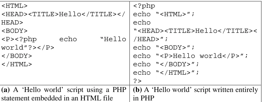
Dynamism is often provided by adding a scripting facility to the Web server. This extends the traditional Web model. When the Web server receives a request for a dynamic page, it can determine that in order to satisfy the request it must run a script (or program). This script will have various inputs (data supplied by the user, such as his or her location) and will generate output that can be understood by the client browser (i.e. in the form of an HTML file). Although the Web server handles requests for dynamic content in a different way, the browser receives the results and displays them in exactly the same fashion.

<HTML>

<HEAD><TITLE>Hello</TITLE></ HEAD>

<BODY>

<P><?php echo “Hello

world”?></P> </BODY> </HTML> <?php echo “<HTML>”; echo “<HEAD><TITLE>Hello</TITLE>< /HEAD>”; echo “<BODY>”;

echo “<P>Hello world</P>”; echo “</BODY>”;

echo “</HTML>”; ?>

(a) A ‘Hello world’ script using a PHP

statement embedded in an HTML file

(b) A ‘Hello world’ script written entirely

in PHP

Figure 1: Examples of using PHP and HTML to write messages

Both scripts in Figure 1 will produce the same output whenever called, and thus do not exhibit any dynamism. However, complex scripts can contain as much program branching, conditional logic and calls to databases as are desired.

4.3 Maintaining state

A server-side language such as PHP can thus produce dynamic Web pages with relative ease. However, the Web model remains stateless. In order to develop a complex application, it is necessary to pass information between pages giving the current state of whatever variables are required to produce the ultimate required output. In an application such as WICID, large amounts of data must be held. With small applications, it is possible to pass information explicitly between different Web pages (for example, coded within a suffix to the web URL); however, as applications become larger, this becomes impractical.

necessary to identify each user (determine who they are), authenticate them (make sure that they are who they say they are) and then keep track of the current state of the application from that user’s perspective. In WICID, this is done with a code library called PHPLIB (http://phplib.netuse.de). This library is written in the PHP language, and contains a series of functions that implement the required session management features. The use of PHP, including features provided by the PHPLIB library, therefore permits the development of a dynamic Web application, in which state can be maintained for the duration of a session. A session begins when a user logs in to the WICID system, and ends either when he/she logs out, or after a certain inactivity time limit has expired.

4.4 Database uses

The general purpose of WICID is to provide access to a large body of data. These data are stored in a database, and the Web interface is intended to help users build a query that will return a subset of data. When the query is ready, it is passed to a DBMS, which processes the query, and sends the results back to the WICID system. The DBMS chosen for WICID is PostgreSQL (http://www.postgresql.org). As the name suggests, the database uses SQL as its query language. The choice of an SQL database is important since this means that it is relatively simple to substitute PostgreSQL with any other SQL-compliant database system.

which the interaction data are coded (e.g. 1991 districts in the case of the 1991 SMS Set 2), and the permissions which are required for a user to be able to access a given data set. The metadata are fully described in Section 4.7. The second additional data set contains those data required to maintain the state of each WICID session. Thus, there is a database table which contains a record for each current session, holding the current values of all session variables. Although the current development version of WICID uses the same DBMS to store a wide variety of data (primary interaction data, supporting metadata and application session data), it is not necessary to use the same DBMS for all these purposes. In fact, there are often advantages to using a different DBMS – perhaps running on different physical machines, in different locations – for different purposes, and thus spreading the computational load more efficiently.

4.5 Overview of system architecture

WICID uses the server-side language PHP, together with the library PHPLIB, to provide dynamic content, in which individual users can generate and execute complex queries. The task of data management and retrieval is carried out by an SQL database management system, PostgreSQL. Figure 2 illustrates this model.

Of course, the PHP scripts which form the application do far more than simply form SQL statements and send them to a DBMS, and may also interact with other programs – the interaction with a DBMS is shown as one example of the function and scope of PHP within the WICID system.

The Web server portion of Figure 2 shows the server retrieving files from a filestore, and either sending them directly back to the user, or onto PHP for processing. This part of the Figure is a simplified view of the system, in order to illustrate this process. In fact, PHP is effectively a part of the Web server (it is one of many modules compiled into the server) rather than an independent entity.

4.6 Provision of advanced features

sophisticated interactive selection tools in the interface, or to incorporate some level of validation of submitted data in order to check for errors.

Results SQL

statements

Output in the

form of a

‘plain’ file Files which

need to be

processed ‘Plain’ HTML etc.

files

Web browser

Web server

Filestore

PHP / PHPLIB

PostgreSQL

Session

state data

Interaction

data

Metadata WEB SERVER USER VIEW

PHP

DBMS

4.7 Use of metadata

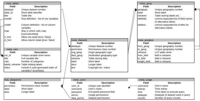
As well as the main migration and commuting data sets, there is also a body of metadata used by WICID. As indicated in Section 4.4, these metadata include information such as the details of the geographies for which the main data sets are coded. This section of the paper describes the general structure of the metadata system in WICID.

observations and must be coded with a unique pairing of origin and destination. However, this rule does not lead to many assumptions within the application code, and could be over-ridden if necessary.

Given the general data structure outlined above, WICID enforces a set of requirements concerning the types of fields used to hold the data, and the names of all fields used in the database. This is done so that the name of any field can be derived internally wherever needed using a fixed set of rules. Data to be loaded into the system must therefore be coded appropriately and all fields given their ‘correct’ names.

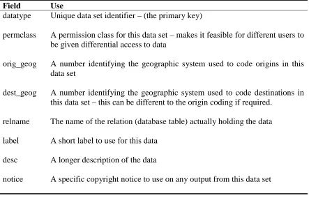
Table 1: Fields in ‘meta_datasets’ and their uses

Field Use

datatype Unique data set identifier – (the primary key)

permclass A permission class for this data set – makes it feasible for different users to be given differential access to data

orig_geog A number identifying the geographic system used to code origins in this data set

dest_geog A number identifying the geographic system used to code destinations in this data set – this can be different to the origin coding if required.

relname The name of the relation (database table) actually holding the data label A short label to use for this data

desc A longer description of the data

meta_tables meta_geog

Field Description Field Description

datatype Unique dataset number geogtype Unique geography number

table_id Short table identifier label Short label

title Table title relname Table storing labels etc.

rowdef Row definition - list of row variables labfields comma separated list of field names

of alternative labels coldef Column definition - list of column

variables

labdesc comma separated list of titles for alternative labels

map Way in which cells map: [row/col/colskip]

rt_hint Allow row totals [true / false]

ct_hint Allow column totals [true / false] meta_datasets meta_geogluts

Field Description Field Description

datatype Unique dataset number from_geog Unique geography number

meta_vars permclass Permissions class number to_geog Unique geography number

Field Description orig_geog Origin geography type relname LUT table name

var_id Unique variable short name dest_geog Destination geography type from_field field in relname

title Full variable title relname Table storing data to_field field in relname

cats Number of categories label Short label weight_field field in relname

labels_relname Table holding labels desc Longer label index Include in auto-generated index of

variables? [true/false]

text Copyright etc. notice

meta_dataperms meta_users meta_usage

Field Description Field Description Field Description

permclass Permissions class number user_id Unique user identifier username User's name

label Short label username User's name tstamp Time stamp

desc Longer label password Encrypted password field time Time taken to execute query

perms Usage permissions datatype Datatype of dataset used in query data_perms Dataset permissions chunks Number of query chunks

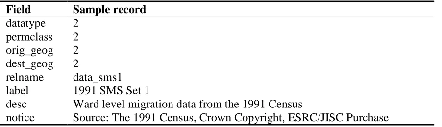
It can be seen in Table 2 that the first four values are numeric. It should be noted that the first value (datatype) forms the primary key (i.e. a unique identifier) for this table, whilst the next three are all – in SQL terms – foreign keys. This means that they can be used to look-up further information in other tables. The interaction data are being held in a table called ‘data_sms1’, and the ‘label’ and ‘desc’ fields give some basic description of what is in the data set. Finally, the ‘notice’ field is used to hold a copyright notice. It should be noted that this last field is not obeying the strict database rules of ‘normalisation’. It is likely that this exact notice will be used for more than one data set, and thus if it is held in full for each case, we will have data redundancy. The table should really store a foreign key, which is used to look up an entry in a separate table listing the known copyright notice types.

Table 2: Sample entries for fields in ‘meta_datasets’ for 1991 SMS Set 1

Field Sample record

datatype 2 permclass 2 orig_geog 2 dest_geog 2

relname data_sms1 label 1991 SMS Set 1

desc Ward level migration data from the 1991 Census

notice Source: The 1991 Census, Crown Copyright, ESRC/JISC Purchase

Table 3: Fields in ‘meta_tables’ and their uses

Field Use

datatype The datatype of the dataset in which this table can be found table_id A unique identifier for this table

title The title of this table

rowdef A text string listing the variables which define the rows of this table coldef A text string listing the variables which define the columns of this table map A keyword describing the mapping of data for this table in the data vectors

of the data set in which this table can be found (see text for description) rt_hint A ‘true-false’ toggle hinting whether row totals would be sensible for this

table

ct_hint A ‘true-false’ toggle hinting whether column totals would be sensible for this table

Table 4: Sample entries in ‘meta_tables’ for Tables 1 and 2 of the 1991 SMS Set 1

Field Sample record 1 Sample record 2

datatype 2 2

table_id 1 2

title All migrants: age (5 broad age groups) by sex

Wholly Moving Households and residents in Wholly Moving Households: counts

rowdef age1 count1

coldef sex1 wmhh1+res_in_wmhh1

map row row

rt_hint t f

ct_hint t f

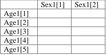
The first record has a simple table definition, consisting of a single sub-table component. This sub-table is 2-way crosstabulation using the variable ‘age1’ for rows, and the variable ‘sex1’ for columns. These (and all) variable labels are referenced to an additional metadata table, ‘meta_vars’. This metadata table is described fully below, but it is useful to understand at this point that it stores information about each variable including the number of categories for each variable. In the case of this example, the variable 'sex1’ has (unsurprisingly) 2 categories, whilst ‘age1’ is a variable giving a broad disaggregation of age with 5 categories. Thus, this record defines a table with five row categories and two column categories, as illustrated in Table 5.

Table 5: Basic layout of the table defined in Table 4, sample record 1.

Sex1[1] Sex1[2] Age1[1]

Age1[2] Age1[3] Age1[4] Age1[5]

patterns in order to maintain consistency with the published documentation. For this reason, the field ‘map’ is used in the metadata table ‘meta_tables’. This field uses a keyword to describe the field ordering pattern. There are three alternative keywords (‘row’, ‘col’ and ‘colskip’) covering all patterns in present use. If additional data sets introduce further patterns, a new keyword would need to be introduced, and suitable processing code added to WICID’s table layout and interpretation routines.

The second record in Table 4 defines a more complicated table. It can be seen that the ‘coldef’ field for this record refers to two variables – ‘wmhh1’ and ‘res_in_wmhh1’ – and that these are joined with a ‘+’ character. Again, details about the actual variables are held in the table ‘meta_vars’. This format indictates an overall table which is composed of two component sub-tables. The first sub-table is specified by the row variable ‘count1’ and the first column variable ‘wmhh1’, whilst the second is specified (again) by the row variable ‘count1’, and by the second column variable, ‘res_in_wmhh1’. The row variable is also an example of the use of a dummy variable – ‘count1’, which is simply a frequency count – to allow a univariate table to be described as a 2-way crosstabulation. This is because both column variables have a single category: they are univariate observations. Table 6 shows the basic layout of the table defined in the second record.

Table 6: Basic layout of the table defined in Table 4, sample record 2

wmhh1[1] res_in_wmhh1[1] count1[1]

a table to be defined as ‘age1,sex1’, then WICID would understand this to mean that rows should use the categories of sex1 iterated within each category of age1.

The final two fields in the ‘meta_tables’ metadata table are ‘rt_hint’ and ‘ct_hint’. These are Boolean fields which can optionally be used to draw an enhanced table. They hint to the system whether or not row and col (respectively) totals would be valid. In the examples in Table 4, these are both set to ‘t’ (i.e. true) for the age by sex table in record 1. This is because the totals of either of these variables (for a given case of the other variable) would be meaningful. On the other hand, both variables are set to ‘f’ in the second record, because neither row nor column totals would be meaningful – column totals would be a total of a single value, and therefore unnecessary, whilst a row total would be a total of two fields measuring different things.

As explained above, flow disaggregation tables are defined in terms of sub-table blocks, which are cross-tabulations of two or more variables. These variables are defined in the metadata table ‘meta_vars’. Table 7 describes the fields in this metadata table.

Table 7: Fields in ‘meta_vars’ and their uses

Field Use

var_id A unique identifier for this variable title The title of this variable

cats A count of the number of categories in this variable

labels_relname The name of a database table which holds the labels for each category index A Boolean toggle indicating whether or not this variable should be

included in an index of known variables

metadata table ‘meta_tables’. There are a number of cases in which some fundamental variable in the data is represented in alternative ways, for example the use of different groupings of age. Alternative classifications are all represented as separate variables in WICID, and thus there are several age variables defined in ‘meta_vars’ with the identifiers ‘age1’, ‘age2’ and so on. It should be noted that the numeric suffix in these names refers to alternative classifications rather than to categories within a generic ‘age’ variable.

that it would be confusing to include them in an index of all variables. The ‘index’ field allows such variables to be identified, by setting the value to ‘false’.

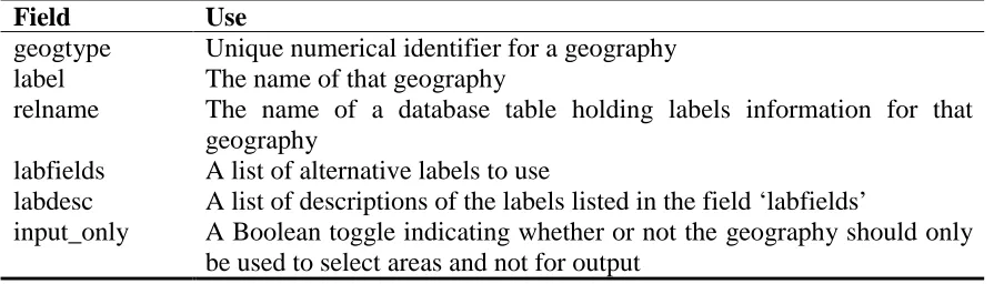
The metadata table ‘meta_vars’ holds data about all the variables by which data are classified with the important exception of geographical area. The geography data is held in two metadata tables, ‘meta_geog’ and a supporting table, ‘meta_geoglut’. Table 8 shows the structure of ‘meta_geog’. A record is held in ‘meta_geog’ for each geography that is used in the WICID system. A geography is any particular set of areas (e.g. wards, counties, parliamentary constituencies) that are used to subdivide1 the country.

Table 8: Fields in ‘meta_geog’ and their uses

Field Use

geogtype Unique numerical identifier for a geography label The name of that geography

relname The name of a database table holding labels information for that geography

labfields A list of alternative labels to use

labdesc A list of descriptions of the labels listed in the field ‘labfields’

input_only A Boolean toggle indicating whether or not the geography should only be used to select areas and not for output

relationships between geographies and dates are complex, and they are not currently well modelled in the WICID system. The reference to ‘1991’ in the label field in the example in Table 9 is – as far as the database is concerned – an arbitrary set of characters with no special meaning. It is currently up to the database administrator to make sure that data sets are defined in the metadata table ‘meta_datasets’ as having appropriate base geographies.

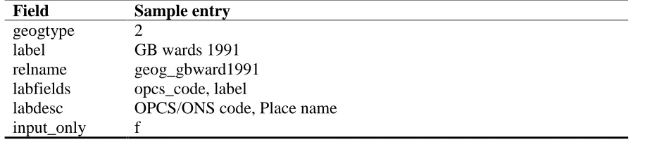
Table 9: Sample entry in ‘meta_geog’

Field Sample entry

geogtype 2

label GB wards 1991 relname geog_gbward1991 labfields opcs_code, label

labdesc OPCS/ONS code, Place name input_only f

The field ‘relname’ in ‘meta_geog’ refers to a database table holding a set of place identifiers for the geography. The present structure assumes that all geographies use a numeric sequence number as their primary identifier – all interaction data sets in WICID have origin and destination coded numerically. Attached to these sequence numbers can be any number of alternative identifiers, such as the OPCS/ONS ids (e.g. 08DAFA) familiar to most existing users of Census data, or place names (e.g. Aireborough). Different geographies will have different valid sets of identifiers, and therefore the fields ‘labfields’ and ‘labdesc’ are used to hold a list of fields within the database table defined by ‘relname’ and a list of matching text descriptions respectively.

1

The final field in ‘meta_geog’ is called ‘input_only’. This is not currently used by WICID, but intended to facilitate future use. Some geographies are meaningful to users, but cannot easily be used to output data. The main example of this is postal geography. By setting ‘input_only’ to ‘true’, it would be possible to identify geographies which could be used by the user to select a set of areas in another geography. Using the example of postal geography, a user may be able to type in a postcode, and generate output for the set of wards which best approximate that postcode area.

The example of the use of postal geography introduces the topic of translation from one geography to another. The ability to aggregate data to different geographies is one of the key facilities provided by WICID. In order to perform such aggregations, it is necessary to store metadata listing the relationships between different geographies. These metadata are held in the metadata table ‘meta_geoglut’, the fields of which are described in Table 10.

it can be seen that the first five wards all form part of both the first district and the first county.

Table 10: Fields in ‘meta_geoglut’ and their uses

Field Use

from_geogtype The geogtype (as listed in meta_geog) of a geography which can be aggregated to some other geography

to_geogtype The geogtype (as listed in meta_geog) of the geography to which the from_geogtype will be aggregated

lut_relname The name of a database table holding the look-up table which details the mapping needed for the aggregation

from_field The name of a field in the table mentioned in ‘lut_relname’ which lists identifiers of the geography specified by the ‘from_geogtype’

to_field The name of a field in the table mentioned in ‘lut_relname’ which lists identifiers of the geography specified by the ‘to_geogtype’

weight_field The name of a field in the table mentioned in ‘lut_relname’ gives a weight for each individual from-to-to mapping

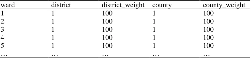
Table 11: Part of the database table lut_gbward1991

ward district district_weight county county_weight

1 1 100 1 100

2 1 100 1 100

3 1 100 1 100

4 1 100 1 100

5 1 100 1 100

… … … … …

giving a weight for each entry in the LUT. In Table 11, all weights are shown as being 100. Thus, for example, the first line in the table indicates that 100% of the count for ward 1 should be added to the total for the first district (along with 100% of the count for wards 2, 3, 4, 5 and so on). At present all aggregations use a consistent hierarchy of areas, such that all weights in all LUTs are set to 100. As all the weights are equal they can effectively be ignored, and these may be termed ‘unweighted LUTs’. The WICID system has been written with the expectation that at some stage it will be necessary to use mappings which cannot be achieved with unweighted LUTs. Instead, some fraction of the count for a ‘from’ area will be added to one ‘to’ area, with the remainder being added to a second ‘to’ area. An example of this would be the use of a post-1998 local authority geography, in which some wards have been split up and the components added to different new areas. If we wish to tabulate data that has 1991 base geographies at 1998 LA level, then we would need to use a weighted look-up table. This process is not ideal, and it would be preferable to use an alternative data set which has been modelled and re-estimated for the 1998 geography, but weighted LUTs allow a tabulation to be performed where no such data set exists.

is used internally, and is not revealed to the user. This internal id has certain properties: it is of a fixed length, and it is generated when a new user is created in the system using a seeded cryptographic function (md5) which should make the the value for any user difficult to predict. This ‘secret’ identifier is used as part of the WICID security system.

Table 12: Fields in ‘meta_users’ and their uses

Field Use

user_id Unique user id username User’s name password Password field

perms Interface permissions of user data_perms Data permissions of user

Table 13: Fields in ‘meta_dataperms’ and their uses

Field Use

permclass Unique identifier for permission class label Short label of permission type

desc Longer description of permission type

The final metadata table is ‘meta_usage’. This table is used to log all data extractions performed by WICID. The table fields are shown in Table 14. Each WICID query is split up internally into requests for data from different data sets, and then a series of 1 or more individual SQL queries are generated that extract the required data from that dataset. These individual queries are referred to as ‘chunks’. Whenever a data extraction occurs, the details of it are recorded in ‘meta_usage’. The field ‘username’ records the name of the user making the extraction, whilst the field ‘tstamp’ logs the precise date and time that the extraction was made. Within WICID, the time taken to carry out the extraction for a given data set (in one or more SQL chunk) is recorded. This value is logged in the field ‘time’. The final two fields record the dataset from which the data was extracted, and the number of chunks into which the query was split. The latter information is kept to assist the process of monitoring performance of the query building process.

Table 14: Fields in ‘meta_usage’ and their uses

Field Sample entry

username User’s name

tstamp Time and date that this entry was logged time Time taken in seconds to execute query datatype Datatype of dataset used in query

5 Using the Interface

In this section of the paper, the current version of the WICID interface is illustrated using a selection of screens or Webpages. Some of the features that appear on particular pages have not yet been implemented.

5.1 Login and the general user interface

The initial page to which potential users of WICID will be directed is the Login page (Figure 4) where users registered to extract data from the SMS and SWS will input their userids and passwords and where unregistered users will be able to type in a ‘guest’ userid and password to browse the system and access the sample of ‘blurred’ data. Once logged into WICID, the first page to appear will be a welcome page (Figure 5), with links to the general query interface, the library of popular data sets (and their associated queries) and pages of information about the interface and the data.

interface (WICID query) and the Current query. It is envisaged that this line will also contain a link to a page containing other census Web sites and a link that allows either a current query to be saved or an existing query to be restored.

The general query interface (Figure 6) is where the user can identify whether the query has been completed or not and whether data extraction can go ahead. Each data extraction query requires the selection of geographical areas (Geography) and tables or flows (Data). Both parts of the query must be prepared before any data can be extracted. The two parts may be completed in any order, can be revisited and adapted if required. Traffic light icons are used to indicate whether each section ‘Needs attention’ or is ‘Ready’. When each part has been prepared satisfactorily, the traffic light icon will be green and when both traffic lights are green, it becomes possible to proceed to the extraction phase.

5.2 Selection of geographical areas

Figure 4: WICID login screen

Figure 6: WICID general query interface

Figure 8: WICID area selection tools

Once the origins and destination areas or area lists have been selected, the remaining piece of information required to complete the Geography section is the choice of the type of flow required. Figure 10 illustrates the flow type selection page. Here, the user is confronted with a schematic table of possible flow types, and tick boxes with which to select flows between origins and destinations and within common areas, total outflows from all origins, total inflows to all destinations and/or total migration flows taking place in the system. WICID computes the number of counts associated with each of these options and indicates these values in the right hand column on the page. Once options have been selected, the values are highlighted. There is also a filter available to allow the option of selecting all flows, both between and within areas to fine tune the previous selections. An update button beneath the table will allow the flow types identified on the page to be selected.

5.3 Selection of variables

illustrates the table layout for SMS Set 2 Table 1: All migrants: age (5 broad age groups and sex).

5.4 Extraction and output

Figure 10: WICID flow type selection

Figure 12: WICID data set selection

Figure 14: WICID variable selection

Figure 16: WICID simple query

Clicking on the Output link on the query interface page takes the user to the output page which allows a variety of alternative layout and labelling options to be selected (Figure 18). Output can be generated in matrix form as an origin-destination pair list. Published table frameworks and bespoke layout options allowing users to design their own output will be implemented in due course. Format options allow output to be produced as an HTML table or in a comma separated (.csv) file. Delivery may be to the screen, to a file for downloading or as a file (generated from a batch run) for sending via email. A separate label selection page (Figure 19) allows the user to specify using tick boxes what form of origin and destination labels are required on the output. Once these output selections have been made, output may be previewed (Figure 20) before being being finally produced.

Figure 20: WICID output preview

6 2001 Census Interaction Data

WICID is being developed with a view to providing an interface to the origin-destination statistics produced from the 2001 Census. The Census Offices have proposed that the standard products will be SMS and the SWS for England and Wales plus Special Commuting Statistics (SCS) for Scotland - based on journeys to places of work and study. These data sets would contain the ‘flow’ elements equivalent to the 1991 SMS and SWS. It is proposed that some or all of the output for migrants by zone of origin and workers/commuters by zone of destination would be moved into the standard tables. This means that counts of out-migrants as well as in-migrants will be available for different zones. In preparation for the 2001 Census, the Census Offices have consulted on a wide range of issues relating to the origin-destination statistics and their proposed tabulations (ONS/GROS/NISRA, 1999; 2000). It is proposed that origin-destination products for 2001 will be based on data processed for 100% of census records and it is also assumed that a set of postcode-based Output Areas will be created for the whole of the UK for

Area Statistics.

Number Census (ONC) process which aims to add records to the database for missed

households and for missed individuals in otherwise enumerated households. As in previous censuses, the Census Offices intend to make a number of amendments to the data so as to prevent users of the data from making any deduction about a household or individual record. The method of statistical disclosure control has not yet been decided.

SMS Set 1 will include the flows between local authority areas, into local authority areas from outside the UK, into local authority areas when no usual residence one year ago was given or where origin is unknown. Throughout the tables, the term ‘sex’ used in 1991 is replaced by the term ‘gender’. The set of proposed tables for SMS 1 are likely to be as follows:

Table 1: Migrants by age and gender (40 variables);

Table 2: Migrants in households by family status and gender (18 variables); Table 3: Migrants by ethnic group and gender (14 variables);

Table 4: Migrants with or without limiting long term illness by gender (8

variables);

Table 5: Migrants aged 16 to 75 by economic position and gender (20 variables); Table 6: Moving groups of migrants in households (8 variables);

Table 7: Moving groups of migrants in households by tenure (16 variables); Table 8: Moving groups of migrants in households by gender and economic

position of head of group (80 variables);

Table 9: Moving groups of migrants in households by NS-SEC of head of group

Table 10: Migrants resident in Scotland/Wales/NI who know Gaelic/Welsh/Irish

family status and gender (18 variables).

SMS Set 2 in 2001 are due to contain the flows between wards or postcode sectors in Scotland. Four tables comprising Set 2 are proposed as follows:

Table 1: Migrants by age group and gender (22 variables); Table 2: Moving groups of migrants in households (4 variables); Table 3: Migrants by ethnic group and gender (4 variables); and

Table 4: Moving groups of migrants in households by NS-SEC of head of group

(24 variables).

As in 1991, it is proposed that there will be three sets of journey to work/study tables but unlike 1991, the three sets of tables will include interaction flows. SWS/SCS 1 will include flows between local authorities; SWS/SCS 2 will include flows between wards or postal sectors and SWS/SCS 3 will include flows between output areas. The proposed tables for SWS 1 are as follows:

Table 6: Workers by NS-SEC of head of group and gender (32 variables); and Table 7: Workers by ethnic group (7 variables).

Proposed tables for SWS 2 are as follows:

Table 1: Workers by broad age group (5 variables); Table 2: Workers by gender (2 variables);

Table 3: Workers by family status (7 variables);

Table 4: Workers by hours worked and gender (6 variables);

Table 5: Workers by method of travel to work/study (11 variables); and Table 6: Workers by NS-SEC (12 variables)

There is only one table proposed for SWS 3:

Table 1: Workers by method of travel to work/study (11 variables).

The tables proposed for the SCS 1 are as follows:

Table 1: Students and schoolchildren by age and gender (10 variables);

Table 2: Students and schoolchildren by family status and gender (18 variables);

and

For SCS 2, there are three tables proposed as follows:

Table 1: Students and schoolchildren by age group (5 variables); Table 2: Students and schoolchildren by gender (2 variables); and Table 3: Students and schoolchildren by family status (7 variables).

The proposed table for SCS 3 is as follows:

Table 1: Students and schoolchildren by method of travel to study.

It is envisaged that WICID will be able to provide the interface to these data in 2003 although some additional work will be necessary to construct the relevant pages and modify the software.

7 Conclusions

This paper has reviewed the data sets that will be accessed by WICID, has explained in detail the relationships between the software components of the information system and has illustrated the framework of metadata that underpins the system. The paper has also illustrated how the user will interact with the interface. Some progress has been made on the development of the WICID interface since the previous workshop. The project has now reached a point where access to the following data sets is a reality:

1991 SMS 2 Tables 1-12 (93 variables); and 1991 SWS C Tables 1-9 (274 variables).

By the end of the project, we intend to provide access to the following data sets:

1991 SMS 2 Tables 3-10 adjusted for suppression (89 variables);

1991 SMS 2 Table 3 adjusted for suppression, underenumeration and

mis-reporting (38 variables);

1981 SMS 2 Table 1 re-estimated for 1991 ward boundaries (2 variables); and 1981 SWS C Tables 1-5 re-estimated for 1991 ward boundaries (variables to be

determined).

Some data verification has been undertaken using the raw interaction flows extracted from the 1991 SMS. This has involved running equivalent queries with SMSTAB and with WICID and checking for consistency. In future, we intend to check unsuppressed flows for aggregate geographical areas (e.g regions) extracted from WICID with those available in the published 1991 Census reports.

the library of popular data sets and their associated queries; the save and restore queries facility;

the select by variable facility the analysis section;

the mapping section; the Help system; and

References

Ballard, B. and Norris, P. (1983) User needs – an overview, Chapter 3 in Rhind, D. (ed) A

Census User’s Handbook, Methuen London: 89-113.

Boyle, P. (1995) Modelling population movement into the Scottish highlands and islands from the remainder of Britain, 1990-1991, Scottish Geographical Magazine, 111(1).

Boyle, P.J., Flowerdew, R. and Shen, J. (1998) Modelling inter-ward migration in Hereford and Worcester: the importance of housing growth and tenure, Regional

Studies, 32(2): 113-32.

Champion, A.G. (1994) Population change and migration in Briatin since 1981: evidence for continuing deconcentration, Environment and Planning A, 10: 1501-20.

Champion, A.G. and Atkins, D.J. (1996) The counterurbanisation cascade: an analysis of the 1991 Census Special Migration Statistics for Great Britain, Seminar Paper 66, Department of Geography, University of Newcastle upon Tyne.

Cole, K. (1995) Why are the Special Workplace and Migration Statistics Special? MIDAS

Newsletter 3, MIDAS, Manchester.

Cole, K. and Squires, S. (1987) The Special Migration Statistics from the 1981 Census: the data and their implications, Paper presented at the LAMSAC workshop, County Hall, London.

Duke-Williams, O. (1997) A Guide to Using the 1991 Special Migration and Workplace Statistics on MIDAS, Working Paper, School of Geography, University of Leeds, Leeds.

Flowerdew, R. and Boyle, P. (1992) Migration trends for the West Midlands: suburbanisation, counterurbanisation or rural depopulation?, Chapter 9 in Stillwell, J., Rees, P. and Boden, P. (eds.) Migration Processes and Patterns

Volume 2: Population Redistribution in the United Kingdom, Belhaven Press,

London: 144-161.

Flowerdew, R.; Boyle, P. J. (1995) Migration models incorporating interdependence of movers, Environment and Planning A, 27(9): 1,493-502.

Frost, M., Linneker, B. and Spence, N. (1996) The spatial externalities of car-based wortravel emissions in Greater London, 1981 and 1991, Transport Policy, 3, 187-200.

Frost, M., Linneker, B. J. and Spence, N. (1997) The energy consumption implications of changing worktravel in London, Birmingham and Manchester: 1981 and 1991,

Transportation Research A, 31(1): 1-19.

Frost, M., Linneker, B. and Spence, N. (1998) Excess or wasteful commuting in a selection of British cities, Transportation Research A, 32, 529-538.

Forster, E. (1998) Exploring internal migration in Scotland: getting underneath the patterns and unpacking the processes, Poster Paper, Popfest Online 1(1).

OPCS/GRO(S) (1993a) 1991 Census User Guide 35 Special Migration Statistics:

Prospectus, OPCS and GRO(S).

OPCS/GRO(S) (1993b) 1991 Census User Guide 36 Special Workplace Statistics:

Prospectus, OPCS and GRO(S).

OPCS/GRO(S) (1993c) 1991 Census User Guide 51 Special Migration Statistics: Cell

Numbering Layouts, OPCS and GRO(S).

OPCS/GRO(S) (1993d) 1991 Census User Guide 52 Special Workplace Statistics: Cell

Numbering Layouts, OPCS and GRO(S).

ONS/GROS/NISRA (1999) 2001 Census: Output: A Discussion Paper.

Origin-Destination Output (Workplace/commuting and migration), Unpublished Paper.

ONS/GROS/NISRA (2000) Origin-Destination Statistics A Discussion Paper, Consultations, June 2000.

Rees, P.H. and Duke-Williams, O. (1994) The Special Migration Statistics: a vital resource for research into British migration, Working Paper 94/20, School of Geography, University of Leeds, Leeds.

Rees, P.H. and Duke-Williams, O. (1995) The story of the British special migration statistics, Scottish Geographical Magazine, 11: 13-26.

Rees, P.H. and Duke-Williams, O. (1997) Methods for estimating missing data on migrants in the 1991 British Census, International Journal of Population

Geography, 3: 323-368.

Simpson, S. and Middleton, E. (1999) Undercount of migration in the UK 1991 Census and its impact on counterurbanisation and population projections, International

Spence, N. A. and Frost, M. (1995) Worktravel responses to changing workplaces and changing residences, in Brochie, J. et al (eds) Cities in Competition: Productive

and Sustainable Cities for the 21st Century, Longman: Melbourne, 359-381.

Turton, I. and Openshaw, S. (1998) Human Systems Modelling: Results of the HPC

Initiative at Leeds, Centre for Computational Geography, School of Geography,

University of Leeds.