Partial quadratic eigenvalue assignment in vibrating systems using
acceleration and velocity feedback
Jiafan Zhanga, Huajiang Ouyangb,*, Yonglin Zhanga, Jianping Yea
aSchool of Mechanical Engineering, Wuhan Polytechnic University, Wuhan, 430023,
People’s Republic of China
bSchool of Engineering, University of Liverpool, Liverpool L69 3GH, UK
Partial quadratic eigenvalue assignment in vibrating systems using
acceleration and velocity feedback
The partial quadratic eigenvalue assignment problem (PQEVAP) is to shift a few undesired eigenvalues of a damped vibrating system to suitably chosen locations, while leaving the remaining eigenvalues and corresponding eigenvectors unchanged. In this paper, an algorithm for solving PQEVAPs and the minimum norm PQEVAP (MNPQEVAP) using acceleration and velocity feedback is proposed. It is shown that solving the PQEVAP here is transformed into solving an eigenvalue assignment of a linear system of a much lower order. Furthermore, the MNPQEVAP here can be efficiently solved by a gradient-based unconstrained optimization method with the derived gradient formula. This algorithm works directly on the second-order system model, and requires the knowledge of only the open-loop eigenvalues to be replaced and their corresponding eigenvectors. Lastly, through two numerical examples, the results of solving the MNPQEVAP under two different combined feedback signals, velocity and displacement signals, and acceleration and velocity signals, are compared from two points of view, i.e. the F-norms of their feedback matrices and the active control energy required from the actuators.
Keywords:vibrating system; partial quadratic eigenvalue assignment; acceleration and velocity feedback; minimum norm
65F18; 70J50; 93B52
1. Introduction
(1) where , and are all real constant n×n matrices, and are, respectively, mass, damping, and stiffness matrices. and are real n-vectors, and represent, respectively, the system responses and external forces, and nis an integer and denotes the number of degrees of freedom (d.o.f.) of the system.
The dynamical behavior of a vibrating system modeled by (1) is governed by the eigenvalues and eigenvectors of the corresponding quadratic matrix pencil :
(2) where scalar and the associated nonzero vector and , which satisfy
, ( ) (3)
are, respectively, the eigenvalue and the right and left eigenvectors of the quadratic matrix pencil . The eigenvalues contain natural frequencies and eigenvectors are mode shapes of in vibration theory. Together, or is called a right or lefteigenpair of (1). It is known that has 2nfinite eigenvalues over the complex field, provided that the mass matrix is non-singular. Additionally, system (1) and the quadratic matrix pencil are known as an open-loop system and an open-loop quadratic matrix pencil, respectively.
which was then generalized to the multi-input case by Datta and Sarkissian in [2] and Ram and Elhay in [3]. Because of its significance in the active control of a large or complicated vibrating system, and the challenges in its theory and numerical approaches, considerable efforts have been made to solve PQEVAP, both theoretically and computationally, especially working directly on second-order dynamic system models. A partial list of published works includes those reported in [4-11]. It should be noted that another important, related and more complex research work, that is, partial quadratic eigenstructure assignment problem, is not studied in this paper.
To implement a multi-input state feedback control strategy, a control force of the form is applied to the structure. Here B is a given real n×m control matrix ( ), and for convenience, is assumed to be of full column rank; and is a real time-dependent m-vector. Because the system is of second-order, active control using velocity and displacement feedback or acceleration and velocity feedback can be used to assign the eigenvalues, where takes the following special forms, respectively:
, (4)
. (5)
where F1 and G1, and F2and G2 are unknown, constant real n×m matrices, called the feedback gain matrices. From (1) and (4) or (1) and (5), the corresponding closed-loop systems are as follows:
, (6)
. (7)
They have the corresponding closed-loop quadratic matrix pencils as follows:
. (9) Solving the PQEVAP is to find feedback matrices in (4) or (5) such that the quadratic pencil (8) or (9) has the specified eigenvalues. It should be noted that, using a variable transformation 𝜆 = 1 𝜇 in (8) or (9), 𝐅1, 𝐆1or 𝐅2, 𝐆2 solving the PQEVAP using
velocity and displacement, or acceleration and velocity feedback control can be transformed to solving the PQEVAP with reciprocal eigenvalues 𝜇 under acceleration
and velocity, or velocity and displacement feedback control. Thus, the corresponding closed-loop quadratic matrix pencils become, respectively,
, (10)
. (11)
It is required for and to be non-singular so that the closed-loop
eigenvalues of (8) or (10) are finite and non-zeros; so is for and of (9) or
(11). Additionally, eqs. (9) and (10) clearly show that the affected system matrices are different for these two solution approaches to PQEVAP using acceleration and velocity feedback control.
reducing noise amplification [12]. High feedback gains or high condition numbers often lead to high sensitivity of the closed-loop eigenvalues.
Another observation is that all these approaches use combined velocity and displacement feedback control to solve PQEVAP. From the open literature, works on PQEVAP using acceleration and velocity feedback are rare. Using these feedback signals is even more interesting because of the frequent use of accelerometers in practice. In [13], Datta et al. once mentioned state feedback control using acceleration and velocity to assign partial quadratic eigenstructure. Recently, Abdelaziz [14] used velocity-plus-acceleration feedback to assign the full eigenstructure of second-order systems, and extended the established results from first-order systems to second-order systems. The same author also considered the robust pole assignment problem using combined velocity and acceleration feedback for second-order linear systems in [15].
In addition to the eigenvalue assignment methods mentioned above, which can be classified as the model-based approach, it is worthwhile to point out that a new approach to eigenvalues assignment in structural vibration systems was introduced by Ram and Mottershead [16], and extended by them and their colleagues [17-20] based on measured receptances and without the need to know or evaluate system matrices M,C andK. A recent paper by Ram and Mottershead [21] developed a new theory for active vibration control by pole placement using the receptance method. The formulation presented allowed for partial pole placement by multiple-input- multiple-output control using experimentally measured receptances, and it was demonstrated that the redundancy offered by multiple-input control may be used to assign not only the eigenvalues but also the eigenvectors of the system.
the active control energy required from the actuators under two control strategies, i.e., velocity and displacement feedback, acceleration and velocity feedback, is compared for the same numerical examples. These results give some insight into feedback control in solving PQEVAP in terms of the magnitude of the feedback gain matrices and the amount of actuation energy. In Section 2, some notations, definitions and assumptions are presented, which will be used throughout this paper. In Section 3, the theory on the solvability of the PQEVAP is analysed and the parameterized solutions to the PQEVAP are derived. The numerical approaches for solving the MNPQEVAP are presented in Section 4, and numerical results are given in Section 5 and analysed from the active control energy point of view. Finally, some concluding remarks are given in Section 6.
2. Notation and assumptions
To avoid complex arithmetic in this paper, the eigenpairs of the original structure (i.e. the open-loop system) and the corresponding actively controlled structure (i.e. the closed-loop system) are described using real representations [22, 23]. Without loss of generality, assume that the p eigenpairs of the original structure have the following forms:
, , and
.
The real representations of and are defined in the following forms:
. (13)
Similarly, let the real representation of the p prescribed partial eigenvalues of the controlled structure be
(14)
and the real representation of their corresponding right eigenvectors and left
eigenvectors be and , respectively, which are to be determined. Here the newly assigned eigenvalues containscomplex conjugate pairs, which is not necessarily equal tol. Also, let the remaining 2n−p eigenpairs of the original structure be denoted
by , and let the real representation of and be and
, respectively.
The p eigenpairs of the original structure with the corresponding true (complex-valued) eigenvalue matrices
and true (complex-valued) eigenvector matrices
, satisfy a system of algebraic equations as follows:
. (15)
In what follows, it is shown that the real representations (12) and (13) of also satisfy a system of algebraic equations like (15). Indeed, let
, (16)
, . (17) Substituting (17) into (15) and considering the fact that is non-singular and , one gets the system of algebraic equations that and should satisfy as follows:
. (18)
Similar algebraic equations also hold for and , that is
(19) and hold for the eigenpairs of the closed-loop system. In addition, it is known that, as indicated in [22], the p eigenvalues is precisely the spectrum of its real representation matrix , which is denoted by . Similarly, the eigenvalues set
and be denoted by and .
With the notation and analysis above, the PQEVAP using acceleration and velocity feedback can be stated as: given and satisfying (16), and , one is to find F2 andG2 such that
, (20)
, (21)
for somen×preal matrix .
Throughout the paper, the following assumptions stand:
(A1) and are symmetric; M is positive definite ( ), is non-singular,and control matrixBis of full column rank;
(A2) (an empty set), ,
(A3) and for ;
(A4) The original open-loop system is partially controllable for the eigenvalues
; that is, .
It should be noted that, in assumption (A1), stiffness matrixKbeing non-singular is required. The same requirement can be found in [1, 7, 8]. However, the algorithm in [11] does not require thatK is non-singular based on a different parameter expressions forF1andG1.
3. Parametric solutions to the PQEVAP for feedback matrices F2and G2
Firstly, two orthogonal equalities which are of critical importance in the following deduction are presented.
Let
.
It follows from (18) and (19) that , which implies , since matrices
and do not have common eigenvalues, i.e. . Thus the
following orthogonality relation is obtained
. (22)
Similarly, one can get another orthogonality relation
, (23)
Using (22), one has the following lemma concerning a necessary condition on the solvability of the PQEVAP.
Lemma 3.1. If there existF2andG2satisfying (21), and the eigenvalue matrix is non-singular, then they have the following forms
, (24)
, (25)
where is arbitrary.
Proof
Combining (19) and (21) leads to
, which implies
, (26)
sinceB is of full column rank and eigenvalue matrix is non-singular. On the other hand, from (22) it follows that
, (27)
since
.
Here N(·) and R (·) denote the null space and range of a matrix, respectively. Thus, it follows from (26) and (27) that there exists a matrix such that
,
Remark 3.1. In lemma 3.1 of [11], the authors gave the feedback matrices
and based on the displacement and velocity
feedback. Again, it is worthwhile to point out that the parametric expressions (24) and (25) for solutions F2and G2 given in this paper turn out to be in the same forms those for and reported in [1, 7, 8, 9], but the latter are associated with and expressed by the corresponding complex eigenvalues and eigenvectors and obtained under the displacement and velocity feedback strategy. It should be pointed out that in the approach presented in this paper and that in [11], the constructions of the feedback matrices do not involve complex arithmetic.
The following theorem gives a necessary and sufficient condition on the solvability of the PQEVAP withF2andG2, which presents a different formula from theorem 3.1 in [11].
Theorem 3.1. The PQEVAP is solvable with being of full column rank if
and only if there exists a matrix and a non-singular matrix such that
. (28)
And if (28) holds, the solutions to the PQEVAP are given by (24) and (25).
Proof
Necessity: Note that if there exist F2 and G2 such that (20) and (21) hold for a
matrix making have a full column rank, then from (23) and (27), one
knows that there must exist a non-singular matrix such that
Expanding the two sides of (29), one immediately obtains
, (30)
since is non-singular. Another equality obtained is
. (31)
Then substituting (24) and (30) into (31), one gets
, (32)
sinceMis non-singular.
On the other hand, substituting (24), (25), (30) and (32) into (20) gives
,
where the second equality uses (30), the third equality uses (24) and (25), and the fourth
equality uses (32). Substituting into of the
last equality, and then post-multiplying the resultant equality by , one gets
.(33)
Additionally, multiplying (32) byMand on the left and right, respectively, gives
. (34)
Then Equation (33), together with (34), gives rise to
. (35)
, (36)
and matrix
is of full column rank, it follows immediately by comparing (35) with (36) that
, (37a)
or
. (37b)
Because and are invertible in view of the assumptions (A1), (A2), (A3), and
, it follows from (37b) that or
. It is observed from the last formula that (28) holds, which completes the proof of necessity.
Conversely, if there exist a matrix and a non-singular matrix
such that (28) holds, itcan easily be verified that is of full column rank by
letting , and (20) and (21) hold, whereF2andG2are given by (24) and (25), respectively. Thus, the proof is completed. □
Theorem 3.1 above shows that the PQEVAP using the acceleration and velocity
feedback is solvable with being of full column rank if and only if (28) is
As is well known, for a first-order linear system of the state-space form: . Let be an appropriate scalar set in the complex plane. The eigenvalue assignment problem of the first-order system is that, given the controllable pair (A,E), determining the state feedback matrixFof the appropriate dimensions such that the eigenvalues of the closed-loop state matrix A + EF are at desired locations in
. Now taking the transpose operation of (26) gives
, (38)
which means that the eigenvalues of matrix are the same as those of matrix . Here, matrix is similar to the closed-loop state matrixA +
EF of the first-order linear system above; the eigenvalues of matrix are eigenvalues of the closed-loop first-order model. So, solving the PQEVAP according to Theorem 3.1 is just that, given a first-order linear system , one has to find a
feedback matrix , such that the closed-loop eigenvalues are the eigenvalues of matrix . The Schur method is an efficient method for this problem [24].
It is well known that this linear eigenvalue assignment problem is solvable if and only if is controllable. Again, similarly as in theorem 3.2 in [11], it can be proved that the partial controllability of the original open-loop system (1) for eigenvalues is equivalent to the controllability of . Details of the proof are omitted here.
prescribed partial eigenvalues are finite and nonzero, it can be guaranteed that
the resultant closed-loop mass matrix in this paper is non-singular.
4. Solving MNPQEVAP for feedback matrices F2and G2
As mentioned above, it is suitable to use the Schur method to the problem (28) to obtain matrix , and then the solution F2 and G2 to the PQEVAP is obtained by (24) and (25). However, this has not involved minimizing the norms of the feedback matrices, which is denoted as the MNPQEVAP and presented below.
The MNPQEVAP is to minimize the norms of the feedback matricesF2andG2. Let
, (39)
where Q1 is the matrix made up from the first p columns of the orthogonal matrix , and is a non-singular upper triangular matrix. Then using (24) and (25), the objective function to be minimized in the MNPQEVAP becomes
.(40)
On the other hand, feedback matricesF2 and G2 also need to satisfy the following algebraic equation:
, (41a)
. (41b)
Let
, (42)
then it follows that , which implies that D is symmetric, and D can be proved, similarly as in [11], to be non-singular. Using (29), (42) can be rewritten as
. (43)
Substituting (43) into (41b) gives
, (44)
where
, (45a)
. (45b)
Additionally, in term of (45a), (45b), and , (28) can be rewritten as
.
Pre-multiplying both sides of the last equality by , and rearranging, gives
From Sylvester equation (46), one gets solution in term of , showing via vec operator which vectorizes a matrix by stacking its columns, as follows:
. (47)
Here denotes the Kronecker product. It should be noted that Sylvester equation (46) has a unique solution, because matrices and do not have common eigenvalues [25]. Now, using (45b), the objective functionfdefined in (38) can be rewritten as
, (48) which, together with (47), shows thatfis a function of .
After some manipulations, one can obtain the gradient offwith respect to as
, (49)
whereWsatisfies the Sylvester equation below
, (50)
with .
The solution of Sylvester equation (50) is represented by
. (51)
So the unconstrained optimization problem (40) or (48) can be solved by any gradient-based methods, such as ‘BFGS’, trust-region Newton’ method, etc. As indicated in [11], this kind of optimization problems may have many local minima, thus by solving the optimization problem repeatedly with different random initial values; one is able to find the feedback matrices in the case when the cost function has a very low value.
Algorithm 4.1:
Input: , , , , , and .
Output:F2andG2.
(1) Compute the ‘economy size’ QR decomposition
as in (39).
(2) Choose an initial matrix randomly, and then solve the optimization problem (48) by using a gradient-based method via (47), (51), and (49); find such
that .
(3) Solve Sylvester equation (46) with for , and then compute .
(4) ComputeF2andG2by (24) and (25).
5. Numerical examples
In this section, two numerical results for solving the MNPQEVAP using the algorithm 4.1 above and the algorithm in [11] are presented. The resultant feedback matrices, which are obtained using the same optimization method for the same examples and assignment requirements from the same initial matrix , are explored to compute the energy required from the actuators under two control strategies. Based on the energy (as an indicator of relative merits) defined by Soong [26], the actuation energy of the two control strategies are presented as follows:
, (53) which are squares of the combined active control forces during a time period [0,T].
The examples are computed using MATLAB 7.11. MATLAB function fminunc is used to solve the optimization problem in Step 2 of the algorithm with the gradient given by (49), based on the quasi-Newton ‘BFGS’ method.
Example 5.1(P 5.2 in [10]). MatricesM,C,K, andBare as follows:
, , .
The open-loop eigenvalues are: . This is an undamped
vibrating system. In this example, two partial eigenvalue assignment schemes are considered: (1) two eigenvalues are reassigned to , which is also the assignment of P 5.2 in [10]. This changes the two oscillatory frequency components into non-oscillatory decaying ones. (2) two eigenvalues are reassigned to , which changes the frequency and adds damping to the two frequency components.
Case (1): The resultant velocity and displacement feedback matrices and their F -norms are as follows:
, ,
TheF-norms ofF1andG1here are comparable with those of the pure MNPQEVAP, which are 19.36 and 70.89 in [10]. The resultant acceleration and velocity feedback matrices and theirF-norms are as follows:
, ,
, .
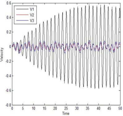
Now a new harmonic excitation is applied to the second d.o.f. This driving frequency is close to the third undamped natural frequency of the open-loop system. The time-domain responses of the open-loop system and two closed-loop systems with gains above are shown in Fig. 1. As the active control removes the undesirable undamped natural frequency value 3.6039 of the open-loop system, the original resonant response is suppressed significantly; and the steady-state response magnitude of the controlled system using the acceleration and velocity feedback is smaller than that of the controlled system using the velocity and displacement feedback, as shown in Fig. 1. Additionally, one has
, ,
Figure. 1. The velocity time history of the second d.o.f. of Example 5.1 Case (1): V1— the open-loop system; V2—the controlled system with the acceleration and velocity feedback; V3—the controlled system with the velocity and displacement feedback.
Case (2): The resultant velocity and displacement feedback matrices and their F -norms are as follows:
, ,
, .
The resultant acceleration and velocity feedback matrices and their F-norms are as follows:
, .
Applying the same excitation force in this case as in case (1), the time-domain responses of each system are shown in Fig. 2. The steady-state response magnitude of the controlled system using the acceleration and velocity feedback is nearly the same as that of the controlled system using the velocity and displacement feedback, as shown in Fig. 2. Additionally, one has
, ,
which again indicates similar amounts of energy consumption.
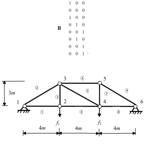
Example 5.2. A plane truss structure with 9 bars is shown in Fig. 3. Its material
parameters are: elastic modulus E=2.1e11Pa, mass density ρ=7860㎏/m3, cross sectional area of each bar A=2.5e-3m2. The plane truss is excited vertically by
N and to nodes 2 and 4, respectively.
These driving frequencies are close to the first and the second undamped natural frequencies of the truss structure, respectively. The damping matrix is taken asC=
1.0e-5*K+1.0e-4*M. This truss has open-loop eigenvalues: , ,
, , , , ,
. The undesirable first and second pairs of eigenvalues are reassigned to and . The other unassigned eigenpairs are kept unchanged. The control matrixBis
.
1 2 4
3 5 6 ② ① ③ ④ ⑤ ⑥ ⑦ ⑧ ⑨
4m 4m 4m
3m
f2
f1
The resultant velocity and displacement feedback matrices and theirF-norms are as follows:
, ,
, .
The resultant acceleration and velocity feedback matrices and their F-norms are as follows:
, ,
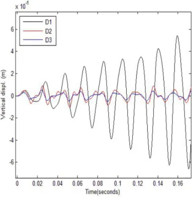
The time-domain responses of the original structure and two controlled structures with gains above are shown in Fig. 4. The steady-state response magnitude of the controlled structure using the acceleration and velocity feedback is slightly larger than that of using the velocity and displacement feedback. Additionally, one has here
, ,
which indicates that one needs slightly larger amount of energy to achieve the partial eigenvalues assignments in this example using the acceleration and velocity feedback, than that when using the velocity and displacement feedback.
Figure 4. The vertical displacement time history of the plane truss at node 4 of Example 5.2 : D1—the original structure; D2—the controlled structure with the acceleration and velocity feedback; D3—the controlled structure with the velocity and displacement feedback.
6. Conclusions
Partial quadratic eigenvalue assignment and associated minimum norm optimisation (PQEVAP and MNPQEVAP) are carried out using acceleration and velocity feedback in this paper. The algorithm proposed has some attractive practical features as in [11, 10, 7, 8, 9], which makes it suitable in dealing with large-scale practical structures. It is found in numerical examples that the PQEVAP and MNPQEVAP using acceleration and velocity feedback normally can be solved with similar amounts of actuation energy to those of velocity and displacement feedback. Both control strategies are shown to be capable of suppressing vibration.
Acknowledgements
The authors would like to thank the referees for their valuable comments. The work is carried out during the 6-month visit to the University of Liverpool by the first author who is sponsored by the China Scholarship Council and Hubei Education Authority.
References
[1] Datta BN, Elhay S, Ram YM. Orthogonality and partial pole assignment for the symmetric definite quadratic pencil. Linear Algebr. Appl. 1997; 257: 29–48.
[2] Datta BN, Sarkissian DR. Multi-input partial eigenvalue assignment for the symmetric quadratic pencil. The American Control Conference; 1999 June 2-4; San Diego, California, USA.
[3] Ram YM, Elhay S. Pole Assignment in Vibratory Systems by Multi-Input Control. J. Sound Vib. 2000; 230: 309–321.
[5] Chu EK. Pole assignment for second-order systems. Mech. Syst. Signal Pr. 2002; 16: 39–59.
[6] Datta BN. Finite element model updating and partial eigenvalue assignment in structural dynamics: recent developments on computational methods. 10th International Conference on Mathematical Modelling and Analysis and 2nd International Conference on Computational Methods in Applied Mathematics; 2005 June 1-5; Trakai, Lithuania. [7] Xu SF, Qian J. Orthogonal basis selection method for robust partial eigenvalue assignment problem in second-order control systems. J. Sound Vib. 2008; 317: 1–19. [8] Qian J, Xu SF. Robust partial eigenvalue assignment problem for the second-order system. J. Sound Vib. 2005; 282: 937–948.
[9] Brahma S, Datta BN. An optimization approach for minimum norm and robust partial quadratic eigenvalue assignment problems for vibrating structures. J. Sound Vib. 2009; 324: 471–489.
[10] Bai ZJ, Datta BN, Wang JW. Robust and minimum norm partial quadratic eigenvalue assignment in vibrating systems: a new optimization approach. Mech. Syst. Signal Pr. 2010; 24: 766–783.
[11] Cai YF, Qian J, Xu SF. The formulation and numerical method for partial quadratic eigenvalue assignment problems. Numer. Linear Algebr. 2011;184: 637–652.
[12] Varga A. Robust pole assignment via Sylvester equation based state feedback parameterization. The 2000 IEEE International Symposium on Computer-Aided Control System Design; 2000 September 25-27; Anchorage, Alaska, USA.
[13] Datta BN, Elhay S, Ram YM, Sarkissian DR. Partial eigenstructure assignment for the quadratic pencil. J. Sound Vib. 2000; 230: 101–110.
[15] Abdelaziz THS. Robust pole placement for second-order linear systems using velocity-plus-acceleration feedback. IET Control Theory & Appl. 2013; 7: 1843–1856. [16] Ram YM, Mottershead JE. Receptance method in active vibration control. AIAA Journal. 2007; 45: 562–567.
[17] Mottershead JE, Tehrani MG, James S, Ram YM. Active vibration suppression by pole-zero placement using measured receptances. J. Sound Vib. 2008; 311: 1391–1408. [18] Ouyang H. Pole assignment of friction-induced vibration for stabilisation through state-feedback control. J. Sound Vib. 2010; 329: 1985–1991.
[19] Tehrani MG, Mottershead JE, Shenton AT, Ram YM. Robust pole placement in structures by the method of receptances. Mech. Syst. Signal Pr. 2011; 25: 112–122. [20] Tehrani MG, Ouyang H. Receptance-based partial pole assignment for asymmetric systems using state-feedback. Shock Vib. 2012; 19: 1135-1142.
[21] Ram YM, Mottershead JE. Multiple-input active vibration control by partial pole placement using the method of receptances. Mech. Syst. Signal Pr. 2013; 40: 727–735.
[22]Chu MT, Kuo YC, Lin WW. On inverse quadratic eigenvalue problems with
partially prescribed eigenstructure. SIAM J. Matrix Anal. Appl. 2004; 25:
995–1020.
[23] Chu MT, Xu SF. Spectral decomposition of real symmetric quadratic λ-matrices
and its applications. Math. Comput. 2009; 78: 293–313.
[24] Varga A. A Schur method for pole assignment. IEEE Trans. Auto. Control. 1981; 26: 517–519.
[25] Datta BN. Numerical methods for linear control systems design and analysis. Boston: Elsevier Academic Press; 2003.
Figure 1. The velocity time history of the second d.o.f. of Example 5.1 Case (1): V1— the open-loop system; V2—the controlled system with the acceleration and velocity feedback; V3—the controlled system with the velocity and displacement feedback. Figure 2. The velocity time history of the second d.o.f. of Example 5.1 Case (2): V1— the open-loop system; V2—the controlled system with the acceleration and velocity feedback; V3—the controlled system with the velocity and displacement feedback. Figure 3. A plane truss with 9 bars.