SPH SPH
JWDD006-FM JWDD006-Larose November 23, 2005 14:49 Char Count= 0
DATA MINING
METHODS AND
MODELS
DANIEL T. LAROSE
Department of Mathematical Sciences Central Connecticut State UniversityA JOHN WILEY & SONS, INC PUBLICATION
DATA MINING
METHODS AND
MODELS
SPH SPH
JWDD006-FM JWDD006-Larose November 23, 2005 14:49 Char Count= 0
DATA MINING
METHODS AND
MODELS
DANIEL T. LAROSE
Department of Mathematical Sciences Central Connecticut State UniversityA JOHN WILEY & SONS, INC PUBLICATION
SPH SPH
JWDD006-FM JWDD006-Larose November 23, 2005 14:49 Char Count= 0
CopyrightC 2006 by John Wiley & Sons, Inc. All rights reserved.
Published by John Wiley & Sons, Inc., Hoboken, New Jersey. Published simultaneously in Canada.
No part of this publication may be reproduced, stored in a retrieval system, or transmitted in any form or by any means, electronic, mechanical, photocopying, recording, scanning, or otherwise, except as permitted under Section 107 or 108 of the 1976 United States Copyright Act, without either the prior written permission of the Publisher, or authorization through payment of the appropriate per-copy fee to the Copyright Clearance Center, Inc., 222 Rosewood Drive, Danvers, MA 01923, 978-750-8400, fax 978-646-8600, or on the web at www.copyright.com. Requests to the Publisher for permission should be addressed to the Permissions Department, John Wiley & Sons, Inc., 111 River Street, Hoboken, NJ 07030, (201) 748–6011, fax (201) 748–6008 or online at http://www.wiley.com/go/permission.
Limit of Liability/Disclaimer of Warranty: While the publisher and author have used their best efforts in preparing this book, they make no representations or warranties with respect to the accuracy or completeness of the contents of this book and specifically disclaim any implied warranties of merchantability or fitness for a particular purpose. No warranty may be created or extended by sales representatives or written sales materials. The advice and strategies contained herein may not be suitable for your situation. You should consult with a professional where appropriate. Neither the publisher nor author shall be liable for any loss of profit or any other commercial damages, including but not limited to special, incidental, consequential, or other damages.
For general information on our other products and services please contact our Customer Care Department within the U.S. at 877-762-2974, outside the U.S. at 317-572-3993 or fax 317-572-4002.
Wiley also publishes its books in a variety of electronic formats. Some content that appears in print, however, may not be available in electronic format. For more information about Wiley products, visit our web site at www.wiley.com
Library of Congress Cataloging-in-Publication Data:
Larose, Daniel T.
Data mining methods and models / Daniel T. Larose. p. cm.
Includes bibliographical references. ISBN-13 978-0-471-66656-1 ISBN-10 0-471-66656-4 (cloth) 1. Data mining. I. Title. QA76.9.D343L378 2005 005.74–dc22
2005010801
Printed in the United States of America
10 9 8 7 6 5 4 3 2 1
DEDICATION
To those who have gone before,
including my parents, Ernest Larose (1920–1981)
and Irene Larose (1924–2005),
and my daughter, Ellyriane Soleil Larose (1997–1997);
For those who come after,
including my daughters, Chantal Danielle Larose (1988)
and Ravel Renaissance Larose (1999),
and my son, Tristan Spring Larose (1999).
SPH SPH
JWDD006-FM JWDD006-Larose November 23, 2005 14:49 Char Count= 0
CONTENTS
PREFACE xi
1 DIMENSION REDUCTION METHODS 1
Need for Dimension Reduction in Data Mining 1
Principal Components Analysis 2
Applying Principal Components Analysis to theHousesData Set 5
How Many Components Should We Extract? 9
Profiling the Principal Components 13
Communalities 15
Validation of the Principal Components 17
Factor Analysis 18
Applying Factor Analysis to theAdultData Set 18
Factor Rotation 20
User-Defined Composites 23
Example of a User-Defined Composite 24
Summary 25
References 28
Exercises 28
2 REGRESSION MODELING 33
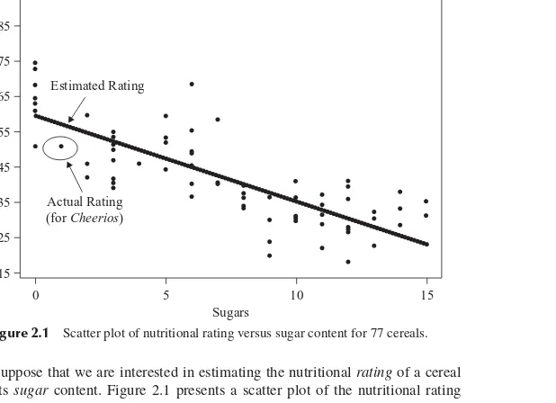
Example of Simple Linear Regression 34
Least-Squares Estimates 36
Coefficient of Determination 39
Standard Error of the Estimate 43
Correlation Coefficient 45
ANOVA Table 46
Outliers, High Leverage Points, and Influential Observations 48
Regression Model 55
Inference in Regression 57
t-Test for the Relationship Betweenxandy 58
Confidence Interval for the Slope of the Regression Line 60
Confidence Interval for the Mean Value ofyGivenx 60
Prediction Interval for a Randomly Chosen Value ofyGivenx 61
Verifying the Regression Assumptions 63
Example:BaseballData Set 68
Example:CaliforniaData Set 74
Transformations to Achieve Linearity 79
Box–Cox Transformations 83
Summary 84
References 86
Exercises 86
SPH SPH
JWDD006-FM JWDD006-Larose November 23, 2005 14:49 Char Count= 0
viii CONTENTS
3 MULTIPLE REGRESSION AND MODEL BUILDING 93
Example of Multiple Regression 93
Multiple Regression Model 99
Inference in Multiple Regression 100
t-Test for the Relationship Betweenyandxi 101 F-Test for the Significance of the Overall Regression Model 102
Confidence Interval for a Particular Coefficient 104
Confidence Interval for the Mean Value ofyGivenx1,x2,. . .,xm 105 Prediction Interval for a Randomly Chosen Value ofyGivenx1,x2,. . .,xm 105
Regression with Categorical Predictors 105
AdjustingR2: Penalizing Models for Including Predictors That Are
Not Useful 113
Sequential Sums of Squares 115
Multicollinearity 116
Variable Selection Methods 123
PartialF-Test 123
Forward Selection Procedure 125
Backward Elimination Procedure 125
Stepwise Procedure 126
Best Subsets Procedure 126
All-Possible-Subsets Procedure 126
Application of the Variable Selection Methods 127
Forward Selection Procedure Applied to theCerealsData Set 127
Backward Elimination Procedure Applied to theCerealsData Set 129
Stepwise Selection Procedure Applied to theCerealsData Set 131
Best Subsets Procedure Applied to theCerealsData Set 131
Mallows’CpStatistic 131
Variable Selection Criteria 135
Using the Principal Components as Predictors 142
Summary 147
References 149
Exercises 149
4 LOGISTIC REGRESSION 155
Simple Example of Logistic Regression 156
Maximum Likelihood Estimation 158
Interpreting Logistic Regression Output 159
Inference: Are the Predictors Significant? 160
Interpreting a Logistic Regression Model 162
Interpreting a Model for a Dichotomous Predictor 163
Interpreting a Model for a Polychotomous Predictor 166
Interpreting a Model for a Continuous Predictor 170
Assumption of Linearity 174
Zero-Cell Problem 177
Multiple Logistic Regression 179
Introducing Higher-Order Terms to Handle Nonlinearity 183
Validating the Logistic Regression Model 189
WEKA: Hands-on Analysis Using Logistic Regression 194
CONTENTS ix
References 199
Exercises 199
5 NAIVE BAYES ESTIMATION AND BAYESIAN NETWORKS 204
Bayesian Approach 204
Maximum a Posteriori Classification 206
Posterior Odds Ratio 210
Balancing the Data 212
Na˙ıve Bayes Classification 215
Numeric Predictors 219
WEKA: Hands-on Analysis Using Naive Bayes 223
Bayesian Belief Networks 227
Clothing Purchase Example 227
Using the Bayesian Network to Find Probabilities 229
WEKA: Hands-On Analysis Using the Bayes Net Classifier 232
Summary 234
References 236
Exercises 237
6 GENETIC ALGORITHMS 240
Introduction to Genetic Algorithms 240
Basic Framework of a Genetic Algorithm 241
Simple Example of a Genetic Algorithm at Work 243
Modifications and Enhancements: Selection 245
Modifications and Enhancements: Crossover 247
Multipoint Crossover 247
Uniform Crossover 247
Genetic Algorithms for Real-Valued Variables 248
Single Arithmetic Crossover 248
Simple Arithmetic Crossover 248
Whole Arithmetic Crossover 249
Discrete Crossover 249
Normally Distributed Mutation 249
Using Genetic Algorithms to Train a Neural Network 249
WEKA: Hands-on Analysis Using Genetic Algorithms 252
Summary 261
References 262
Exercises 263
7 CASE STUDY: MODELING RESPONSE TO DIRECT MAIL MARKETING 265 Cross-Industry Standard Process for Data Mining 265
Business Understanding Phase 267
Direct Mail Marketing Response Problem 267
Building the Cost/Benefit Table 267
Data Understanding and Data Preparation Phases 270
Clothing StoreData Set 270
Transformations to Achieve Normality or Symmetry 272
SPH SPH
JWDD006-FM JWDD006-Larose November 23, 2005 14:49 Char Count= 0
x CONTENTS
Deriving New Variables 277
Exploring the Relationships Between the Predictors and the Response 278
Investigating the Correlation Structure Among the Predictors 286
Modeling and Evaluation Phases 289
Principal Components Analysis 292
Cluster Analysis: BIRCH Clustering Algorithm 294
Balancing the Training Data Set 298
Establishing the Baseline Model Performance 299
Model Collection A: Using the Principal Components 300
Overbalancing as a Surrogate for Misclassification Costs 302
Combining Models: Voting 304
Model Collection B: Non-PCA Models 306
Combining Models Using the Mean Response Probabilities 308
Summary 312
References 316
PREFACE
WHAT IS DATA MINING?
Data mining is the analysis of (often large) observational data sets to find unsuspected relationships and to summarize the data in novel ways that are both understandable and useful to the data owner.
—David Hand, Heikki Mannila, and Padhraic Smyth,Principles of Data Mining, MIT Press, Cambridge, MA, 2001
Data mining is predicted to be “one of the most revolutionary developments of the next decade,” according to the online technology magazineZDNET News(February 8, 2001). In fact, theMIT Technology Reviewchose data mining as one of 10 emerging technologies that will change the world.
Because data mining represents such an important field, Wiley-Interscience and I have teamed up to publish a new series on data mining, initially consisting of three volumes. The first volume in this series,Discovering Knowledge in Data: An Introduction to Data Mining, appeared in 2005 and introduced the reader to this rapidly growing field. The second volume in the series,Data Mining Methods and Models, explores the process of data mining from the point of view ofmodel building:the development of complex and powerful predictive models that can deliver actionable results for a wide range of business and research problems.
WHY IS THIS BOOK NEEDED?
Data Mining Methods and Modelscontinues the thrust ofDiscovering Knowledge in Data, providing the reader with:
r Models and techniques to uncover hidden nuggets of information r Insight into how the data mining algorithms really work
r Experience of actually performing data mining on large data sets
“WHITE-BOX” APPROACH: UNDERSTANDING
THE UNDERLYING ALGORITHMIC AND MODEL
STRUCTURES
The best way to avoid costly errors stemming from a blind black-box approach to data mining is to instead apply a “white-box” methodology, which emphasizes an
SPH SPH
JWDD006-FM JWDD006-Larose November 23, 2005 14:49 Char Count= 0
xii PREFACE
understanding of the algorithmic and statistical model structures underlying the soft-ware.
Data Mining Methods and Modelsapplies the white-box approach by: r Walking the reader through the various algorithms
r Providing examples of the operation of the algorithm on actual large data sets
r Testing the reader’s level of understanding of the concepts and algorithms r Providing an opportunity for the reader to do some real data mining on large
data sets
Algorithm Walk-Throughs
Data Mining Methods and Modelswalks the reader through the operations and nu-ances of the various algorithms, using small sample data sets, so that the reader gets a true appreciation of what is really going on inside the algorithm. For example, in Chapter 2 we observe how a single new data value can seriously alter the model results. Also, in Chapter 6 we proceed step by step to find the optimal solution using the selection, crossover, and mutation operators.
Applications of the Algorithms and Models to Large Data Sets
Data Mining Methods and Modelsprovides examples of the application of the var-ious algorithms and models on actual large data sets. For example, in Chapter 3 we analytically unlock the relationship between nutrition rating and cereal content using a world data set. In Chapter 1 we apply principal components analysis to real-world census data about California. All data sets are available from the book series Web site:www.dataminingconsultant.com.
Chapter Exercises
: Checking to Make Sure That
You Understand It
Data Mining Methods and Modelsincludes over 110 chapter exercises, which allow readers to assess their depth of understanding of the material, as well as having a little fun playing with numbers and data. These include Clarifying the Concept exercises, which help to clarify some of the more challenging concepts in data mining, and Working with the Data exercises, which challenge the reader to apply the particular data mining algorithm to a small data set and, step by step, to arrive at a computation-ally sound solution. For example, in Chapter 5 readers are asked to find the maximum a posteriori classification for the data set and network provided in the chapter.
SOFTWARE xiii
solving real problems using large data sets. Many people learn by doing.Data Mining Methods and Modelsprovides a framework by which the reader can learn data mining by doing data mining. For example, in Chapter 4 readers are challenged to approach a real-world credit approval classification data set, and construct their best possible logistic regression model using the methods learned in this chapter to provide strong interpretive support for the model, including explanations of derived and indicator variables.
Case Study
: Bringing It All Together
Data Mining Methods and Models culminates in a detailed case study, Modeling Response to Direct Mail Marketing. Here the reader has the opportunity to see how everything that he or she has learned is brought all together to create actionable and profitable solutions. The case study includes over 50 pages of graphical, exploratory data analysis, predictive modeling, and customer profiling, and offers different so-lutions, depending on the requisites of the client. The models are evaluated using a custom-built cost/benefit table, reflecting the true costs of classification errors rather than the usual methods, such as overall error rate. Thus, the analyst can compare models using the estimated profit per customer contacted, and can predict how much money the models will earn based on the number of customers contacted.
DATA MINING AS A PROCESS
Data Mining Methods and Modelscontinues the coverage of data mining as a process. The particular standard process used is the CRISP–DM framework: the Cross-Industry Standard Process for Data Mining. CRISP–DM demands that data mining be seen as an entire process, from communication of the business problem, through data col-lection and management, data preprocessing, model building, model evaluation, and finally, model deployment. Therefore, this book is not only for analysts and managers but also for data management professionals, database analysts, and decision makers.
SOFTWARE
The software used in this book includes the following: r Clementine data mining software suite
r SPSS statistical software r Minitab statistical software
r WEKA open-source data mining software
SPH SPH
JWDD006-FM JWDD006-Larose November 23, 2005 14:49 Char Count= 0
xiv PREFACE
Web site atwww.spss.com.Minitab is an easy-to-use statistical software package, available for download on a trial basis from their Web site atwww.minitab.com.
WEKA: Open-Source Alternative
The WEKA (Waikato Environment for Knowledge Analysis) machine learning work-bench is open-source software issued under the GNU General Public License, which includes a collection of tools for completing many data mining tasks.Data Min-ing Methods and Models presents several hands-on, step-by-step tutorial exam-ples using WEKA 3.4, along with input files available from the book’s compan-ion Web site www.dataminingconsultant.com. The reader is shown how to carry out the following types of analysis, using WEKA: logistic regression (Chapter 4), naive Bayes classification (Chapter 5), Bayesian networks classification (Chap-ter 5), and genetic algorithms (Chap(Chap-ter 6). For more information regarding Weka, see http://www.cs.waikato.ac.nz/∼ml/. The author is deeply grateful to James Steck for providing these WEKA examples and exercises. James Steck (james [email protected])served as graduate assistant to the author during the 2004–2005 academic year. He was one of the first students to complete the master of science in data mining from Central Connecticut State University in 2005 (GPA 4.0) and received the first data mining Graduate Academic Award. James lives with his wife and son in Issaquah, Washington.
COMPANION WEB SITE:
www.dataminingconsultant.com
The reader will find supporting materials for this book and for my other data mining books written for Wiley-Interscience, at the companion Web site, www.dataminingconsultant.com.There one may download the many data sets used in the book, so that the reader may develop a hands-on feeling for the analytic methods and models encountered throughout the book. Errata are also available, as is a comprehensive set of data mining resources, including links to data sets, data mining groups, and research papers.
However, the real power of the companion Web site is available to faculty adopters of the textbook, who have access to the following resources:
r Solutions to all the exercises, including the hands-on analyses
r Powerpoint presentations of each chapter, ready for deployment in the class-room
r Sample data mining course projects, written by the author for use in his own courses and ready to be adapted for your course
r Real-world data sets, to be used with the course projects r Multiple-choice chapter quizzes
ACKNOWLEDGEMENTS xv
DATA MINING METHODS AND MODELS
AS A
TEXTBOOK
Data Mining Methods and Modelsnaturally fits the role of textbook for an introductory course in data mining. Instructors will appreciate the following:
r The presentation of data mining as aprocess
r The white-box approach, emphasizing an understanding of the underlying al-gorithmic structures:
Algorithm walk-throughs
Application of the algorithms to large data sets Chapter exercises
Hands-on analysis
r The logical presentation, flowing naturally from the CRISP–DM standard pro-cess and the set of data mining tasks
r The detailed case study, bringing together many of the lessons learned from both Data Mining Methods and Models and Discovering Knowledge in Data
r The companion Web site, providing the array of resources for adopters detailed above
Data Mining Methods and Modelsis appropriate for advanced undergraduate-or graduate-level courses. Some calculus is assumed in a few of the chapters, but the gist of the development can be understood without it. An introductory statistics course would be nice but is not required. No computer programming or database expertise is required.
ACKNOWLEDGMENTS
I wish to thank all the folks at Wiley, especially my editor, Val Moliere, for your guidance and support. A heartfelt thanks to James Steck for contributing the WEKA material to this volume.
I also wish to thank Dr. Chun Jin, Dr. Daniel S. Miller, Dr. Roger Bilisoly, and Dr. Darius Dziuda, my colleagues in the master of science in data mining program at Central Connecticut State University, Dr. Timothy Craine, chair of the Department of Mathematical Sciences, Dr. Dipak K. Dey, chair of the Department of Statistics at the University of Connecticut, and Dr. John Judge, chair of the Department of Mathematics at Westfield State College. Without you, this book would have remained a dream.
SPH SPH
JWDD006-FM JWDD006-Larose November 23, 2005 14:49 Char Count= 0
xvi PREFACE
express my eternal gratitude to my dear wife, Debra J. Larose, for her patience and love and “for everlasting bond of fellowship.”
Live hand in hand, and together we’ll stand, on the threshold of a dream. . . .
—The Moody Blues
CHAPTER
1
DIMENSION REDUCTION
METHODS
NEED FOR DIMENSION REDUCTION IN DATA MINING
PRINCIPAL COMPONENTS ANALYSIS
FACTOR ANALYSIS
USER-DEFINED COMPOSITES
NEED FOR DIMENSION REDUCTION IN DATA MINING
The databases typically used in data mining may have millions of records and thou-sands of variables. It is unlikely that all of the variables are independent, with no correlation structure among them. As mentioned inDiscovering Knowledge in Data: An Introduction to Data Mining[1], data analysts need to guard against multicollinear-ity, a condition where some of the predictor variables are correlated with each other. Multicollinearity leads to instability in the solution space, leading to possible inco-herent results, such as in multiple regression, where a multicollinear set of predictors can result in a regression that is significant overall, even when none of the individual variables are significant. Even if such instability is avoided, inclusion of variables that are highly correlated tends to overemphasize a particular component of the model, since the component is essentially being double counted.
Bellman [2] noted that the sample size needed to fit a multivariate function grows exponentially with the number of variables. In other words, higher-dimension spaces are inherently sparse. For example, the empirical rule tells us that in one dimension, about 68% of normally distributed variates lie between 1 and−1, whereas for a 10-dimensional multivariate normal distribution, only 0.02% of the data lie within the analogous hypersphere.
The use of too many predictor variables to model a relationship with a response variable can unnecessarily complicate the interpretation of the analysis and violates the principle of parsimony: that one should consider keeping the number of predictors
Data Mining Methods and ModelsBy Daniel T. Larose CopyrightC 2006 John Wiley & Sons, Inc.
SPH SPH
JWDD006-01 JWDD006-Larose November 18, 2005 17:46 Char Count= 0
2 CHAPTER 1 DIMENSION REDUCTION METHODS
to a size that could easily be interpreted. Also, retaining too many variables may lead to overfitting, in which the generality of the findings is hindered because the new data do not behave the same as the training data for all the variables.
Further, analysis solely at the variable level might miss the fundamental un-derlying relationships among predictors. For example, several predictors might fall naturally into a single group (afactoror acomponent) that addresses a single aspect of the data. For example, the variables savings account balance, checking account-balance, home equity, stock portfolio value, and 401K balance might all fall together under the single component,assets.
In some applications, such as image analysis, retaining full dimensionality would make most problems intractable. For example, a face classification system based on 256×256 pixel images could potentially require vectors of dimension 65,536. Humans are endowed innately with visual pattern recognition abilities, which enable us in an intuitive manner to discern patterns in graphic images at a glance, patterns that might elude us if presented algebraically or textually. However, even the most advanced data visualization techniques do not go much beyond five dimensions. How, then, can we hope to visualize the relationship among the hundreds of variables in our massive data sets?
Dimension reduction methods have the goal of using the correlation structure among the predictor variables to accomplish the following:
r To reduce the number of predictor components r To help ensure that these components are independent r To provide a framework for interpretability of the results
In this chapter we examine the following dimension reduction methods: r Principal components analysis
r Factor analysis
r User-defined composites
This chapter calls upon knowledge of matrix algebra. For those of you whose matrix algebra may be rusty, see the book series Web site for review resources. We shall apply all of the following terminology and notation in terms of a concrete example, using real-world data.
PRINCIPAL COMPONENTS ANALYSIS
PRINCIPAL COMPONENTS ANALYSIS 3
components, so that the working data set now consists ofnrecords onkcomponents rather thannrecords onmvariables.
Suppose that the original variablesX1,X2, . . . ,Xmform a coordinate system in m-dimensional space. The principal components represent a new coordinate system, found by rotating the original system along the directions of maximum variability. When preparing to perform data reduction, the analyst should first standardize the data so that the mean for each variable is zero and the standard deviation is 1. Let each variableXi represent ann×1 vector, wherenis the number of records. Then represent the standardized variable as then×1 vectorZi, whereZi =(Xi−µi)/σii,
µi is the mean of Xi, andσii is the standard deviation of Xi. In matrix notation, this standardization is expressed asZ=V1/2−1(X−µ),where the “–1” exponent refers to the matrix inverse, andV1/2 is a diagonal matrix (nonzero entries only on the diagonal), them×m standard deviation matrix:
V1/2=
σ11 0 · · · 0 0 σ22 · · · 0 ..
. ... . .. ... 0 0 · · · σpp
Letrefer to the symmetriccovariance matrix:
= σ2
11 σ122 · · · σ1m2
σ2
12 σ222 · · · σ2m2 ..
. ... . .. ... σ2
1m σ2m2 · · · σmm2
whereσ2
i j, i = j refers to thecovariancebetweenXiandXj:
σ2 i j=
n
k=1(xki−µi)(xk j−µj) n
The covariance is a measure of the degree to which two variables vary together. Positive covariance indicates that when one variable increases, the other tends to increase. Negative covariance indicates that when one variable increases, the other tends to decrease. The notationσi j2is used to denote the variance ofXi. IfXiandXj are independent,σ2
i j=0, butσi j2 =0 does not imply thatXiandXjare independent. Note that the covariance measure is not scaled, so that changing the units of measure would change the value of the covariance.
Thecorrelation coefficient ri j avoids this difficulty by scaling the covariance by each of the standard deviations:
ri j =
σ2 i j
SPH SPH
JWDD006-01 JWDD006-Larose November 18, 2005 17:46 Char Count= 0
4 CHAPTER 1 DIMENSION REDUCTION METHODS
Then thecorrelation matrixis denoted asρ(rho, the Greek letter forr):
ρ= σ2 11
σ11σ11
σ2 12
σ11σ22
· · · σ1m2
σ11σmm
σ2 12
σ11σ22
σ2 22
σ22σ22 · · ·
σ2 2m
σ22σmm ..
. ... . .. ...
σ2 1m
σ11σmm
σ2 2m
σ22σmm
· · · σmm2
σmmσmm
Consider again the standardized data matrixZ=V1/2−1(X−µ). Then since each variable has been standardized, we haveE(Z)=0,where0denotes ann×1 vector of zeros andZhas covariance matrix Cov(Z)=V1/2−1V1/2−1=ρ. Thus, for the standardized data set, the covariance matrix and the correlation matrix are the same.
The ith principal component of the standardized data matrix Z= [Z1,Z2, . . . ,Zm] is given byYi=eiZ,whereei refers to theitheigenvector (dis-cussed below) and ei refers to the transpose of ei. The principal components are linear combinationsY1,Y2, . . . ,Ykof the standardized variables inZsuch that (1) the variances of theYi are as large as possible, and (2) theYi are uncorrelated.
The first principal component is the linear combination Y1=e1Z =e11Z1+e12Z2+ · · · +e1mZm
which has greater variability than any other possible linear combination of the Z variables. Thus:
r The first principal component is the linear combinationY1=e
1Z, which max-imizes Var(Y1)=e1ρe1.
r The second principal component is the linear combinationY2 =e
2Z, whichis independent of Y1and maximizes Var(Y2)=e2ρe2.
r Theith principal component is the linear combinationYi =e
iX, whichis in-dependent of all the other principal components Yj,j <i, and maximizes Var(Yi)=eiρei.
We have the following definitions:
r Eigenvalues. LetBbe anm×mmatrix, and letIbe them×midentity ma-trix (diagonal mama-trix with 1’s on the diagonal). Then the scalars (numbers of dimension 1×1) λ1, λ1, . . . , λm are said to be theeigenvaluesof Bif they satisfy|B−λI| =0.
r Eigenvectors. LetBbe anm×mmatrix, and letλbe an eigenvalue ofB. Then nonzerom×1 vectoreis said to be aneigenvectorofBifBe=λe.
The following results are very important for our PCA analysis.
PRINCIPAL COMPONENTS ANALYSIS 5
component, which equals the sum of the eigenvalues, which equals the number of variables. That is,
m
i=1
Var(Yi)= m
i=1
Var(Zi)= m
i=1
λi=m
r Result 2. The partial correlation between a given component and a given variable is a function of an eigenvector and an eigenvalue. Specifically, Corr(Yi,Zj)= ei j
√
λi, i, j =1,2, . . . ,m, where (λ1,e1),(λ2,e2), . . . ,(λm,em) are the eigenvalue–eigenvector pairs for the correlation matrix ρ, and we note that λ1≥λ2 ≥ · · · ≥λm. Apartial correlation coefficientis a correlation coeffi-cient that takes into account the effect of all the other variables.
r Result 3. The proportion of the total variability inZthat is explained by theith principal component is the ratio of theith eigenvalue to the number of variables, that is, the ratioλi/m.
Next, to illustrate how to apply principal components analysis on real data, we turn to an example.
Applying Principal Components Analysis
to the
Houses
Data Set
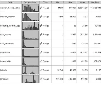
We turn to thehousesdata set [3], which provides census information from all the block groups from the 1990 California census. For this data set, a block group has an average of 1425.5 people living in an area that is geographically compact. Block groups that contained zero entries for any of the variables were excluded.Median house valueis the response variable; the predictor variables are:
r Median income r Population r Housing median age r Households
r Total rooms r Latitude
r Total bedrooms r Longitude
The original data set had 20,640 records, of which 18,540 were selected ran-domly for a training data set, and 2100 held out for a test data set. A quick look at the variables is provided in Figure 1.1. (“Range” is Clementine’s type label for con-tinuous variables.)Median house valueappears to be in dollars, butmedian income has been scaled to a continuous scale from 0 to 15. Note thatlongitudeis expressed in negative terms, meaning west of Greenwich. Larger absolute values for longitude indicate geographic locations farther west.
SPH SPH
JWDD006-01 JWDD006-Larose November 18, 2005 17:46 Char Count= 0
6 CHAPTER 1 DIMENSION REDUCTION METHODS
Figure 1.1 Housesdata set (Clementine data audit node).
is centered between the University of California at Berkeley and Tilden Regional Park.
[image:24.441.52.390.59.341.2]Note from Figure 1.1 the great disparity in variability among the variables. Me-dian incomehas a standard deviation less than 2, whiletotal roomshas a standard devi-ation over 2100. If we proceeded to apply principal components analysis without first standardizing the variables,total roomswould dominatemedian income’s influence,
PRINCIPAL COMPONENTS ANALYSIS 7
and similarly across the spectrum of variabilities. Therefore, standardization is called for. The variables were standardized and theZ-vectors found, Zi =(Xi−µi)/σii, using the means and standard deviations from Figure 1.1.
Note that normality of the data is not strictly required to perform noninferential PCA [4] but that departures from normality may diminish the correlations observed [5]. Since we do not plan to perform inference based on our PCA, we will not worry about normality at this time. In Chapters 2 and 3 we discuss methods for transforming nonnormal data.
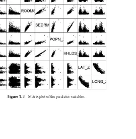
[image:25.441.94.364.312.589.2]Next, we examine the matrix plot of the predictors in Figure 1.3 to explore whether correlations exist. Diagonally from left to right, we have the standardized vari-ablesminc-z(median income),hage-z (housing median age),rooms-z(total rooms), bedrms-z(total bedrooms), popn-z (population), hhlds-z (number of households), lat-z(latitude), andlong-z(longitude). What does the matrix plot tell us about the correlation among the variables? Rooms, bedrooms, population, and households all appear to be positively correlated. Latitude and longitude appear to be negatively correlated. (What does the plot of latitude versus longitude look like? Did you say the state of California?) Which variable appears to be correlated the least with the other predictors? Probablyhousing median age. Table 1.1 shows the correlation matrixρ for the predictors. Note that the matrix is symmetrical and that the diagonal elements all equal 1. A matrix plot and the correlation matrix are two ways of looking at the
SPH SPH
JWDD006-01 JWDD006-Larose November 18, 2005 17:46 Char Count= 0
8 CHAPTER 1 DIMENSION REDUCTION METHODS
TABLE 1.1 Correlation Matrixρ
minc-z hage-z rooms-z bedrms-z popn-z hhlds-z lat-z long-z
minc-z 1.000 −0.117 0.199 −0.012 0.002 0.010 −0.083 −0.012
hage-z −0.117 1.000 −0.360 −0.318 −0.292 −0.300 0.011 −0.107
rooms-z 0.199 −0.360 1.000 0.928 0.856 0.919 −0.035 0.041
bedrms-z −0.012 −0.318 0.928 1.000 0.878 0.981 −0.064 0.064
popn-z 0.002 −0.292 0.856 0.878 1.000 0.907 −0.107 0.097
hhlds-z 0.010 −0.300 0.919 0.981 0.907 1.000 −0.069 0.051
lat-z −0.083 0.011 −0.035 −0.064 −0.107 −0.069 1.000 −0.925
long-z −0.012 −0.107 0.041 0.064 0.097 0.051 −0.925 1.000
same thing: the correlation structure among the predictor variables. Note that the cells for the correlation matrixρline up one to one with the graphs in the matrix plot.
What would happen if we performed, say, a multiple regression analysis of me-dian housing valueon the predictors, despite the strong evidence for multicollinearity in the data set? The regression results would become quite unstable, with (among other things) tiny shifts in the predictors leading to large changes in the regression coefficients. In short, we could not use the regression results for profiling. That is where PCA comes in. Principal components analysis can sift through this correla-tion structure and identify the components underlying the correlated variables. Then the principal components can be used for further analysis downstream, such as in regression analysis, classification, and so on.
Principal components analysis was carried out on the eight predictors in the housesdata set. Thecomponent matrixis shown in Table 1.2. Each of the columns in Table 1.2 represents one of the components Yi =eiZ. The cell entries, called the component weights, represent the partial correlation between the variable and the component. Result 2 tells us that these component weights therefore equal Corr(Yi,Zj)=ei j
√
λi, a product involving theith eigenvector and eigenvalue. Since the component weights are correlations, they range between 1 and−1.
In general, the first principal component may be viewed as the single best summary of the correlations among the predictors. Specifically, this particular linear
TABLE 1.2 Component Matrixa
Component
1 2 3 4 5 6 7 8
minc-z 0.086 −0.058 0.922 0.370 −0.02 −0.018 0.037 −0.004
hage-z −0.429 0.025 −0.407 0.806 0.014 0.026 0.009 −0.001
rooms-z 0.956 0.100 0.102 0.104 0.120 0.162 −0.119 0.015
bedrms-z 0.970 0.083 −0.121 0.056 0.144 −0.068 0.051 −0.083
popn-z 0.933 0.034 −0.121 0.076 −0.327 0.034 0.006 −0.015
hhlds-z 0.972 0.086 −0.113 0.087 0.058 −0.112 0.061 0.083
lat-z −0.140 0.970 0.017 −0.088 0.017 0.132 0.113 0.005
long-z 0.144 −0.969 −0.062 −0.063 0.037 0.136 0.109 0.007
PRINCIPAL COMPONENTS ANALYSIS 9
TABLE 1.3 Eigenvalues and Proportion of Variance Explained by Component
Initial Eigenvalues
Component Total % of Variance Cumulative % 1 3.901 48.767 48.767 2 1.910 23.881 72.648 3 1.073 13.409 86.057 4 0.825 10.311 96.368 5 0.148 1.847 98.215 6 0.082 1.020 99.235 7 0.047 0.586 99.821 8 0.014 0.179 100.000
combination of the variables accounts for more variability than that of any other conceivable linear combination. It has maximized the variance Var(Y1)=e1ρe1. As we suspected from the matrix plot and the correlation matrix, there is evidence that total rooms,total bedrooms,population, andhouseholdsvary together. Here, they all have very high (and very similar) component weights, indicating that all four variables are highly correlated with the first principal component.
Let’s examine Table 1.3, which shows the eigenvalues for each component along with the percentage of the total variance explained by that component. Recall thatresult 3showed us that the proportion of the total variability inZthat is explained by theith principal component isλi/m, the ratio of theith eigenvalue to the number of variables. Here we see that the first eigenvalue is 3.901, and since there are eight predictor variables, this first component explains 3.901/8=48.767% of the variance, as shown in Table 1.3 (allowing for rounding). So a single component accounts for nearly half of the variability in the set of eight predictor variables, meaning that this single component by itself carries about half of the information in all eight predictors. Notice also that the eigenvalues decrease in magnitude,λ1≥λ2≥ · · · ≥λm, λ1≥
λ2≥ · · · ≥λ8,as we noted inresult 2.
The second principal componentY2is the second-best linear combination of the variables, on the condition that it isorthogonalto the first principal component. Two vectors areorthogonalif they are mathematically independent, have no correlation, and are at right angles to each other. The second component is derived from the variability that is left over once the first component has been accounted for. The third component is the third-best linear combination of the variables, on the condition that it is orthogonal to the first two components. The third component is derived from the variance remaining after the first two components have been extracted. The remaining components are defined similarly.
How Many Components Should We Extract?
SPH SPH
JWDD006-01 JWDD006-Larose November 18, 2005 17:46 Char Count= 0
10 CHAPTER 1 DIMENSION REDUCTION METHODS
the first principal component, since it explains nearly half the variability? Or should we retain all eight components, since they explain 100% of the variability? Well, clearly, retaining all eight components does not help us to reduce the number of distinct explanatory elements. As usual, the answer lies somewhere between these two extremes. Note from Table 1.3 that the eigenvalues for several of the components are rather low, explaining less than 2% of the variability in theZ-variables. Perhaps these would be the components we should consider not retaining in our analysis? The criteria used for deciding how many components to extract are (1) the eigenvalue criterion, (2) the proportion of variance explained criterion, (3) the minimum communality criterion, and (4) the scree plot criterion.
Eigenvalue Criterion
Recall from result 1 that the sum of the eigenvalues represents the number of variables entered into the PCA. An eigenvalue of 1 would then mean that the component would explain about “one variable’s worth” of the variability. The rationale for using the eigenvalue criterion is that each component should explain at least one variable’s worth of the variability, and therefore the eigenvalue criterion states that only components with eigenvalues greater than 1 should be retained. Note that if there are fewer than 20 variables, the eigenvalue criterion tends to recommend extracting too few components, while if there are more than 50 variables, this criterion may recommend extracting too many. From Table 1.3 we see that three components have eigenvalues greater than 1 and are therefore retained. Component 4 has an eigenvalue of 0.825, which is not too far from 1, so that if other criteria support such a decision, we may decide to consider retaining this component as well, especially in view of the tendency of this criterion to recommend extracting too few components.
Proportion of Variance Explained Criterion
First, the analyst specifies how much of the total variability he or she would like the principal components to account for. Then the analyst simply selects the components one by one until the desired proportion of variability explained is attained. For exam-ple, suppose that we would like our components to explain 85% of the variability in the variables. Then, from Table 1.3, we would choose components 1 to 3, which together explain 86.057% of the variability. On the other hand, if we wanted our components to explain 90% or 95% of the variability, we would need to include component 4 with components 1 to 3, which together would explain 96.368% of the variability. Again, as with the eigenvalue criterion, how large a proportion is enough?
PRINCIPAL COMPONENTS ANALYSIS 11
of variability explained may be a shade lower than otherwise. On the other hand, if the principal components are to be used as replacements for the original (standard-ized) data set and used for further inference in models downstream, the proportion of variability explained should be as much as can conveniently be achieved given the constraints of the other criteria.
Minimum Communality Criterion
We postpone discussion of this criterion until we introduce the concept ofcommunality below.
Scree Plot Criterion
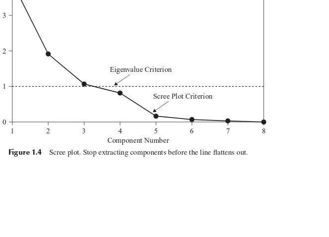
A scree plot is a graphical plot of the eigenvalues against the component number. Scree plots are useful for finding an upper bound (maximum) for the number of components that should be retained. See Figure 1.4 for the scree plot for this example. Most scree plots look broadly similar in shape, starting high on the left, falling rather quickly, and then flattening out at some point. This is because the first component usually explains much of the variability, the next few components explain a moderate amount, and the latter components explain only a small amount of the variability. The scree plot criterion is this: The maximum number of components that should be extracted is just prior towhere the plot first begins to straighten out into a horizontal line. For example, in Figure 1.4, the plot straightens out horizontally starting at component 5.
5
4
3
2
1
0
1 2 3 4 5 6 7 8 Eigenvalue Criterion
Scree Plot Criterion
Component Number
Eigen
v
[image:29.441.57.388.351.590.2]alue
SPH SPH
JWDD006-01 JWDD006-Larose November 18, 2005 17:46 Char Count= 0
12 CHAPTER 1 DIMENSION REDUCTION METHODS
The line is nearly horizontal because the components all explain approximately the same amount of variance, which is not much. Therefore, the scree plot criterion would indicate that the maximum number of components we should extract is four, since the fourth component occurs just prior to where the line first begins to straighten out.
To summarize, the recommendations of our criteria are as follows:
r Eigenvalue criterion. Retain components 1 to 3, but don’t throw component 4 away yet.
r Proportion of variance explained criterion. Components 1 to 3 account for a solid 86% of the variability, and adding component 4 gives us a superb 96% of the variability.
r Scree plot criterion. Don’t extract more than four components.
So we will extract at least three but no more than four components. Which is it to be, three or four? As in much of data analysis, there is no absolute answer in this case to the question of how many components to extract. This is what makes data mining an art as well as a science, and this is another reason why data mining requires human direction. The data miner or data analyst must weigh all the factors involved in a decision and apply his or her judgment, tempered by experience.
In a case like this, where there is no clear-cut best solution, why not try it both ways and see what happens? Consider Table 1.4, which compares the component matrixes when three and four components are extracted, respectively. Component weights smaller than 0.15 are suppressed to ease component interpretation. Note that the first three components are each exactly the same in both cases, and each is the same as when we extracted all eight components, as shown in Table 1.2 (after suppressing the small weights). This is because each component extracts its portion of the variability sequentially, so that later component extractions do not affect the earlier ones.
TABLE 1.4 Component Matrixes for Extracting Three and Four Componentsa
Component Component
1 2 3 1 2 3 4
minc-z 0.922 0.922 0.370
hage-z −0.429 −0.407 −0.429 −0.407 0.806
rooms-z 0.956 0.956
bedrms-z 0.970 0.970
popn-z 0.933 0.933
hhlds-z 0.972 0.972
lat-z 0.970 0.970
long-z −0.969 −0.969
PRINCIPAL COMPONENTS ANALYSIS 13
Profiling the Principal Components
The analyst is usually interested in profiling the principal components. Let us now examine the salient characteristics of each principal component.
r Principal component 1, as we saw earlier, is composed largely of the “block group size” variablestotal rooms,total bedrooms,population, andhouseholds, which are all either large or small together. That is, large block groups have a strong tendency to have large values for all four variables, whereas small block groups tend to have small values for all four variables.Median housing ageis a smaller, lonely counterweight to these four variables, tending to be low (recently built housing) for large block groups, and high (older, established housing) for smaller block groups.
r Principal component 2is a “geographical” component, composed solely of the
latitudeandlongitudevariables, which are strongly negatively correlated, as we can tell by the opposite signs of their component weights. This supports our earlier EDA regarding these two variables in Figure 1.3 and Table 1.1. The negative correlation is because of the way that latitude and longitude are signed by definition, and because California is broadly situated from northwest to southeast. If California were situated from northeast to southwest, latitude and longitude would be positively correlated.
r Principal component 3refers chiefly to themedian incomeof the block group, with a smaller effect due to the housing median age of the block group. That is, in the data set, high median income is associated with recently built housing, whereas lower median income is associated with older, established housing.
r Principal component 4is of interest, because it is the one that we have not decided whether or not to retain. Again, it focuses on the combination ofhousing median ageandmedian income. Here, we see thatonce the negative correlation between these two variables has been accounted for, there is left over a positive relationship between these variables. That is, once the association between, for example, high incomes and recent housing has been extracted, there is left over some further association between high incomes and older housing.
To further investigate the relationship between principal components 3 and 4and their constituent variables, we next consider factor scores.Factor scoresare estimated values of the factors for each observation, and are based onfactor analysis, discussed in the next section. For the derivation of factor scores, see Johnson and Wichern [4].
SPH SPH
JWDD006-01 JWDD006-Larose November 18, 2005 17:46 Char Count= 0
14 CHAPTER 1 DIMENSION REDUCTION METHODS
Figure 1.5 Correlations betweencomponents 3and4and their variables.
component weights, as, for example, 0.922 having a greater amplitude than−0.407 for thecomponent 3component weights. Is this difference in magnitude reflected in the matrix plots?
Consider Figure 1.5a. The strong positive correlation between component 3 andmedian incomeis strikingly evident, reflecting the 0.922 positive correlation. But the relationship betweencomponent 3andhousing median ageis rather amorphous. It would be difficult with only the scatter plot to guide us to estimate the correlation betweencomponent 3andhousing median ageas being−0.407. Similarly, for Fig-ure 1.5b, the relationship betweencomponent 4andhousing median ageis crystal clear, reflecting the 0.806 positive correlation, while the relationship between compo-nent 3andmedian incomeis not entirely clear, reflecting its lower positive correlation of 0.370. We conclude, therefore, that the component weight of−0.407 forhousing median age incomponent 3is not of practical significance, and similarly for the component weight formedian incomeincomponent 4.
This discussion leads us to the following criterion for assessing the compo-nent weights. For a compocompo-nent weight to be considered of practical significance, it should exceed±0.50 in magnitude. Note that the component weight represents the correlation between the component and the variable; thus, the squared component weight represents the amount of the variable’s total variability that is explained by the component. Thus, this threshold value of±0.50 requires that at least 25% of the variable’s variance be explained by a particular component. Table 1.5 therefore presents the component matrix from Table 1.4, this time suppressing the component weights below±0.50 in magnitude. The component profiles should now be clear and uncluttered:
PRINCIPAL COMPONENTS ANALYSIS 15
TABLE 1.5 Matrix of Component Weights, Suppressing Magnitudes Below±0.50a
Component
1 2 3 4
minc-z 0.922
hage-z 0.806
rooms-z 0.956
bedrms-z 0.970
popn-z 0.933
hhlds-z 0.972
lat-z 0.970
long-z −0.969
aExtraction method: principal component analysis; four components extracted.
r Principal component 2represents the “geographical” component and consists of two variables,latitudeandlongitude.
r Principal component 3represents the “income” component and consists of only one variable,median income.
r Principal component 4represents the “housing age” component and consists of only one variable,housing median age.
Note that the partition of the variables among the four components ismutually exclusive, meaning that no variable is shared (after suppression) by any two com-ponents, andexhaustive, meaning that all eight variables are contained in the four components. Further, support for this 4–2–1–1 partition of the variables among the first four components is found in the similar relationship identified among the first four eigenvalues: 3.901–1.910–1.073–0.825 (see Table 1.3).
A note about positive and negative loadings is in order. Considercomponent 2, which has a strong positive loading forlatitudeand a strong negative loading for longitude. It is possible that a replication study would find that the signs for these loadings would be reversed, so thatlatitudehad a negative loading andlongitudehad a positive loading. If so, the interpretation is exactly the same, because we interpret the relationship between the variables rather than the signs per se.
Communalities
We are moving toward a decision regarding how many components to retain. One more piece of the puzzle needs to be set in place:communality. PCA does not extract all the variance from the variables, only that proportion of the variance that is shared by several variables. Communality represents the proportion of variance of a particular variable that is shared with other variables.
SPH SPH
JWDD006-01 JWDD006-Larose November 18, 2005 17:46 Char Count= 0
16 CHAPTER 1 DIMENSION REDUCTION METHODS
among the variables and contributes less to the PCA solution. Communalities that are very low for a particular variable should be an indication to the analyst that the particular variable might not participate in the PCA solution (i.e., might not be a member of any of the principal components). Overall, large communality values indicate that the principal components have successfully extracted a large proportion of the variability in the original variables; small communality values show that there is still much variation in the data set that has not been accounted for by the principal components.
Communality values are calculated as the sum of squared component weights for a given variable. We are trying to determine whether to retaincomponent 4, the “housing age” component. Thus, we calculate the commonality value for the variable housing median age, using the component weights for this variable (hage-z) from Table 1.2. Two communality values forhousing median ageare calculated, one for retaining three components and the other for retaining four components.
r Communality (housing median age, three components):
(−0.429)2+(0.025)2+(−0.407)2=0.350315 r Communality (housing median age, four components):
(−0.429)2+(0.025)2+(−0.407)2+(0.806)2=0.999951
Communalities less than 0.5 can be considered to be too low, since this would mean that the variable shares less than half of its variability in common with the other variables. Now, suppose that for some reason we wanted or needed to keep the variablehousing median ageas an active part of the analysis. Then, extracting only three components would not be adequate, sincehousing median ageshares only 35% of its variance with the other variables. If we wanted to keep this variable in the analysis, we would need to extract the fourth component, which lifts the communality forhousing median ageover the 50% threshold. This leads us to the statement of the minimum communality criterionfor component selection, which we alluded to earlier.
Minimum Communality Criterion
Suppose that it is required to keep a certain set of variables in the analysis. Then enough components should be extracted so that the communalities for each of these variables exceeds a certain threshold (e.g., 50%).
Hence, we are finally ready to decide how many components to retain. We have decided to retain four components, for the following reasons:
r The eigenvalue criterion recommended three components but did not absolutely reject the fourth component. Also, for small numbers of variables, this criterion can underestimate the best number of components to extract.
PRINCIPAL COMPONENTS ANALYSIS 17
and use them in further modeling downstream, being able to explain so much of the variability in the original data is very attractive.
r The scree plot criterion said not to exceed four components. We have not. r The minimum communality criterion stated that if we wanted to keephousing
median agein the analysis, we had to extract the fourth component. Since we intend to substitute the components for the original data, we need to keep this variable, and therefore we need to extract the fourth component.
Validation of the Principal Components
Recall that the original data set was divided into a training data set and a test data set. All of the analysis above has been carried out on the training data set. To validate the principal components uncovered here, we now perform PCA on the standardized variables for the test data set. The resulting component matrix is shown in Table 1.6, with component weights smaller than±0.50 suppressed. Although the component weights do not exactly equal those of the training set, the same four components were extracted, with a one-to-one correspondence in terms of which variables are associated with which component. This may be considered validation of the principal components analysis performed. Therefore, we shall substitute these principal compo-nents for the standardized variables in our later analysis on this data set. Specifically, we investigate whether the components are useful for estimating themedian house value.
If the split-sample method described here does not successfully provide vali-dation, the analyst should take this as an indication that the results (for the data set as a whole) are not generalizable, and the results should not be reported as valid. If the lack of validation stems from a subset of the variables, the analyst may consider omitting these variables and performing the principal components analysis again. An example of the use of principal component analysis in multiple regression is provided in Chapter 3.
TABLE 1.6 Validating the PCA: Matrix of Component Weights for the Test Seta
Component
Variables 1 2 3 4
minc-z 0.920
hage-z 0.785
rooms-z 0.957
bedrms-z 0.967
popn-z 0.935
hhlds-z 0.968
lat-z 0.962
long-z −0.961
SPH SPH
JWDD006-01 JWDD006-Larose November 18, 2005 17:46 Char Count= 0
18 CHAPTER 1 DIMENSION REDUCTION METHODS
FACTOR ANALYSIS
Factor analysis is related to principal components, but the two methods have different goals. Principal components seeks to identify orthogonal linear combinations of the variables, to be used either for descriptive purposes or to substitute a smaller number of uncorrelated components for the original variables. In contrast, factor analysis represents amodelfor the data, and as such is more elaborate.
Thefactor analysis modelhypothesizes that the response vector X1,X2, . . . , Xmcan be modeled as linear combinations of a smaller set ofkunobserved, “latent” random variables F1,F2, . . . ,Fk, called common factors, along with an error term
ε=ε1, ε2, . . . , εk.Specifically, the factor analysis model is
X−µ
m×1 =mL×k kF×1 +mε×1 whereX−µ
m×1
is the response vector, centered by the mean vector; L
m×k
is the matrix offactor loadings, withli jrepresenting the factor loading of theith variable on the
jth factor; F
k×1
represents the vector of unobservable common factors and ε m×1 the error vector. The factor analysis model differs from other models, such as the linear regression model, in that thepredictor variables F1,F2, . . . ,Fk are unobservable. Because so many terms are unobserved, further assumptions must be made before we may uncover the factors from the observed responses alone. These assumptions are thatE(F)=0,Cov(F)=I,E(ε)=0,and Cov(ε) is a diagonal matrix. See Johnson and Wichern [4] for further elucidation of the factor analysis model.
Unfortunately, the factor solutions provided by factor analysis are not invari-ant to transformations. Two models,X−µ=L F+εandX−µ=(LT) (TF)+ε, whereTrepresents an orthogonal transformations matrix, will both provide the same results. Hence, the factors uncovered by the model are in essence nonunique, without further constraints. This indistinctness provides the motivation for factor rotation, which we will examine shortly.
Applying Factor Analysis to the
Adult
Data Set
FACTOR ANALYSIS 19
TABLE 1.7 Correlation Matrix for the Factor Analysis Example
age-z dem-z educ-z capnet-z hours-z
age-z 1.000 −0.076∗∗ 0.033∗∗ 0.070∗∗ 0.069∗∗
dem-z −0.076∗∗ 1.000 −0.044∗∗ 0.005 −0.015∗
educ-z 0.033∗∗ −0.044∗∗ 1.000 0.116∗∗ 0.146∗∗
capnet-z 0.070∗∗ 0.005 0.116∗∗ 1.000 0.077∗∗
hours-z 0.069∗∗ −0.015∗ 0.146∗∗ 0.077∗∗ 1.000
∗∗Correlation is significant at the 0.01 level (two-tailed). ∗Correlation is significant at the 0.05 level (two-tailed).
To function appropriately, factor analysis requires a certain level of correla-tion. Tests have been developed to ascertain whether there exists sufficiently high correlation to perform factor analysis.
r The proportion of variability within the standardized predictor variables which is shared in common, and therefore might be caused by underlying factors, is measured by theKaiser–Meyer–Olkin measure of sampling adequacy. Values of the KMO statistic less than 0.50 indicate that factor analysis may not be appropriate.
r Bartlett’s test of sphericitytests the null hypothesis that the correlation matrix is an identity matrix, that is, that the variables are really uncorrelated. The statis-tic reported is thep-value, so that very small values would indicate evidence against the null hypothesis (i.e., the variables really are correlated). Forp-values much larger than 0.10, there is insufficient evidence that the variables are not uncorrelated, so factor analysis may not be suitable.
Table 1.8 provides the results of these statistical tests. The KMO statistic has a value of 0.549, which is not less than 0.5, meaning that this test does not find the level of correlation to be too low for factor analysis. Thep-value for Bartlett’s test of sphericity rounds to zero, so that the null hypothesis that no correlation exists among the variables is rejected. We therefore proceed with the factor analysis.
To allow us to view the results using a scatter plot, we decide a priori to extract only two factors. The following factor analysis is performed using theprincipal axis factoringoption. In principal axis factoring, an iterative procedure is used to estimate the communalities and the factor solution. This particular analysis required 152 such iterations before reaching convergence. The eigenvalues and the proportions of the variance explained by each factor are shown in Table 1.9. Note that the first two factors
TABLE 1.8 Is There Sufficiently High Correlation to Run Factor Analysis?
Kaiser–Meyer–Olkin measure of sampling adequacy 0.549 Bartlett’s test of sphericity
Approx. chi-square 1397.824 degrees of freedom (df) 10
SPH SPH
JWDD006-01 JWDD006-Larose November 18, 2005 17:46 Char Count= 0
20 CHAPTER 1 DIMENSION REDUCTION METHODS
TABLE 1.9 Eigenvalues and Proportions of Variance Explained: Factor Analysisa
Initial Eigenvalues
Factor Total % of Variance Cumulative %
1 1.277 25.533 25.533 2 1.036 20.715 46.248 3 0.951 19.028 65.276 4 0.912 18.241 83.517 5 0.824 16.483 100.000
aExtraction method: principal axis factoring.
extract less than half of the total variability in the variables, as contrasted with the housesdata set, where the first two components extracted over 72% of the variability. This is due to the weaker correlation structure inherent in the original data.
Thefactor loadings L
m×kare shown in Table 1.10. Factor loadings are analogous to the component weights in principal components analysis and represent the corre-lation between theith variable and the jth factor. Notice that the factor loadings are much weaker than the previoushousesexample, again due to the weaker correlations among the standardized variables. The communalities are also much weaker than the housesexample, as shown in Table 1.11. The low communality values reflect the fact that there is not much shared correlation among the variables. Note that the factor extraction increases the shared correlation.
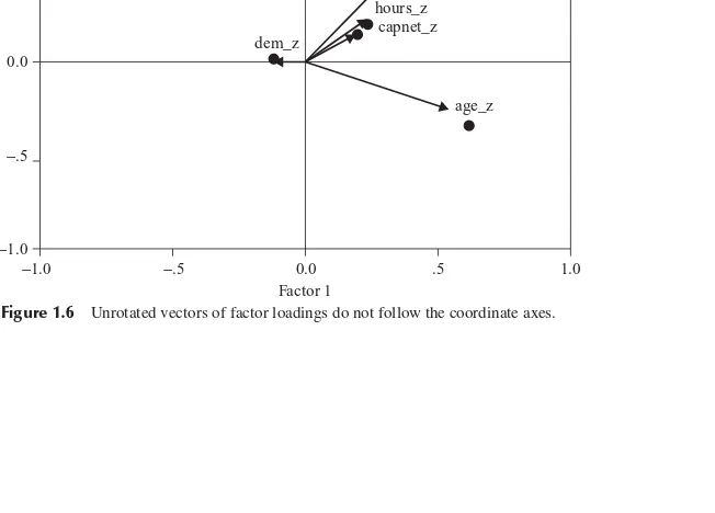
Factor Rotation
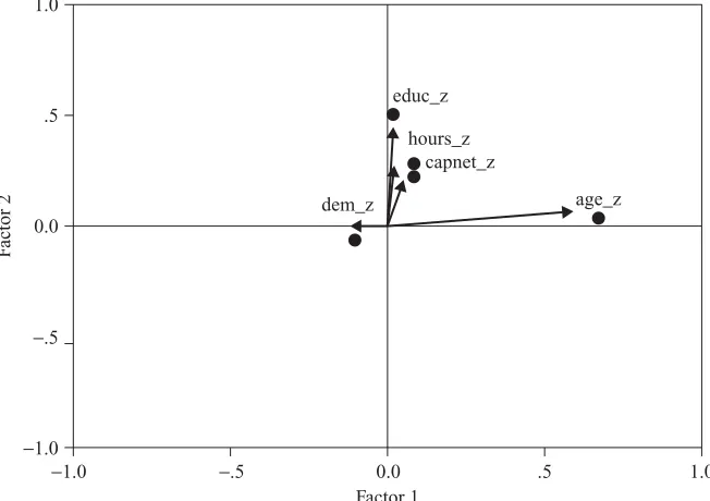
To assist in the interpretation of the factors,factor rotationmay be performed. Factor rotation corresponds to a transformation (usually, orthogonal) of the coordinate axes, leading to a different set of factor loadings. We may look upon factor rotation as analogous to a scientist attempting to elicit greater contrast and detail by adjusting the focus of a microscope.
The sharpest focus occurs when each variable has high factor loadings on a single factor, with low to moderate loadings on the other factors. For thehouses example, this sharp focus already occurred on the unrotated factor loadings (e.g.,
TABLE 1.10 Factor Loadingsa
Factor
1 2
age-z 0.590 −0.329
educ-z 0.295 0.424
capnet-z 0.193 0.142
hours-z 0.224 0.193
dem-z −0.115 0.013