EVALUATION OF SPATIAL AND TEMPORAL PATTERNS OF PRIORITY CONTAMINANTS IN SEDIMENTS OF THE HURON-ERIE CORRIDOR

(1)

University of Windsor University of Windsor

Scholarship at UWindsor

Electronic Theses and Dissertations Theses, Dissertations, and Major Papers

2017

EVALUATION OF SPATIAL AND TEMPORAL PATTERNS OF

PRIORITY CONTAMINANTS IN SEDIMENTS OF THE HURON-ERIE

CORRIDOR

Joseph LaFontaine University of Windsor

Follow this and additional works at: https://scholar.uwindsor.ca/etd

Recommended Citation Recommended Citation

LaFontaine, Joseph, "EVALUATION OF SPATIAL AND TEMPORAL PATTERNS OF PRIORITY CONTAMINANTS IN SEDIMENTS OF THE HURON-ERIE CORRIDOR" (2017). Electronic Theses and Dissertations. 5993.

https://scholar.uwindsor.ca/etd/5993

(2)

EVALUATION OF SPATIAL AND TEMPORAL PATTERNS OF PRIORITY

CONTAMINANTS IN SEDIMENTS OF THE HURON-ERIE CORRIDOR

By

Joseph LaFontaine

A Thesis

Submitted to the Faculty of Graduate Studies

Through the Great Lakes Institute for Environmental Research

In Partial Fulfillment of the Requirements for

The Degree of Master of Science at the University of Windsor

Windsor, Ontario, Canada

(3)

Evaluation of spatial and temporal patterns of priority contaminants in sediments of the Huron-Erie Corridor

By

Joseph LaFontaine

Approved By:

J.J.H Ciborowski Biological Sciences

J.E. Gagnon

GLIER, Earth and Environmental Sciences

G.D. Haffner GLIER

K.G. Drouillard, Advisor GLIER

(4)

DECLARATION OF CO-AUTHORSHIP

I hereby declare that this thesis incorporates material that is result of joint research, as follows: Chapters 2 and 3 of this thesis will be published as co-authored, peer-reviewed journal articles. Chapter 2 is being prepared for submission to Chemosphere with co-authorship with Alice-Ggicak-Mannion and Ken Drouillard. Chapter 3 is being prepared for submission and will include co-authors: Ewa Szalinska, Alice Grgicak-Mannion, Kerry McPhedran, Ken G. Drouillard, Ted Briggs and G. Douglas Haffner. The latter co-authors contributed to the previous studies which generated data utilized in Chapter 3, contributed to funding support and editorial review of works completed. Alice Grgicak-Mannion, Kerry McPhedran and Ken G. Drouillard contributed to the experimental design and sampling of portions of the 2013-2014 survey data used in both chapters. I contributed to the sample collection of samples from St. Clair River and Lake St. Clair in the 2013-2014 survey used in Chapter 2 and 3, the complete analytical chemistry workup, database generation and quality assurance/quality control aspects of the 2013-2014 survey data. I also led the data interpretation and writing of all chapters in this thesis with editorial contributions contributed by the above stated co-authors.

I am aware of the University of Windsor Senate Policy on Authorship and I certify that I have properly acknowledged the contribution of other researches to my thesis, and have obtained written permission from each of the co-author(s) to include the above materials in my thesis.

I declare that, to the best of my knowledge, my thesis does not infringe upon anyone’s copyright nor violate any proprietary rights and that any ideas, techniques, quotations, or any other material from the work of other people included in my thesis, published or otherwise, are fully acknowledged in accordance with the standard referencing practices. Furthermore, to the extent that I have included copyrighted material that surpasses the bounds of fair dealing within the meaning of the Canada Copyright Act, I certify that I have obtained a written permission from the copyright owner(s) to include such material(s) in my thesis.

(5)

ABSTRACT

This thesis examined spatial and temporal patterns of sediment contamination within the Huron-Erie Corridor which consists of two Areas of Concern, the St. Clair River and the Detroit River. Stratified random sampling designs of surficial sediment samples, both current (2013-2014) and past (1999-2005), were used to evaluate contamination patterns as well as trends observed in time. Chapter 2 focused on Mercury (Hg)

(6)

ACKNOWLEDGEMENTS

I would like to extend tremendous thanks to my supervisor, Ken Drouillard for

his guidance and sharing of a diverse set of skills throughout the scope of the project.

This project necessitated a number of diverse skills and I am thankful Ken could both

extend my knowledge and provide assistance on everything from project design to boat

navigation to statistical analysis and rigorous writing consultation. I would also like to

thank Nargis Ismail very much for her intense knowledge on organics analytical

chemistry. Nargis went above and beyond requirements to help me learn all the steps to

generate organic analytical concentration data and provided extra assistance when I

was overwhelmed by such a large dataset. Additionally, I would like to thank Alice

Grgicak-Mannion for her continued support, knowledge and assistance and for loaning

her time towards expansion of my GIS knowledge and skillset. David Qiu and JC Barrette

for their technical assistance and lab analysis help. My committee members Jan

Ciborowski, Joel Gagnon and Doug Haffner for generously giving their time to improve

and review my thesis. The following should also be thanked for survey, laboratory and

general help: Joe Robinet, Todd Leadley, Stefan Grigorakis, Bronson Goodfellow as well

as many other GLIER students, staff and summer students.

I also give a special thanks to my Mom and Dad for their unending support

throughout my academic career as well as to my friends who continually support me

(7)

LIST OF TABLES

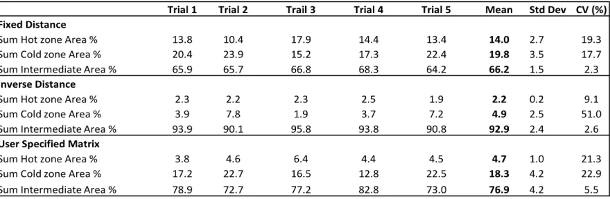
Table 2.1 Total area for each method expressed as percent of total. Mean and Standard

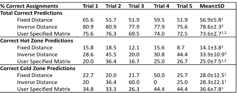
deviation expressed for 5 subsets. ... 30 Table 2.2 Validation expected vs observed results. ... 37

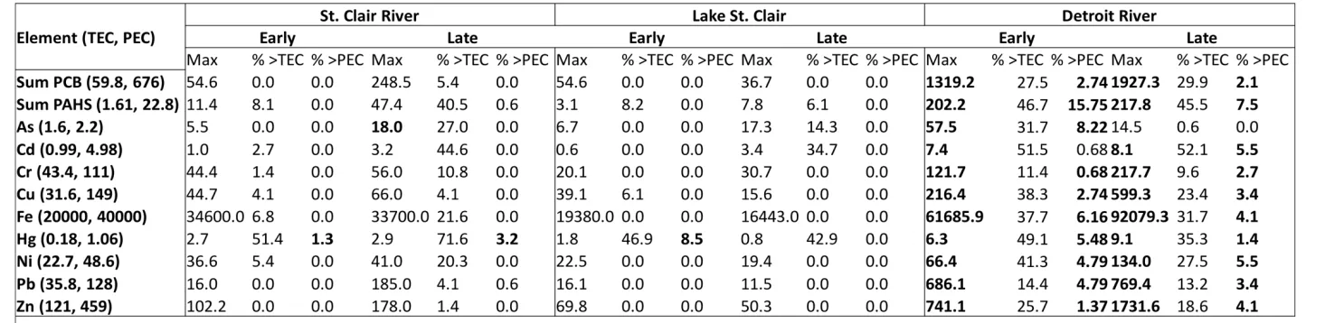
Table 3.1 Max concentrations and Probable effect concentration (PEC) exceedences by

each waterbody and the early and late time period. Concentrations are expressed in ug/g dry weight for metals and PAHs and ng/g for PCBs. ... 67

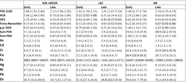
Table 3.2 Priority Contaminant concentrations by waterbody for the Huron-Erie Corridor

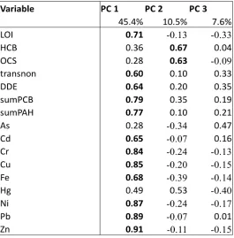
separated by the early and late time periods. Concentrations are expressed as a geometric mean and 95% confidence interval in ug/g dry weight for metals and PAHs and ng/g for PCBs ... 68 Table 3.3 Principal component loadings of contaminants for all years Huron-Erie

corridor dataset. ... 71 Table 3.4 Mass Balance for selected priority contaminants in the surficial sediment of

(9)

LIST OF FIGURES

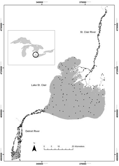
Figure 2.1 Study area, Location of sampling locations from all 6 surveys. ... 20

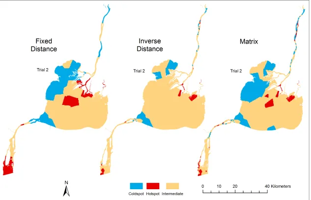
Figure 2.2 Map Comparison of Hot and Cold Zones generated for Trial 2. Red, blue and

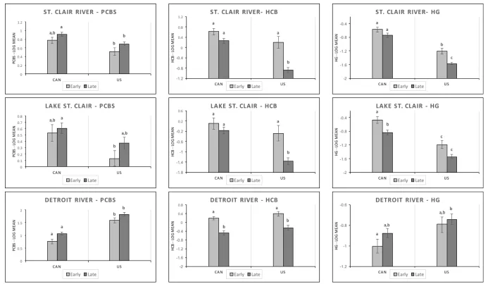
beige designate hot, cold and intermediate zones. ... 32 Figure 3.1 GLM contrasts for PCBs (left graphics), HCB (center graphics) and Hg (right

graphics) separated by waterbody. Within a graphic, different letter subscripts represent significant differences( p < 0.01, GLM) ... 72 Figure 3.2 Hot and Cold zone contrasts with sample locations included for the Early and

Late time periods for PCBs. Red Ellipses represent common hot zones between time periods, blue ellipses represent common cold zones between time periods. . 79 Figure 3.3 Hot and Cold zone contrasts with sample locations included for the Early and

Late time periods for HCB. Red Ellipses represent common hot zones between time periods, blue ellipses represent common cold zones between time periods. Dashed ellipse represent a difference between sample years ... 80 Figure 3.4 Hot and Cold zone contrasts with sample locations included for the Early and

Late time periods for Hg. Red Ellipses represent common hot zones between time periods, blue ellipses represent common cold zones between time periods. Dashed ellipse represents a difference between sample years ... 81 Figure 3.5 Hot and Cold zone contrasts with sample locations included for the Early and

(10)

CHAPTER 1 – GENERAL INTRODUCTION

1.1 – General Introduction

Agricultural and industrial processes coupled with rising human populations and the

spread of globalization have led to sediment contamination being found in almost all

water systems worldwide (Reynoldson and Zarull, 1989). One of these freshwater areas

under particular environmental stress is the Laurentian Great Lakes (Grapentine, 2009).

As human impacts on the environment continue to grow, the need for the management

of ecosystem and water quality of one of the largest freshwater areas in the world

becomes increasingly crucial (Cairns Jr. et al., 1993; Nobi et al., 2010). Both Canada and

the United States have recognized this importance and beginning in 1972 the Great

Lakes Water Quality Agreement (GLWQA) was signed. There have since been 42 Areas

of Concern (AOCs) designated within the Great Lakes as a result of one or more

designated impaired beneficial uses as specified by the International Joint Commission

(IJC, 1987).

Within the Laurentian Great Lakes is the Huron Erie Corridor (HEC) consisting of the

St. Clair River, Lake St. Clair and the Detroit River. At 157 km in length, it is the main

connecting waterway between Lake Huron and Lake Erie. This system is particularly

complex, consisting of two riverine systems, one deltaic and one lake system(Szalinska

et al., 2007). The corridor serves as the international border between the United States

and Canada and runs through agricultural, along with highly urbanized and

industrialized areas resulting in a complex history of contamination from a variety of

(11)

the Detroit River are designated Great Lakes Areas of Concern (AOCs), with two

additional AOCs the Clinton River and the Rouge River flowing into the system. Both the

Detroit River and St. Clair River Remedial Action Plans identified upwards of 10

beneficial use impairments each including but not limited to degradation of benthos,

loss of fish and wildlife habitat, degradation of fish and wildlife populations, restrictions

on fish consumption and beach closings (DRCCC, 2009; Szalinska et al., 2007; US EPA,

2013a, 2013b). There has been widespread monitoring, mainly within specific reaches of

the corridor, throughout the past 30 years(Szalinska et al., 2007; US EPA, 2013a).

A beneficial use impairment (BUI) is defined as a use that has been compromised

due to a change in chemical, physical or biological integrity within a system. There are a

total of 14 standardized use impairments used and assessed across the AOC’s (IJC,

1987). The Detroit River was allocated a 15th beneficial use impairment with respect to

exceedances of water quality standards. Sediment contamination itself is a factor

directly related to a number of BUIs identified in the HEC. Accumulation of a variety of

pollutants in sediments led to the degradation of ecosystem health, accumulation of

contaminants in tissues of benthic organisms and fishes, along with drinking water

restrictions and restrictions of dredging activities(Richman and Milani, 2010). Due to

this, the evaluation of sediment chemistry has long been used to monitor contaminant

levels and their respective locations throughout the HEC. Historically, the St. Clair River

and Detroit River have been of greater focus in studies (Oliver and Bourbonniere, 1985;

(12)

adapted to studying Lake St. Clair along with the corridor as a system (Szalinska et al.,

2007).

A number of complex factors govern the spread of contaminants within large

systems such as the HEC. A contaminant is defined as a chemical enriched by

anthropogenic activities, though it may not necessarily cause harm. Contaminants

through initial release are transported by being a) dissolved into the water phase, b)

partitioned/adsorbed onto particles and then transported via suspended sediments, or

c) by the movement of the bedload, i.e. downstream transport of sediments along the

river bottom(Drouillard et al., 2006; Lau et al., 1989). Contaminants associated with

scavenged particles have been shown to be deposited and accumulate in areas where

the water current can no longer sustain particle transport (Szalinska et al., 2011). The

HEC consists of altered flow in channels and variable deposition zones (both nearshore

and deltaic) that contribute to a high variation of particle size distributions, and

sediment consolidation and composition differences(Szalinska et al., 2013). Differences

in particle size, organic carbon and mineral content can influence the concentration and

type of contaminants that can be found to load or accumulate together. Organic matter

has been shown to retain organic contaminants (Hawker and Connell, 1988) while the

finer clay fraction has been observed to preferentially retain metal and metalloid

particles (Golterman, 2004). These geochemical variables, coupled with diverse

input/source locations, contribute to high heterogeneity of contaminant patterns in

sediments beyond what is observed compared to more homogeneous environmental

(13)

Current and historical anthropogenic activities has also been found to influence the

dispersion and location of contaminants found in sediments (Szalinska et al., 2011). The

HEC being a major trading and shipping route is one of the most heavily industrialized

and environmentally altered areas in the Great Lakes (Szalinska et al., 2011). There is

variation in the stresses placed along the corridor, with specific zones exhibiting greater

concentration of industry than others. The St. Clair River has a heavy industry presence

found on the Upper/Midstream Canadian side, whereas the Detroit River is governed by

two large metropolitan areas, Detroit and Windsor, as well as industry along the U.S.

midstream portion. Anthropogenic sources associated with the above locations were

shown by Szalinska et al., 2011 to have a greater impact on the distribution patterns of

contaminants than the geochemical sorting processes in sections of the HEC. The

localized areas of contaminants identified in the study corresponded with the areas of

industry leading to location and sources as a justifiable factor in contaminated sediment

distribution patterns within the HEC.

The long history of contamination throughout the HEC and the AOC designation led

to the implementation of Remedial Action Plans (RAP). These were put into place to

provide goals to improve the state of the system over time. The extent of sediment

contamination was one of the main focuses of the clean-up effort outlined in the RAP

(Zarull et al., 2001). Sediment contamination has been intensively studied throughout

the corridor over the last thirty years with earlier studies identifying problem areas

within the river systems (Besser et al., 1996; Hamdy and Post, 1985; Pugsley et al.,

(14)

channel showed elevated concentrations of multiple contaminants. Additionally, the

identification of high levels of historical contaminants downstream of Sarnia’s Chemical

Valley on the Canadian side (Szalinska et al., 2007) led to large-scale sediment clean-up

activities. Since 1993 over 1 million cubic meters of contaminated sediments have been

removed from the Detroit River at a cost of over 150$ million dollars (U.S.) (Hartig et al.,

2004). There has been over $200 million (U.S.) spent on the improvement of sewage

treatment and wastewater facilities in both countries. Additionally, the remediation of

roughly 14,000 cubic meters of contaminated sediments was completed by Dow

Chemical adjacent to their property in the St. Clair River (US EPA, 2013b).

These clean-up activities have led to concentration decreases observed through post

monitoring activities, though the extent of such actions to the system recovery as a

whole has not been demonstrated since post-mitigation monitoring work has been

typically constrained to the area of clean up (Szalinska et al., 2013). Still, through the

extensive work completed on the system over time there have been noticeable

improvements, with 5 BUIs removed in the St. Clair River and 2 BUIs in the Detroit River

(US EPA, 2013a, 2013b).

Though clean-up efforts and monitoring have resulted in significant improvements

with time the studies that were taking place were failing to provide the context of

improvement at the corridor wide scale (Szalinska et al., 2013). There were two main

problems with the studies taking place. These studies were often biased towards

locations of point sources or previously identified areas of degradation (Haffner et al.,

(15)

health. Beyond just localization and time events, studies were generally structured to

evaluate a few specific target contaminants or problems in that area. Studies were not

structured to be representative of each other in a timely and spatially relevant sequence

that could account for historical trends and system-wide changes (Haffner et al., 2000;

Szalinska et al., 2006).

A structured, large-scale study implemented to answer the question of whether the

state of the system was improving for the Detroit River AOC was completed in 1999

(Drouillard et al., 2006; Szalinska et al., 2006). That survey sampled 150 stations within

the boundaries of the AOC according to a stratified random geostatistical design. Each

sample location generated bulk sediment chemistry data for metals and priority organic

pollutants to serve as a baseline for contaminant levels within the river. This study was

set apart from previous studies in two main factors: 1) the extent of sediment chemistry

parameters analyzed and 2) the sampling design and implementation of a random

stratified sampling approach which encompassed all waters within the AOC boundary.

The sediment chemistry parameters implemented above included grain size,

moisture content, total organic carbon, and a suite of contaminants that included

metals, PCBs and PAHs previously identified as priority contaminants within the HEC.

This allowed a complete dataset which can lead to understanding sediment dynamics

and to determine which contaminants were grouping together in specific locations

(Drouillard et al., 2006; McPhedran et al., 2016; Szalinska et al., 2006). The sampling

design utilized a stratified random sampling approach. With 150 sample locations, this

(16)

Canadian waters, but also limited sampling of sediments in the dredged navigational

channels. Clustering was taken into account by ensuring that adjacent sample locations

were no closer than 300 m to one another. The survey helped to identify contaminated

areas, evaluate the state of the system and helped to show the differences in

environmental health of the river through the comparison of sediment chemistry results

with Sediment Quality Guidelines (SQGs). Following the 1999 Detroit River study, the

sampling design was expanded for an additional survey in 2004 that encompassed the

HEC with 108 sites sampled throughout its waters (Szalinska et al., 2007). This

established the first survey for the St. Clair River and Lake St. Clair and allowed a

contrast between contaminated systems and the different AOCs of the HEC. Additional

sediment surveys were completed within the Walpole Island Delta (2005, 2012)

encompassing a total of 87 sites, and in the Detroit River in 2008/09 covering 65 sites

(Szalinska et al., 2013).

Technological advances have changed the way we map, design and evaluate the

distribution environmental attributes. The use of Geographic Information Systems (GIS)

make geostatistical analysis of large-scale datasets easier and more manageable.

Recently, following the successes of the large-scale surveys throughout the corridor,

there has been some work to develop hazard zones of contaminants using GIS software.

The study by Szalinska et al., 2013 applied GIS approaches to interpret temporal and

spatial changes observed on the 1999 and 2008/09 Detroit River studies that included

mass balance, along with regional and local geospatial assessment techniques. One

(17)

Statistic measures how spatial autocorrelation varies locally over a study area and

computes a new statistic for each data point that takes into consideration weighted

concentrations at individual sampling stations and places these into the context of the

system-wide mean concentration (ESRI, 2016). The method evaluates the degree to

which a point and its neighbours exhibit similarly high or low values in contamination

compared to the system mean concentration for a given contaminant. Output values

are defined as z-scores, with high positive values indicating a hotspot (i.e. distance

weighted concentrations significantly elevated above the system mean), whereas

negative values indicate a cold spot (locations having distance weighted concentrations

significantly lower than the system mean). The method allows for the localization of hot

and cold spot zones within the Detroit River by identifying clusters of sites that are

above and below the mean contamination for the system. The study coupled hotspot

analysis with mass balance and principal component analysis techniques in order to

evaluate if changes in the overall contamination, regional contamination and localized

hot/cold spots have been observed in the Detroit River over the previous ten-year

period. This was the first step in taking baseline surveys to evaluate if the system was

improving over time.

The implementation of large-scale studies across multiple survey years as

demonstrated within the Detroit River has allowed for greater understanding of the

state of this Area of Concern. Advanced geospatial analysis techniques implemented in

the Detroit River have begun to characterize temporal changes in contaminant

(18)

implemented at the corridor scale. Furthermore, understanding the interactions and

groupings of multiple contaminants at sampling sites can help to understand where

multi-contaminant hotspots exist that can further shed light into potential source

regions and sediment-associated toxicity.

1.2 – Thesis Objectives

This thesis will address a comprehensive geospatial analysis of priority pollutants in

sediments distributed in the Huron Erie corridor. The research has the following

objectives:

Chapter 2 of this thesis assessed the most appropriate method for applying the

Getis-ord statistic in the Huron-Erie Corridor. This objective was addressed by focusing

on total mercury as a priority contaminant due to its anthropgenic nature and well

defined history of study in the Huron-Erie Corridor. Previous application of the

Getis-Ord statistic to the Detroit River (Szalinska et al. 2013) utilized a fixed distance approach

to define which sample neighbours have influence for a given location. However, this

approach considered all points within the defined distance as equal and did not weight

them based on their actual physical connectivity to one another. Furthermore, it did not

consider that directional water flow within the connecting channels places constraints

on sediment mixing probabilities and therefore could lead to inappropriate allocation of

hot and/or cold spots within the system as a result of incorporating neighbor sampling

sites in the weighted Getis-Ord statistic. This thesis research was developed to compare

(19)

inverse distance weighting and a new user defined matrix that considers hydraulic and

island barriers) to describe mercury contamination in sediments of the Huron-Erie

corridor. It was hypothesized that methods that account for distance weighting and/or

account for physical and hydraulic barriers will provide a more accurate estimate of hot

and cold regions.

Chapter 3 of this thesis was developed to provide the first temporal assessment

of multi-pollutant sediment contamination at the corridor scale within the HEC. Building

from the methodology generated in Szalinkska et al. (2013) applied to the Detroit River

and incorporating the results of Chapter 2 on Getis-Ord statistic optimization, Chapter 3

of this thesis evaluated the mass balance, regional, and local changes in sediment

contamination for priority pollutants in the HEC from 1999 to 2014. This chapter tested

whether or not changes in the magnitude and location of priority contaminants in

sediments have occurred within the system over the past decade and whether similar

patterns of change are apparent across multiple contaminants. It was hypothesized that

contamination will have decreased in specific reaches of the corridor such as the Detroit

River U.S. side and St. Clair River Canadian side due to remediation activities designed to

mitigate legacy deposits. It was expected that zones of low contamination would remain

(20)

1.3 - References

Besser, J.M., Giesy, J.P., Kubitz, J.A., Verbrugge, D.A., Coon, T.G., Emmett Braselton, W., 1996. Assessment of Sediment Quality in Dredged and Undredged Areas of the Trenton Channel of the Detroit River, Michigan USA, using the Sediment Quality Triad. J. Great Lakes Res. 22, 683–696. doi:10.1016/S0380-1330(96)70989-9

Cairns Jr., J., McCormick, P., Niederlehner, B.R., 1993. A proposed framework for developing indicators of ecosystem health. Hydrobiologia 263, 1–44.

doi:10.1007/bf00006084

DRCCC, 2009. Detroit River Canadian Cleanup Committee, Detroit River Remedial Action Plan Stage 2 Report, Draft 2009.

Drouillard, K.G., Tomczak, M., Reitsma, S., Haffner, G.D., 2006. A River-wide Survey of Polychlorinated Biphenyls (PCBs), Polycylic Aromatic Hydrocarbons (PAHs), and Selected Organochlorine Pesticide Residues in Sediments of the Detroit River— 1999. J. Great Lakes Res. 32, 209–226.

doi:10.3394/0380-1330(2006)32[209:ARSOPB]2.0.CO;2

ESRI, 2016. How Hot Spot Analysis (Getis-Ord Gi*) works [WWW Document]. URL http://pro.arcgis.com/en/pro-app/tool-reference/spatial-statistics/h-how-hot-spot-analysis-getis-ord-gi-spatial-stati.htm

Golterman, H.., 2004. The Chemistry of Phosphate and Nitrogen Compounds in Sediments. Kluwer Acad. Publ. 251.

Grapentine, L.C., 2009. Determining degradation and restoration of benthic conditions for Great Lakes Areas of Concern. J. Great Lakes Res. 35, 36–44.

doi:10.1016/j.jglr.2008.09.002

Haffner, G.D., Wood, S., Grgicak-manion, A., 2000. Design and interpretation of toxic chemical distribution and stress : Detroit River case study 50, 69–80.

Hamdy, Y., Post, L., 1985. Distribution of Mercury, Trace Organics, and Other Heavy Metals in Detroit River Sediments. J. Great Lakes Res. 11, 353–365.

doi:10.1016/S0380-1330(85)71779-0

(21)

Lakes Reserv. Res. Manag. 9, 163–170. doi:10.1111/j.1440-1770.2004.00248.x

Hawker, D.W., Connell, D.W., 1988. Octanol-water partition coefficients of polychlorinated biphenyl congeners. Environ. Sci. Technol. 22, 382–387. doi:10.1021/es00169a004

IJC, 1987. Great Lakes Water Quality Agreement of 1978. Ottawa, Canada and Washington, (DC).

Lau, Y.L., Krishnappan, B.G., Oliver, B.G., 1989. Transport of some chlorinated

contaminants by the water, suspended sediments, and bed sediments in the St. Clair and Detroit rivers. Environ. Toxicol. Chem. 8, 293–301.

doi:10.1002/etc.5620080405

McPhedran, K.N., Grgicak-Mannion, A., Paterson, G., Briggs, T., Ciborowski, J.J.H., Haffner, G.D., Drouillard, K.G., 2016. Assessment of hazard metrics for predicting field benthic invertebrate toxicity in the Detroit River, Ontario, Canada. Integr. Environ. Assess. Manag. 1–37. doi:10.1002/ieam.1785

Nobi, E.P., Dilipan, E., Thangaradjou, T., Sivakumar, K., Kannan, L., 2010. Geochemical and geo-statistical assessment of heavy metal concentration in the sediments of different coastal ecosystems of Andaman Islands, India. Estuar. Coast. Shelf Sci. 87, 253–264. doi:10.1016/j.ecss.2009.12.019

Oliver, B.G., Bourbonniere, R.A., 1985. Chlorinated contaminants in surficial sediments of Lakes Huron, St. Clair, and Erie: implications regarding sources along the St. Clair and Detroit Rivers. J. Great Lakes Res. 11, 366–372.

doi:http://dx.doi.org/10.1016/S0380-1330(85)71780-7

Pugsley, C.W., Hebert, P.D.N., Wood, G.W., Brotea, G., Obal, T.W., 1985. Distribution of Contaminants in Clams and Sediments from the Huron-Erie Corridor. I–PCBs and Octachlorostyrene. J. Great Lakes Res. 11, 275–289.

doi:10.1016/S0380-1330(85)71770-4

Reynoldson, T.B., Zarull, M.A., 1989. The biological assessment of contaminated sediments - the Detroit River example. Hydrobiologia 188–189, 463–476. doi:10.1007/BF00027814

Richman, L., Milani, D., 2010. Temporal trends in near-shore sediment contaminant concentrations in the St. Clair River and potential long-term implications for fish tissue concentrations. J. Great Lakes Res. 36, 722–735.

doi:10.1016/j.jglr.2010.09.002

(22)

contaminant distribution in the Huron-Erie Corridor sediments. J. Great Lakes Res. 37, 132–139. doi:10.1016/j.jglr.2010.11.005

Szalinska, E., Drouillard, K.G., Fryer, B., Haffner, G.D., 2006. Distribution of Heavy Metals in Sediments of the Detroit River. J. Great Lakes Res. 32, 442–454.

doi:10.3394/0380-1330(2006)32[442:DOHMIS]2.0.CO;2

Szalinska, E., Grgicak-Mannion, A., Haffner, G.D., Drouillard, K.G., 2013. Assessment of decadal changes in sediment contamination in a large connecting channel (Detroit River, North America). Chemosphere 93, 1773–1781.

doi:10.1016/j.chemosphere.2013.06.009

Szalinska, E., Haffner, G.D., Drouillard, K.G., 2007. Metals in the sediments of the Huron-Erie Corridor in North America: Factors regulating metal distribution and

mobilization. Lakes Reserv. Res. Manag. 12, 217–236. doi:10.1111/j.1440-1770.2007.00339.x

US EPA, 2013a. Great Lakes Area of Concern - Detroit River [WWW Document]. URL https://www.epa.gov/st-clair-river-aoc (accessed 4.9.16).

US EPA, 2013b. Great Lakes Area of Concern - St. Clair River [WWW Document]. URL https://www.epa.gov/st-clair-river-aoc (accessed 4.9.16).

(23)

CHAPTER 2 **– APPLICATION OF THE GETIS-ORD GI* STATISTIC TO**

UNCOVER LOCAL PATTERNS OF ENRICHED AND BASELINE MERCURY

CONTAMINATION IN SEDIMENTS OF THE HURON-ERIE CORRIDOR

2.1 – Introduction

Agricultural and industrial processes coupled with rising human populations have

led to the global problem of sediment contamination in freshwater systems (Reynoldson

and Zarull, 1989). This is particularly evident in the Laurentian Great Lakes which

provide 18% of the world's surface freshwater and exhibit strong gradients in sediment

pollution related to population density, patterns of land use and historic pollution

(Grapentine, 2009). Under the Great Lakes Water Quality Agreement (GLWQA), there

are 35 currently active (non-delisted) Areas of Concern (AOCs) suffering from beneficial

use impairments that remain under management through their AOC-specific remedial

action plans (RAP). Contaminated sediments continue to be a major issue for most of

the active AOCs due to direct and in-direct cause-effect linkages between sediment

contamination and beneficial use impairments that include, among others, restrictions

on fish and wildlife consumption, degradation of benthos, fish tumors and deformities

and bird or animal deformities/reproductive problems (Szalinska et al., 2007; US EPA,

2013a, 2013b).

The Huron-Erie Corridor (HEC) is an international waterway linking the upper

Great Lakes via Lake Huron to Lake Erie. It consists of two connecting channels, the St.

Clair River and Detroit River coupled via the shallow Lake St. Clair (Figure 2.1). Both the

(24)

and have associated remedial action plans (RAPs) tasked with implementing clean-up

actions to address beneficial use impairments. Given that the Huron-Erie corridor runs

through diverse agricultural, urbanized as well as highly industrialized regions, its two

AOCs and Lake St. Clair receive pollution inputs from a complex array of point,

non-point, small tributary and upstream sources (Szalinska et al., 2006). Contaminant

sources are further complicated by inputs arising from additional AOCs, the Clinton and

Rouge Rivers, which drain into the HEC. Beyond spatial complexity of pollution inputs,

the HEC exhibits considerable hydraulic complexity that alters the distribution, transport

and fate of contaminated particles (Szalinska et al., 2011). Dredged navigation channels

running through the entire corridor provide substantive depth and flow relief compared

to non-channelized waters, acting as hydraulic and thermal barriers to water parcel and

particle mixing between adjacent U.S. and Canadian nearshore zones (Anderson et al.,

2010). While the St. Clair River only has two islands in its main upper channel, it

discharges to Lake St. Clair through a delta that includes several channels and an interior

delta-lake. The Detroit River has several small and large islands in its upstream and

downstream reaches leading to a high degree of channelization in conjunction with the

major shipping channels (Coordinating Commitee on Great Lakes Basic Hydraulic and

Hydrologic Data, 1998). The combined complexity of spatial distribution of pollution

sources coupled with hydraulic complexity necessitates careful consideration of

sampling design and subsequent approach to the geospatial interpretation of sediment

(25)

Technological advances in computing and database management along with the

growing use of Geographic Information Systems (GIS) for spatial analysis have changed

the way we map, design and evaluate the distribution of environmental attributes,

making analysis of large-scale datasets easier and more manageable. Despite

widespread availability and ease of use for off-the-shelf methods of spatial interpolation

and contour mapping, such as kriging, such methods come with sets of assumptions that

can produce misleading relationships unless properly defined through intensive

preliminary statistical analysis of the data (Mueller et al., 2004). For example, most

spatial interpolation and contour mapping methods are best applied to datasets with

well-designed spatial structure, equally dispersed sampling designs with a high intensity

of sampling, conditions of limited or randomized/multi-directional flow (high sample

point connectivity), homogenous substrate type and limited bathymetric/elevation

variation (Mueller et al., 2004). They are expected to perform less well in systems such

as the HEC characterized by directional water flow, channelization related to hydraulic

and/or island barriers or in meandering channels/steep river bends that distort

connected sampling point proximities relative to their geospatial proximities in an

assumed 2-dimensional homogenous plane. Many geospatial sampling designs applied

to contaminated sediments also favor randomized sampling strategies rather than

gridded sampling designs in order to comply with statistical assumptions when

comparing pre-defined regions within the sampling area or to generate mass balance

(26)

Alternatives to spatial interpolation methods include local statistic approaches

such as the Getis-Ord Gi* statistic that can be used to identify contaminated regions, i.e.

contaminant 'hotspots', or areas that are unusual in their reduced level of

contamination (contaminant 'cold spots'). The Getis-Ord Gi* statistic evaluates each

sample site with its neighbors generating a new neighbor influenced mean

concentration that is compared to the system wide mean and distribution of

concentration values measured in the system (ESRI, 2016a). Clusters of sampling points

in proximity to one another, and which exhibit reassigned concentrations that are

significantly higher than the system-wide mean are identified as 'hot spots' whereas

those significantly lower than the mean are characterized as 'cold spots’. Such an

approach can avoid some of the pitfalls related to interpolation if additional information

is utilized, i.e. consideration of barriers and known flow-discontinuities, when grouping

sample clusters. Farah et al., 2012 was the first to apply the Getis-Ord statistic to

environmental contaminants to identify 222Rn contaminated wells used for drinking

water in the state of Maine, USA. Szalinska et al. (2013) provided the first application of

Getis-Ord to identify hot and cold zones of contaminated sediments (zinc, cadmium and

polychlorinated biphenyls (PCBs)) in the Detroit River. However, similar to interpolation,

the algorithm used to estimate neighbor influenced mean concentrations can bias

interpretation if non-connected sampling points are grouped together in the revised

neighbor influenced mean calculation. Getis-Ord is typically estimated in automated

fashion using off-the-shelf GIS-tools that apply fixed distance (e.g. (Szalinska et al., 2013)

(27)

also be modified to apply a user-configured matrix where neighbor assignment

weightings are manually altered.

The objective of this study was to compare three Getis-Ord approaches (fixed

distance, inverse distance weighting and a user defined matrix that considers hydraulic

and island barriers) to describe mercury contamination in sediments of the Huron-Erie

corridor. Each approach was validated by comparison with a validation data set (20% of

the total data randomly selected and reserved from use in hot and cold zone

delineation). Furthermore, the robustness of the technique and sensitivity to the

available sampling intensity for the HEC was examined by comparing hot and cold zone

delineated areas across 5 different validation datasets randomly removed from the

total. From the above contrasts, it is hypothesized that the user defined matrix will

provide the most accurate map of total Hg hot zones and cold zones relative to the

validation data set. Furthermore, it is expected that hot and cold zone areas will show

little difference between maps generated with sub-sets of training datasets provided

that the sampling design instituted had sufficient sample dispersion and sampling

intensity.

2.2 – Methods

2.2.1 - Study Area

The Huron Erie Corridor (HEC) (Figure 2.1) is 157 km in length, with the St. Clair River

being 65km long and receiving urban and industrial inputs on its upper Canadian

(28)

of 5200 m3_s-1_{and is generally a single deep channel with depths from 8-15m except}

where obstructed by Stag and Fawn Island, leaving only a few depositional spots before

it reaches the St. Clair Delta (Coordinating Commitee on Great Lakes Basic Hydraulic and

Hydrologic Data, 1998). Upon reaching the St. Clair Delta, the flow decreases and the

river splits into an expanse of meandering channels averaging 11m in depth and shallow

bays creating a depositional zone and complex shoreline of islands covering 80km2

(Szalinska et al., 2007). The eastern side of the delta (Chenal Ecarte, Johnston Channel)

are more narrow, shallow waterways carrying lower water volumes. The Western side

of the delta (North, Middle and South Channels) account for most volume to Lake St.

Clair (Thomas et al., 2006). Lake St. Clair has a mean depth of 3.7m and is bisected by

the 8.3m shipping channel from the southwest to the northeast (Forsythe et al., 2016).

The lake is essentially divided by the channels cold water plume which prevents cross

mixing as water moves to the Detroit River. The Detroit River has an average flow rate

of 5240 m3s-1 extending 51km and dropping 0.9m, starting on an east to west flow then

bending to a north to south flow before it discharges into Lake Erie (Szalinska et al.,

2013). The upper river mimics that of the St. Clair River being channelized and very

narrow with two islands (Belle Isle and Peche Island) as its only obstructions. The lower

river transforms into an abundance of large and small islands breaking the river into

channels, bays and harbours with the average depth decreasing to as low as 3m except

(29)

(30)

2.2.2 - Sample Collection and Laboratory Analysis

Data were collected from 6 separate surveys completed throughout the HEC

over the last 18 years by the Great Lakes Institute for Environmental Research all

following the same stratified random sampling protocol (Figure 2.1). The surveys were

completed as follows: 1999 and 2008/09 Detroit River surveys (river-wide surveys with

n=150 and n=65 sampling points), 2004 full corridor (emphasizing St. Clair River and

Lake St. Clair n=108), 2005 and 2012 Walpole Delta (n=38, n=48), and the 2013/2014 full

corridor survey (n=223 sampling points). Individual sampling protocols and laboratory

techniques have been described elsewhere (Szalinska et al., 2013, 2007, 2006). The

stratified random sampling design used in each survey segmented the river and/or

corridor into upstream-downstream reaches as well as U.S and Canadian waters.

Coordinates for sampling were randomly pre-assigned throughout each segment with

equal numbers of sample stations allocated in U.S. and Canadian waters but unequal

sample numbers used among individual river/lake reaches. The only deviation from this

sampling design was the sampling locations for the Walpole channels, which were

triplicate samples, and taken at the same location in both 2005 and 2012. Sampling

stations were accessed by boat and moored within 150 m of the pre-selected sample

location. Surface sediment samples were collected using a petite ponar grab sampler (6

x 6”). Multiple sediment grabs were performed until a total volume of 2L of sediment

was collected at the sample site. Duplicate samples (two 2L volumes) were collected at

every fifth site to ensure compatibility. Where sufficient sediment could not be

(31)

attempted for collection with the revised location coordinates noted. Following

collection, samples were manually mixed and stored in plastic bags at 4°C until

processing. At processing, all samples were sieved to ensure a grain size of <2 mm from

which a subsample was taken for total Hg analysis.

Total Hg concentrations for the 1999, 2004, and 2005 surveys were measured by

atomic absorption spectrophotometer (AAS-300, Varian) equipped with a single element

hollow cathode lamp and a vapor generation accessory unit (VGA-76, Varian as

described in (Szalinska et al., 2006). Total Hg for the 2008/09, 2012 and 2013/14 surveys

was measured using a DMA-80 Direct Mercury Analyzer (ATS Scientific INC., Burlington,

ON). Despite differences in the method for total Hg between surveys, common

sediment reference materials (NRCC MES-3, LSKD-4) and in-house references were

analyzed with each sample batch of 30, along with both replicate and duplicate samples

ensuring method compatibility. The Canadian Analytical Laboratories Association (CALA)

standard operating procedures were conformed to for all laboratory methods.

2.2.3 - Data Analysis

Szalinska et al. (2013) demonstrated no significant changes in Hg concentrations

in sediments of the Detroit River over the 1998-2008/09 period. A formal assessment of

temporal changes in Hg and other contaminants from sediments of the Huron-Erie

corridor is the topic for a separate study (Chapter 3 of this thesis). The main objective of

the present research was to compare and contrast different hot and cold zone

(32)

Therefore, data from individual surveys were combined into a single database to bolster

sampling intensity. This assumes that temporal trends in Hg concentrations are small or

negligible compared to spatial gradients present within the system. All data was tested

for normality using Shapiro-Wilk’s test and log normalized before analysis. The

combined database was further divided into a training and validation data set. The

training data set consisted of 80% of the database sites selected by randomization

procedure. The remaining sample sites were assigned as validation data. The 80%

allocation for the training dataset was selected following various interval testing and

was found to be the optimal interval at both allowing sufficient data for creation of

interpolation maps but also to provide sufficient samples for validation.

The Hot Spot Analysis tool (ESRI, 2016a) was utilized to calculate the Getis-Ord

Gi* statistic for each sample site in the training data set. The Gi* statistic generates a

new local mean Hg concentration for each site based on its measured value as well as

Hg concentrations measured at neighboring sites within a user defined threshold

distance. The new neighbor influenced mean concentration is then compared against

the system wide mean and distribution of mercury concentrations in the training data

set to assign its category as a hot spot, cold spot or of intermediate concentration.

When the neighbor influenced mean concentration falls within a user defined

distribution interval of the system wide mean it is designated as intermediate. When it

exceeds the specified distribution interval it is assigned as a hot spot and when it is

lower than the interval it is assigned as a cold spot. So if the concentration of a given

(33)

be referred to as a hot spot. For purposes of the present analysis, a distribution interval

of 90% (90th_{percentile) was utilized corresponding to a probability of significant}

difference from the corridor wide mean of less than 0.10. A threshold distance of

5000m was set in all three methods to ensure each sampling location had multiple

neighbors and to provide consistency in neighbor selection across the methods.

The three methods for Getis-Ord Gi* (Fixed Distance, Inverse Distance and User

defined Matrix) each differ in how the local mean concentration is calculated. Two of

the methods are available as automated tools in ArcGIS and were applied as is to the

training data set (ESRI, 2016b). They were accessed within the Hot Spot Analysis tool of

ArcGIS using the Conceptualization of Spatial Relationships parameter option (ESRI,

2016b). The Fixed Distance method is the default spatial relationship used by the Hot

Spot Analysis tool and was previously used to identify hot and cold spots in the Detroit

River (Szalinska et al., 2013). In this method, all neighbors within the specified distance

threshold (5000 m) are assigned equal weights to calculate the local mean

concentration. Sample sites that fall outside of the distance threshold are excluded

from the local mean concentration calculation. The Inverse Distance method is

performed by selection of the Inverse Distance band from the Conceptualization of

Spatial Relationships parameter of the Hot Spot Analysis tool. This imposes a distance

decay algorithm using a logarithmic curve that assigns different weights to each

neighboring station based on its proximity to the station in question. Thus, neighbor

sampling sites in close proximity to the station are assigned higher weights compared to

(34)

concentration estimate. As in the case for the fixed distance method, only neighbor sites

falling within the threshold distance of 5000 m are included in the new local mean

concentration estimate, all others have an effective weight of zero.

The User defined Matrix method is a modification of the fixed distance

approach. Similar to the fixed distance, neighbors within the threshold distance are

given equal weights when calculating the local mean concentration. However, some

neighbors are censored from the local mean concentration calculation based on their

lack of physical connectivity to the local site even though they fall within the distance

threshold criteria. In this case, data on bathymetry, directionality of water flow and

island barriers were used to censor neighbors considered not hydraulically connected to

a given site. This was established by overlaying sample locations against external map

layers consisting of depth charts, a hydraulic flow map (Anderson et al., 2010, 2014

dataset) and island locations. Within the ArcGIS software, the Get Spatial Weights from

File (User defined Matrix Method) option was selected. The original fixed distance

matrix was used as the initial input and then manually adjusted by assigning neighbors

to be censored a weight of 0 in the matrix. Three rules were used to identify which

neighbors were censored: i) neighbors that were on the opposite side of islands or land

barriers; ii) neighbors that were found on the opposite side of navigation channels and

iii) neighbors that were downstream of the station relative to the direction of water

flow.

After performing the Getis-Ord analysis according to the thee methods, a coarse

(35)

zones throughout the HEC. Initially, polygons joining clusters of sample locations with

similar Getis-Ord category assignments were drawn. However, an automated approach

was considered more desirable. To facilitate this, a 250 x 250m grid was assigned over

the entire HEC. Each cell in the grid was assigned to the 3 categories (hot, cold or

intermediate) based on its nearest sample location assignment from Hot Spot Analysis

using the Spatial Join tool. Common cells were then merged together using the Dissolve

tool. Over several exploratory trials it was observed that the automated approach and

manual polygon approach yielded similar maps with respect to the location and general

size of hot and cold zone polygons. Thus, the automated approach was selected to

provide a consistent interpolation across the three Getis-Ord methods and between

individual trials. Hot zone and cold zone areas on a per zone basis were computed by

summing the number of cells and their corresponding areas contained within each

polygon region where there were at least 3 cells with a common categorization. Total

hot and cold zone areas were measured by summing all cells and their areas with the

corresponding categorization by waterbody and throughout the system.

The robustness of the interpolation maps across training set trials was evaluated

in order to provide a sensitivity analysis to sample station dispersion given a fixed

sampling resolution (n=131 for a given training data set). Two metrics were used as part

of the sensitivity analysis. First, the mean, standard deviation and coefficient of

variation of total area of hot and cold zones was completed for each of the three

methods based on data from across the trials. Second, a qualitative evaluation of the

(36)

interpolation maps generated by each data set and method to look for discrepancies in

the location of major polygons by technique.

To validate each Getis-Ord method, the validation dataset was contrasted

against the interpolation map generated by the training dataset. When a validation

sample point was within the 90% distribution interval of the system wide mean and its

corresponding grid cell of the interpolation map was given as intermediate, the

assignment was considered correct. Similarly, when the validation site concentration

was outside of the distribution interval and it matched either a hot or cold zone

assignment for the same cell in the interpolation map, the assignment was considered

correct. Wrong assignments were assigned when the validation data point fell within a

different concentration interval than the associated cell assignment for the

interpolation map. However, despite having over 130 sample points in the validation

data set, it was observed that most validation data points fell within the intermediate

zone and it was somewhat rare that validation points fell into the smaller polygon areas

designated as hot and cold zones. This made distinguishing between the 3 Getis-Ord

approaches difficult when applied to a single training/validation data set combination.

To reduce this issue, we generated 5 different training and associated validation data

sets using separate randomization procedures to generate each data set (designated

herein as a trial). Each trial was then validated with its corresponding validation data

set. The cumulative correct and incorrect assignments by each category were then

generated across the 5 trials similar in principle to a jackknifing approach and used in

(37)

validation, a finalized interpolation map was generated using 100% of the Hg dataset in

order to present the most complete map of Hg distribution in the HEC and for each of

the respective waterbodies.

2.3 - Results

Each training dataset included n=522 sites (80%) and each validation dataset

included n=131 sites (20%). The global geomean (inclusive of training and validation

data) was 0.13 (0.11-0.14) ug g-1_{total Hg and 0.13 (0.11-0.14) ug g}-1_{in the first training}

dataset. There were no significant differences in the corridor wide geomean Hg

concentration estimates across the five training datasets relative to one another or to

the global mean. Mercury concentrations at 55 sites (8%) of the full data set were

greater than the 90% sampling interval with the highest total Hg concentration value

equal to 9.14 ug g-1. Of these, 23 sites exceeded the Probable Effect Concentration (PEC)

consensus based sediment quality guideline of 1.06 ug g-1 (MacDonald et al., 2000). The

general locations of high contamination sites within the HEC corresponded to Canadian

portions of the midstream St. Clair river, Walpole Island channels, midstream Detroit

River, and southern U.S. portion of the Detroit River including Trenton Channel. Mercury

concentrations at 82 sites (12%) were below the 90% sampling distribution interval.

These low value groupings were generally located on the U.S. side of the St. Clair River

and Lake St. Clair and at localized areas below the midstream of the Detroit river.

Mercury was not correlated with environmental variables such as TOC, bottom water

(38)

Table 2.1 provides the results of sensitivity analysis based on total area of hot, cold and

intermediate zones across the 3 Getis-Ord techniques and between each trial. The fixed

distance method generated the largest total hot and cold zone areas throughout the

corridor followed by the user defined matrix approach. The inverse distance generated

the smallest hot and cold zone polygons with 93% of the total area of the HEC being

designated as intermediate. Differences in the relative sizes of hot versus cold zones

were evident among the techniques. The fixed distance and user defined matrix

methods were more consistent to one another in the overall area of cold zone polygon

areas whereas for the hot zone areas the user defined matrix and inverse distance more

closely resembled one another. These differences in cumulative categorical sizes were

generally robust across individual trials. The intermediate area had the lowest

coefficient of variations (CV) across trials ranging from 2.3 to 5.5% between methods.

This was expected because most samples fall within this category and therefore random

removal/replacement of 20% of the data between trials has little impact on the number

of samples that fall into the intermediate category. For the cumulative hot zone area,

the inverse distance generated the lowest CV (9.1%) across trials, while the fixed

distance and user defined matrix approach were more comparable to one another (CV's

of 19.3 and 21.3%, respectively). Similarly, CVs for the cold zone areas by fixed distance

and user defined matrix were comparable to one another and of similar magnitude to

their hot zone counterparts. In contrast, the inverse distance showed a very high CV

(51%) for the cumulative cold zone area indicating higher sensitivity for the category to

(39)

(40)

A comparison of interpolation maps created on one randomly selected trial (Trial 2)

using the three methods is provided in Figure 2.2. In accordance with the data from

Table 2.1, the fixed distance method produced larger hot and cold zones throughout the

corridor. Hot zones generated using this approach included much of the delta channels,

a very large central zone in Lake St. Clair, a small zone in the midstream portion of the

Detroit River and the entire U.S. portion of the downstream Detroit River below the

midpoint of Grosse Isle. Cold zones encompass binational waters of the upper portion

and mid-section of St. Clair River, much of the northern U.S. section of Lake St. Clair and

the Lake St. Clair/upper Detroit River confluence region. No hot zones were identified

by the fixed distance method in the St. Clair river which differs from the other two

approaches.

Hot zones by inverse distance approach were identified in portions of the

Canadian waters of the upper St. Clair River, portions of the Delta and their receiving

waters of Lake St. Clair and in the upper and lower U.S. waters of the Detroit River. Cold

zones by the inverse distance method were similar in location to major cold zones

(41)

(42)

The user defined matrix method produces a map that was intermediate between

that of the fixed and inverse distance methods. Hot zones in the upper St. Clair river

were the most extensive when generated by the user defined approach and extended

above and below Stag island in Canadian nearshore waters. The delta hot zones bore

strong resemblance to that of the inverse distance map while the large central Lake St.

Clair hot zone identified by the fixed distance is broken into two smaller areas but in the

same general location for the user defined matrix. For the Detroit River, nearshore U.S.

hot zones occur in the upper U.S. waters, a small binational hot zone in the middle reach

and in an extended zone in the lower U.S. portion of the Detroit River that includes

approximately half of the Trenton Channel. Cold zones by the user defined matrix were

generally similar for Lake St. Clair with the other methods with the exception of a new

cold zone being uniquely identified in Southern Canadian waters. The matrix approach

also distinguished itself by generating cold zones over much larger U.S. portions of the

St. Clair River and as a series of localized cold zones in the Detroit River.

Variance in the hot and cold zone locations for a given method across individual

trials was considered relatively small. Appendix 1- Appendix 3 provides individual trial

interpolation maps for each method while Appendix 4 showcases each method inclusive

of all sample points. Based on location, fixed distance maps show virtually no change

with respect to boundaries of hot zones in the Trenton Channel and Walpole delta along

with cold zones in the St. Clair River and upstream Detroit River. Variability was more

(43)

variable across trials, sometimes regions were linked together into one larger zone and

other times they were separated.

The inverse distance method generally identified similar hot and cold zone

boundaries in upper St Clair River, along with small hot zones in the Walpole Delta

across trials. There was common identification of cold zones in the upstream Detroit

River though variability in the large Canadian cold zone was found in 2 out of 5 trials. A

similar pattern was observed in the upper U.S. side of Lake St. Clair. Greater variation

across trials with the inverse distance method was apparent in the hot zone within

Trenton Channel.

The user specific matrix showed small variability in respective hot and cold zones

across trials. Both hot and cold zones boundaries were similar between trials for the St.

Clair river and Walpole delta. Hot zones and cold zones in Lake St. Clair commonly

encompassed a large general zone of the U.S. portion of upper of the lake, while

hotspots were located in the center of the lake in Canadian waters. These similar

patterns were observed between trials though linkages and exact boundaries varied

across trials. Within the Detroit River, commonly identified hot zones across trials were

in the Trenton channel and midstream section while cold zones in the upstream and

lower midstream section remained consistent across trials. Overall, the sensitivity

analysis showed that each method was relatively robust in terms of the interpolation

maps generated across individual trials and produced generally similar polygon sizes and

(44)

variability between trials in the delineation of cold zone polygons by the inverse

distance map (See Table 2.1 and Appendix 2).

Table 2.2 presents the method validation results for individual training dataset trials as

well summary statistics across trials. On the basis of total percent correct predictions,

the inverse distance method generated the highest accuracy (79%) closely followed by

the user defined matrix (74%) while the lowest accuracy occurred for the fixed distance

(57%) approach. Kruskal-Wallis multiple comparison tests indicated that the inverse

distance method had significantly higher (p<0.01) accuracy compared to the fixed

distance approach, but there were no significant differences in the accuracy between

the user defined matrix approach and inverse distance. Table 2.2 also provides a

breakdown of model accuracy within the hot and cold zones respectively. For these

comparisons, the number of validation stations falling in hot or cold zone polygons were

lower relative to intermediate zones and varied between individual trials due to the

randomization procedure used for data selection. Correct assignments for hot zones

were lower but mirrored the total % correct assignment patterns ranging from 14 to

34% across methods. Kruskal-Wallis multiple comparison indicated a similar pattern of

accuracy for hot zones as identified by the total correct assignments. For the cold

zones, a different pattern emerged. The highest correct assignment was observed for

user defined approach (37%). However, Kruskal-Wallis multiple comparison tests could

not discriminate between the cold zone accuracy across methods. In the majority of

cases, the incorrect assignments for validation data occurred under the condition where

(45)

concentration interval. In other words, it was rare that a given validation station for

example having a mercury concentration equal to a cold zone concentration was located

in a hot zone polygon or vice versa. For hot zone mis-categorizations of this extreme

type, the mean± standard deviation percentage of incorrect assignments was 2.2±2.1,

2.9±6.4 and 2.0±4.5% for the fixed, inverse distance and user defined matrix

approaches, respectively. For cold zones it was 0.9±1.9, 0 and 0% for the fixed, inverse

distance and user defined matrix methods.

(46)

(47)

2.4 - Discussion

The evaluation of the three Getis-Ord statistic approaches demonstrated differences in

spatial relationships and identification of localized hot and cold zones throughout the

HEC. Sensitivity analysis was evaluated by two metrics to understand if the sampling

density was sufficient within the corridor to identify hot and cold zones. Overall, each

method was found to be relatively robust when compared across individual trials that

re-randomized the selection of sample stations used for each trial training data set. This

suggests that a sampling density of 500 + sampling stations in the HEC was adequate for

describing general spatial patterns of Hg in this system. However, the sampling

resolution required will vary for different systems and contaminants depending on the

degree of heterogeneity of spatial patterns present arising from various environmental

factors that govern the distribution and fate of the contaminant of interest and

complexity of sources (number of sources and their locations) for the pollutant. The

highest CV for trial sensitivity was observed for the inverse distance cold zone total area

while the lowest CV was for the inverse distance hot zone area. This method is the most

strongly influenced by individual sample locations, especially those without close

neighbors given the distance decay algorithm used in local mean calculation for this

technique. The fixed distance method and user defined matrix approaches were more

comparable to one another with respect to their sensitivity across trials. Most of the

change was observed in zone boundaries between trials for Lake St. Clair where distance

(48)

The trial validations indicated higher accuracy of two of the three Getis-Ord

approaches, inverse distance and user defined matrix, which generated between 70 –

81% total correct categorical assignments of the validation data. It is not surprising that

the inverse distance had a slight advantage in its model accuracy because it produced

the smallest areas for hot and cold zones, respectively. Thus, when validation data fell

within an identified hot or cold zone generated by the technique, it fell in close

proximity to one of the training sampling stations with equivalent local mean categories.

There were also fewer validation stations that fell into hot and cold zones identified by

the inverse distance method compared to the other techniques which accounts for the

higher variability in validation results across trials. Unfortunately, the method of

reserving a randomly selected validation set for trials resulted in low numbers of

validation stations falling within the regions of interest (hot or cold zones). A much

stronger approach to validation would be to apply an independent sampling survey

directed by the different Getis-Ord maps identified in Figure 2.2 to specifically test hot

and cold zone boundary differences between the methods. This was outside of the

scope of the current research capacity.

The maps generated using the inverse distance and fixed distance approaches,

particularly within the AOCs, also had stronger correspondence to spatial patterns

previously identified for these rivers in the literature. For the St. Clair River, both the

inverse distance and user defined matrix identified a significant hot zone isolated in

Canadian waters in the vicinity of Stag Island that was not identified by the fixed

EVALUATION OF SPATIAL AND TEMPORAL PATTERNS OF PRIORITY CONTAMINANTS IN SEDIMENTS OF THE HURON-ERIE CORRIDOR

Scholarship at UWindsor

Scholarship at UWindsor

EVALUATION OF SPATIAL AND TEMPORAL PATTERNS OF

EVALUATION OF SPATIAL AND TEMPORAL PATTERNS OF

PRIORITY CONTAMINANTS IN SEDIMENTS OF THE HURON-ERIE

PRIORITY CONTAMINANTS IN SEDIMENTS OF THE HURON-ERIE

CORRIDOR

CORRIDOR

EVALUATION OF SPATIAL AND TEMPORAL PATTERNS OF PRIORITY

CONTAMINANTS IN SEDIMENTS OF THE HURON-ERIE CORRIDOR

DECLARATION OF CO-AUTHORSHIP

ABSTRACT

ACKNOWLEDGEMENTS

TABLE OF CONTENTS

LIST OF TABLES

LIST OF FIGURES

CHAPTER 1

– GENERAL INTRODUCTION

CHAPTER 2

– APPLICATION OF THE GETIS-ORD GI* STATISTIC TO

UNCOVER LOCAL PATTERNS OF ENRICHED AND BASELINE MERCURY

CONTAMINATION IN SEDIMENTS OF THE HURON-ERIE CORRIDOR

**– APPLICATION OF THE GETIS-ORD GI* STATISTIC TO**