Iterative Based Optimal Inverse Feedforward for Output Tracking of Nonminimum Phase Systems

Article

Iterative-Based Optimal-Inverse Feedforward for

Output-Tracking of Nonminimum-Phase Systems

Arom Boekfah

Department of Mechanical Engineering, Faculty of Engineering, Mahidol University, 25/25 Salaya, Phuttamonthon, Nakhon Pathom 73170, Thailand

E-mail: [email protected]

Abstract. Precision positioning plays a significant role in nonminimum-phase systems, especially toward biomedical applications. Precision output-tracking for a pre-specified output-trajectory can be obtained by iteratively modifying the control input based on previous cycle data of the output-tracking error. This paper presents the implementation of iterative control together with optimal inversion-based feedforward that further improves the output-tracking performance of nonminimum-phase systems. Experimental results for the piezo-based flexible structure system are provided to illustrate the improvements.

Keywords: Iterative control, feedforward control, nonminimum-phase system.

ENGINEERING JOURNAL Volume 21 Issue 7 Received 1 September 2017

1.

Introduction

Precision positioning is important in biomedical applications, e.g., during high frequency imaging of soft samples, such as cells, using Atomic Force Microscopes (AFMs) [1]. Several control approaches have been developed to achieve high precision control of the positioning system [2]. The main contribution of this work is to investigate the use of iterative control together with optimal inversion-based feedforward.

Optimal inversion-based feedforward is one of the control approaches that can be used to achieve high output-tracking performance [2]. However, this method requires perfect knowledge of the system to obtain the exact tracking of the given output trajectory, i.e., perfect model of the system G and perfect measurement of the output y are necessary for the exact output-tracking. As a result, output-tracking errors due to incomplete information of the system and measurement could occur in practical applications.

In the previous study, the iterative inversion-based control method was shown to successfully reduce output-tracking errors by modifying the control input based on previous cycle data of the output-tracking error [3]. The optimal inverse 1

opt

G is used in this work for updating the control input in the iteration

control law, instead of using the model inverse _G1 _{as in [3]. Experimental results for the}

nonminimum-phase piezo-based flexible structure system are provided to illustrate output-tracking improvements by using the iterative-based optimal-inverse feedforward approach. To summarize, the experimental magnitude of the output-tracking error can be reduced from 60% (using optimal inversion-based control without iteration) to 12% after five iteration steps.

2.

Problem Formulation

2.1. System Description

Let the system ( G ) be a linear time-invariant system

( ) ( )

( )

y s G s

u s

 (1)

where ( )u s is the input of the system and ( )y s is the output of the system in the Laplace domain.

2.2. Control and Positioning Problems

The control problem is to find the input u such that the system output y tracks the desired output yd. The output-tracking error e is defined by

( ) _d( ) ( ), 0.

e t  y t  y t  t (2)

The diagram of the output-tracking system is shown in Fig. 1.

Fig. 1. Diagram of the output-tracking system.

Fig. 2. A flexible beam is used in the positioning problem. The input u is applied at the bottom end and the output y is the displacement of the top end.

3.

Control Approach

3.1. Optimal Inversion-Based Control

The frequency-weighted optimal inverse that minimizes the cost functional [4]





( ) ( ) ( ) ( ) ( ) ( ) ( )

J u  u R u e  Q  e d







where  is frequency, * denotes complex conjugate transpose, and positioning error e can be given by Eq. (2) and * 1 * ( ) ( ) ( ) ( ) ( ) ( )

( ) ( ) ( ) ( ) d opt d

G Q

u y G y

R G Q G

 

   

    

 

 . (4)

Real-valued frequency-dependent weightings R and Q that penalize the size of the input u and the positioning error e are given by

*

( ) ( ) ( )

R r  r , _{Q( ) q}*_{( ) ( ) q (5)}

where values of r and q can be chosen to suppress high frequencies based on the frequency of the desired output-trajectory.

In practical applications, perfect model of the system G and perfect measurement of the output y may not be possible to obtain, due to several factors, such as nonlinearities of the system and sensor noise. Experimental output-tracking errors generally occur with the use of optimal inversion-based control alone.

3.2. Iterative-Based Optimal-Inverse Control

Output-tracking performance can be improved for periodic trajectory, for example, scanning of the scanning probe microscopy (SPM) probe, by using iterative control approaches [2]. In this work, the optimal inverse system 1

opt

G is used in the iteration law as





1

1( ) ( ) ( ) ( ) ( ) ( )

k k opt d k

u   u    G  y   y  (6)

where the iteration step k1 and the frequency-dependent iteration gain



( ) 1

( )

( ) ( ) ( ) ( ) ( )

j

G opt r

opt

G _{G G e}

G





   



 

     (7)

where the complex number j 1, r is the magnitude difference, and  is the phase difference. The iteration gain







2cos ( ) 0 ( )

( ) r

 

 

 

 

 (8)

and the magnitude of the phase difference  is less than / 2

( ) 2 

 

  . (9)

4.

Results

4.1. Experimental System

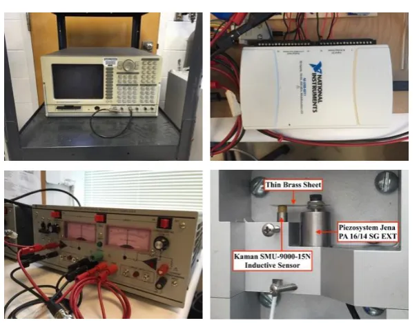
The experiment system consists of a piezo-based flexible structure where the displacement of the tip of the flexible beam was measured using an inductive sensor and all electrical signals were controlled using data acquisition (DAQ) as shown in Fig. 3.

Fig. 3. Experimental system diagram.

A flexible beam shown in Fig. 2 was made of a thin brass sheet with dimensions of 10 mm (width) by 25 mm (length) and 0.127 mm (thickness). As shown in Fig. 4 (bottom right), the one end of the flexible beam was attached to a piezo-actuator (Piezosystem Jena PA 16/14SC EXT) and the displacement of the other end was measured by an inductive sensor (Kaman SMU-9000-15N). A bi-polar power amplifier (Fig. 4, bottom left) was used to drive the piezo-actuator. The National Instruments NI USB-6211, see Fig. 4 (top right), was used to control electrical signals with its analog input and output channels.

4.2. System Model

The system G in Eq. (1) can be experimentally obtained by using the frequency response of the system, i.e., using the diagram given in Fig. 3

 

 

( ) 1

( )

( ) V ( ) ( )

o s o

a p i s a p i

V K V

y G

u K K V K K K V

 

 

  

 _ 

   _{ } 



  (10)

where  is frequency (rad/s), V is the pre-amplified input voltage ( V ), i V is the output voltage from o the inductive sensor ( V ), K_s 0.2012 μm/V is the inductive sensor gain, K_a  2 is the power amplifier gain, and Kp  1 is the piezo-actuator gain. For the experimental system, the input u is the voltage applied to the piezo-actuator in Volts ( V ) and the output y is the displacement of the tip of the flexible beam in microns ( μm ).

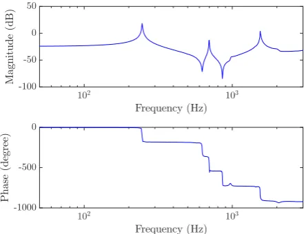
Frequency responses of the piezo-based flexible system obtained from a dynamic signal analyzer (SR785), see Fig. 4 (top left), by sending sine wave signals at different frequencies (between 50 and 2,500 Hz) to the system and measuring the displacement of the tip of the flexible beam with the inductive sensor are provided in Fig. 5. As shown in Fig. 5, example nonminimum-phase zeros are at a frequency of 600 Hz, approximately.

Fig. 5. Frequency response of the piezo-based flexible structure.

4.3. Desired Output Trajectory

A triangle trajectory, used in several scanning (such as AFM) operations [5], was used as the desired output-trajectory to illustrate the control approaches for the piezo-based flexible structure. One cycle data of the desired output-trajectory y are shown in Fig. 6 (top plot) and the complete (ten-cycle) data of the d i,

Fig. 6. Desired output-trajectory: (top) one-cycle data, (bottom left) ten-cycle data, and (bottom right) magnitude of the desired output-trajectory at different frequencies.

4.4. Results using Optimal Inversion-Based Control

While the simulation result obtained by using optimal inversion-based control shows reasonable output-tracking result, experimental output-output-tracking errors appear to be large, as shown in Fig. 9 (bottom left plot). Based on the frequency of the desired output-trajectory, values of r and q are chosen to be

2 50 ( )

2 50

w s s

  

 , ( ) 1000q s  w s( ),

1 ( )

( )

r s w s

 (11)

throughout this work. Magnitudes of the weighting matrices Q and R are shown in Fig. 7. The simulation result obtained using the optimal inversion-based control shows that the output y follows the desired sim trajectory y , Fig. 8 (bottom plot). The experimental output-tracking results from the optimal inversion-_d

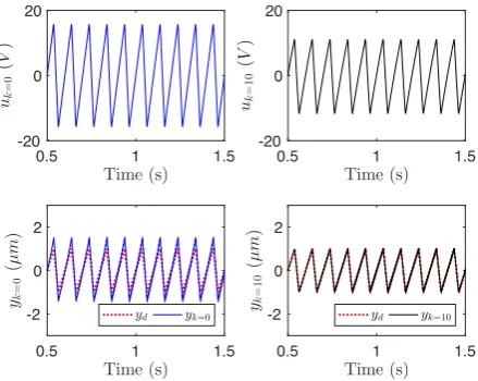
based control, i.e., zero iteration step (k0), are shown in Fig. 9 (left plots). The averaged data of seven trials of the output y were used to compute the output-tracking error e . Maximum output tracking error is

0.60 μm which is equal to 60% of the amplitude of the desired output-trajectory (1.5 μm ) as shown in Fig. 12 (bottom plot) and the output-tracking error e with zero iteration step (k0) is shown in Fig. 12 (top left plot).

Fig. 8. Simulation results using optimal inversion-based control: (top) input and (bottom) output.

Fig. 9. Experimental data with and without iterative inversion-based control: (left) results without iteration (k0), (right) results with iteration (k10), (top) input, and (bottom) output.

4.5. Results using Iterative-Based Optimal-Inverse Control

To decrease the output-tracking error e , iterative control was used with the appropriate iteration gain  based on criteria given in Eq. (8) and Eq. (9). The magnitude and phase analyses are shown in Fig. 10 (top and middle plots). As shown in Fig. 10 (bottom plot), the maximum allowable iteration gain  is two (2). Nevertheless, the iteration gain  used in the experiments was chosen to be

1, 2 200 ( )

0, otherwise,

 

    

 (12)

Fig. 10. Magnitude and phase difference between the system model (from frequency response data) and the optimal inverse model.

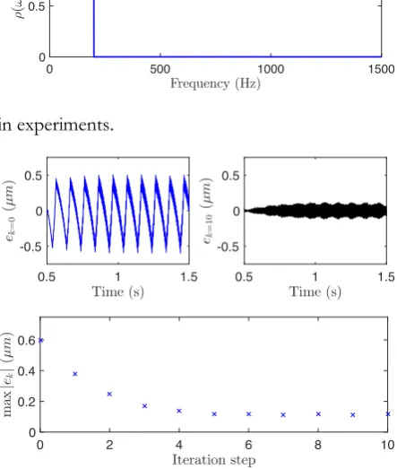
Fig. 11. Iteration gain used in experiments.

Fig. 12. Experimental output-tracking error: (top left) without iteration, (top right) with iteration, and (bottom) maximum output-tracking error at each iteration step.

5.

Conclusion

Acknowledgement

The author would like to thank Professor Santosh Devasia, the University of Washington, Seattle,

U.S.A., for invaluable guidance and Dr. Siriphan Manocheewa, Mahidol University, Thailand, for

useful suggestions. This work was supported by the National Science Foundation, U.S.A., under

Grant CMMI 1301452.

References

[1] A. Boekfah and S. Devasia, “Output-boundary regulation: High-speed AFM imaging

application,” in ASME Dynamic Systems and Control Conference, Palo Alto, CA, USA, 2013.

[2] G. M. Clayton, S. Tien, K. K. Leang, Q. Zou and S. Devasia, “A review of feedforward

control apporaches in nanopositioning for high speed SPM,” ASME Journal of Dyanmic Systems,

Measurement and Control, vol. 131, no. 6, pp. 1-19, 2009.

[3] S. Tien, Q. Zou, and S. Devasia, “Iterative control of dynamics-coupling-caused errors in

piezoscanners during high-speed AFM operation,” IEEE Transactions on Control Systems

Technology, vol. 13, no. 6, pp. 921 - 931, 2005.

[4] N. K. Gupta, “Frequency-shaped cost functionals - Extension of linear-quadratic-Gaussian

design methods,” Journal of Guidance, Control, and Dynamics, vol. 3, no. 6, pp. 529-535, 1980.

[5] K. S. Kim and Q. Zou, “A modeling-free inversion-based iterative feedforward control for

precision output tracking of linear time-invariant systems,” IEEE/ASME Transactions on