Learning Bayesian Networks Neapolitan R E pdf

(1)

Learning Bayesian Networks

Richard E. Neapolitan

Northeastern Illinois University

Chicago, Illinois

(2)

(3)

Preface

Bayesian networks are graphical structures for representing the probabilistic relationships among a large number of variables and doing probabilistic inference with those variables. During the 1980’s, a good deal of related research was done on developing Bayesian networks (belief networks, causal networks, influence diagrams), algorithms for performing inference with them, and applications that used them. However, the work was scattered throughout research articles. My purpose in writing the 1990 textProbabilistic Reasoning in Expert Systems was to unify this research and establish a textbook and reference for thefield which has come to be known as ‘Bayesian networks.’ The 1990’s saw the emergence of excellent algorithms for learning Bayesian networks from data. However, by 2000 there still seemed to be no accessible source for ‘learning Bayesian networks.’ Similar to my purpose a decade ago, the goal of this text is to provide such a source.

In order to make this text a complete introduction to Bayesian networks, I discuss methods for doing inference in Bayesian networks and influence di-agrams. However, there is no eﬀort to be exhaustive in this discussion. For example, I give the details of only two algorithms for exact inference with dis-crete variables, namely Pearl’s message passing algorithm and D’Ambrosio and Li’s symbolic probabilistic inference algorithm. It may seem odd that I present Pearl’s algorithm, since it is one of the oldest. I have two reasons for doing this: 1) Pearl’s algorithm corresponds to a model of human causal reasoning, which is discussed in this text; and 2) Pearl’s algorithm extends readily to an algorithm for doing inference with continuous variables, which is also discussed in this text.

The content of the text is as follows. Chapters 1 and 2 cover basics. Specifi-cally, Chapter 1 provides an introduction to Bayesian networks; and Chapter 2 discusses further relationships between DAGs and probability distributions such as d-separation, the faithfulness condition, and the minimality condition. Chap-ters 3-5 concern inference. Chapter 3 covers Pearl’s message-passing algorithm, D’Ambrosio and Li’s symbolic probabilistic inference, and the relationship of Pearl’s algorithm to human causal reasoning. Chapter 4 shows an algorithm for doing inference with continuous variable, an approximate inference algorithm, and finally an algorithm for abductive inference (finding the most probable explanation). Chapter 5 discusses influence diagrams, which are Bayesian net-works augmented with decision nodes and a value node, and dynamic Bayesian

(10)

networks and influence diagrams. Chapters 6-10 address learning. Chapters 6 and 7 concern parameter learning. Since the notation for these learning al-gorithm is somewhat arduous, I introduce the alal-gorithms by discussing binary variables in Chapter 6. I then generalize to multinomial variables in Chapter 7. Furthermore, in Chapter 7 I discuss learning parameters when the variables are continuous. Chapters 8, 9, and 10 concern structure learning. Chapter 8 shows the Bayesian method for learning structure in the cases of both discrete and continuous variables, while Chapter 9 discusses the constraint-based method for learning structure. Chapter 10 compares the Bayesian and constraint-based methods, and it presents several real-world examples of learning Bayesian net-works. The text ends by referencing applications of Bayesian networks in Chap-ter 11.

This is a text on learning Bayesian networks; it is not a text on artificial intelligence, expert systems, or decision analysis. However, since these arefields in which Bayesian networksfind application, they emerge frequently throughout the text. Indeed, I have used the manuscript for this text in my course on expert systems at Northeastern Illinois University. In one semester, I have found that I can cover the core of the following chapters: 1, 2, 3, 5, 6, 7, 8, and 9.

(11)

Part I

Basics

(12)

(13)

Chapter 1

Introduction to Bayesian

Networks

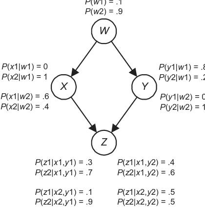
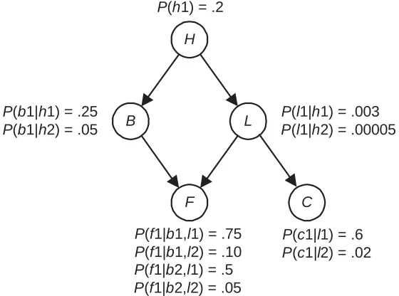
Consider the situation where one feature of an entity has a direct influence on another feature of that entity. For example, the presence or absence of a disease in a human being has a direct influence on whether a test for that disease turns out positive or negative. For decades, Bayes’ theorem has been used to perform probabilistic inference in this situation. In the current example, we would use that theorem to compute the conditional probability of an individual having a disease when a test for the disease came back positive. Consider next the situ-ation where several features are related through inference chains. For example, whether or not an individual has a history of smoking has a direct influence both on whether or not that individual has bronchitis and on whether or not that individual has lung cancer. In turn, the presence or absence of each of these diseases has a direct influence on whether or not the individual experiences fa-tigue. Also, the presence or absence of lung cancer has a direct influence on whether or not a chest X-ray is positive. In this situation, we would want to do probabilistic inference involving features that are not related via a direct influ-ence. We would want to determine, for example, the conditional probabilities both of bronchitis and of lung cancer when it is known an individual smokes, is fatigued, and has a positive chest X-ray. Yet bronchitis has no direct influence (indeed no influence at all) on whether a chest X-ray is positive. Therefore, these conditional probabilities cannot be computed using a simple application of Bayes’ theorem. There is a straightforward algorithm for computing them, but the probability values it requires are not ordinarily accessible; furthermore, the algorithm has exponential space and time complexity.

Bayesian networks were developed to address these diﬃculties. By exploiting conditional independencies entailed by influence chains, we are able to represent a large instance in a Bayesian network using little space, and we are often able to perform probabilistic inference among the features in an acceptable amount of time. In addition, the graphical nature of Bayesian networks gives us a much

(14)

H

B

F

L P(l1|h1) = .003 P(l1|h2) = .00005 P(b1|h1) = .25

P(b1|h2) = .05

P(h1) = .2

P(f1|b1,l1) = .75 P(f1|b1,l2) = .10 P(f1|b2,l1) = .5 P(f1|b2,l2) = .05

C

P(c1|l1) = .6 P(c1|l2) = .02

Figure 1.1: A Bayesian nework.

[image:14.612.193.474.125.333.2]

better intuitive grasp of the relationships among the features.

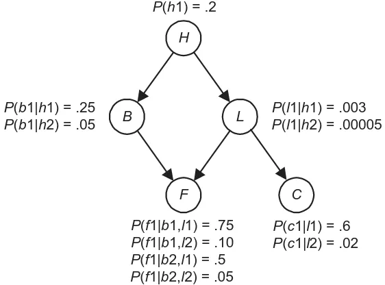
Figure 1.1 shows a Bayesian network representing the probabilistic relation-ships among the features just discussed. The values of the features in that network represent the following:

Feature Value When the Feature Takes this Value

H h1 There is a history of smoking

h2 There is no history of smoking

B b1 Bronchitis is present

b2 Bronchitis is absent

L l1 Lung cancer is present

l2 Lung cancer is absent

F f1 Fatigue is present

f2 Fatigue is absent

C c1 Chest X-ray is positive

c2 Chest X-ray is negative

(15)

1.1. BASICS OF PROBABILITY THEORY 5 edge fromH to C because a history of smoking has an influence on the result of a chest X-ray only through its influence on the presence of lung cancer. One way to construct Bayesian networks is by creating edges that represent direct influences as done here; however, there are other ways. Second, the probabilities in the network are the conditional probabilities of the values of each feature given every combination of values of the feature’s parents in the network, except in the case of roots they are prior probabilities. Third, probabilistic inference among the features can be accomplished using the Bayesian network. For example, we can compute the conditional probabilities both of bronchitis and of lung cancer when it is known an individual smokes, is fatigued, and has a positive chest X-ray. This Bayesian network is discussed again in Chapter 3 when we develop algorithms that do this inference.

The focus of this text is on learning Bayesian networks from data. For example, given we had values of the five features just discussed (smoking his-tory, bronchitis, lung cancer, fatigue, and chest X-ray) for a large number of individuals, the learning algorithms we develop might construct the Bayesian network in Figure 1.1. However, to make it a complete introduction to Bayesian networks, it does include a brief overview of methods for doing inference in Bayesian networks and using Bayesian networks to make decisions. Chapters 1 and 2 cover properties of Bayesian networks which we need in order to discuss both inference and learning. Chapters 3-5 concern methods for doing inference in Bayesian networks. Methods for learning Bayesian networks from data are discussed in Chapters 6-11. A number of successful experts systems (systems which make the judgements of an expert) have been developed which are based on Bayesian networks. Furthermore, Bayesian networks have been used to learn causal influences from data. Chapter 12 references some of these real-world ap-plications. To see the usefulness of Bayesian networks, you may wish to review that chapter before proceeding.

This chapter introduces Bayesian networks. Section 1.1 reviews basic con-cepts in probability. Next, Section 1.2 discusses Bayesian inference and illus-trates the classical way of using Bayes’ theorem when there are only two fea-tures. Section 1.3 shows the problem in representing large instances and intro-duces Bayesian networks as a solution to this problem. Finally, we discuss how Bayesian networks can often be constructed using causal edges.

1.1 Basics of Probability Theory

(16)

1.1.1 Probability Functions and Spaces

In 1933 A.N. Kolmogorov developed the set-theoretic definition of probability, which serves as a mathematical foundation for all applications of probability. We start by providing that definition.

Probability theory has to do with experiments that have a set of distinct outcomes. Examples of such experiments include drawing the top card from a deck of 52 cards with the 52 outcomes being the 52 diﬀerent faces of the cards; flipping a two-sided coin with the two outcomes being ‘heads’ and ‘tails’; picking a person from a population and determining whether the person is a smoker with the two outcomes being ‘smoker’ and ‘non-smoker’; picking a person from a population and determining whether the person has lung cancer with the two outcomes being ‘having lung cancer’ and ‘not having lung cancer’; after identifying 5 levels of serum calcium, picking a person from a population and determining the individual’s serum calcium level with the 5 outcomes being each of the 5 levels; picking a person from a population and determining the individual’s serum calcium level with the infinite number of outcomes being the continuum of possible calcium levels. The last two experiments illustrate two points. First, the experiment is not well-defined until we identify a set of outcomes. The same act (picking a person and measuring that person’s serum calcium level) can be associated with many diﬀerent experiments, depending on what we consider a distinct outcome. Second, the set of outcomes can be infinite. Once an experiment is well-defined, the collection of all outcomes is called the sample space. Mathematically, a sample space is a set and the outcomes are the elements of the set. To keep this review simple, we restrict ourselves tofinite sample spaces in what follows (You should consult a mathematical probability text such as [Ash, 1970] for a discussion of infinite sample spaces.). In the case of afinite sample space, every subset of the sample space is called anevent. A subset containing exactly one element is called anelementary event. Once a sample space is identified, a probability function is defined as follows:

Definition 1.1 Suppose we have a sample space Ω containing n distinct ele-ments. That is,

Ω=_{e1, e2, . . . en}.

A function that assigns a real number P(E) to each event E _⊆Ω is called a probability function on the set of subsets ofΩ if it satisfies the following conditions:

1. 0_≤P(_{ei})≤1 for1≤i≤n.

2. P(_{e1}) +P({e2}) +. . .+P({en}) = 1.

3. For each eventE=_{ei1, ei2, . . . eik}that is not an elementary event,

P(E) =P(_{ei1}) +P({ei2}) +. . .+P({eik}).

(17)

1.1. BASICS OF PROBABILITY THEORY 7 We often just sayP is a probability function onΩrather than saying on the set of subsets ofΩ.

Intuition for probability functions comes from considering games of chance as the following example illustrates.

Example 1.1 Let the experiment be drawing the top card from a deck of 52

cards. Then Ω contains the faces of the 52 cards, and using the principle of indiﬀerence, we assignP(_{e_}) = 1/52 for each e_∈Ω. Therefore, if we let kh and ks stand for the king of hearts and king of spades respectively,P(_{kh_}) = 1/52,P(_{ks_}) = 1/52, andP(_{kh, ks_}) =P(_{kh_}) +P(_{ks_}) = 1/26.

Theprinciple of indiﬀerence(a term popularized by J.M. Keynes in 1921) says elementary events are to be considered equiprobable if we have no reason to expect or prefer one over the other. According to this principle, when there are nelementary events the probability of each of them is the ratio 1/n. This is the way we often assign probabilities in games of chance, and a probability so assigned is called aratio.

The following example shows a probability that cannot be computed using the principle of indiﬀerence.

Example 1.2 Suppose we toss a thumbtack and consider as outcomes the two ways it could land. It could land on its head, which we will call ‘heads’, or it could land with the edge of the head and the end of the point touching the ground, which we will call ‘tails’. Due to the lack of symmetry in a thumbtack, we would not assign a probability of 1/2 to each of these events. So how can we compute the probability? This experiment can be repeated many times. In

1919Richard von Mises developed the relative frequency approach to probability which says that, if an experiment can be repeated many times, the probability of any one of the outcomes is the limit, as the number of trials approach infinity, of the ratio of the number of occurrences of that outcome to the total number of trials. For example, if mis the number of trials,

P(_{heads_}) = lim

m→∞

#heads

m .

So, if we tossed the thumbtack10,000times and it landed heads 3373times, we would estimate the probability of heads to be about .3373.

(18)

The next example illustrates a probability that cannot be obtained either with ratios or with relative frequencies.

Example 1.3 If you were going to bet on an upcoming basketball game between the Chicago Bulls and the Detroit Pistons, you would want to ascertain how probable it was that the Bulls would win. This probability is certainly not a ratio, and it is not a relative frequency because the game cannot be repeated many times under the exact same conditions (Actually, with your knowledge about the conditions the same.). Rather the probability only represents your belief concerning the Bulls chances of winning. Such a probability is called a

degree of belief or subjective probability. There are a number of ways

for ascertaining such probabilities. One of the most popular methods is the following, which was suggested by D. V. Lindley in1985. This method says an individual should liken the uncertain outcome to a game of chance by considering an urn containing white and black balls. The individual should determine for what fraction of white balls the individual would be indifferent between receiving a small prize if the uncertain outcome happened (or turned out to be true) and receiving the same small prize if a white ball was drawn from the urn. That fraction is the individual’s probability of the outcome. Such a probability can be constructed using binary cuts. If, for example, you were indifferent when the fraction was .75, for you P(_{bullswin_}) =.75. If I were indifferent when the fraction was .6, for me P(_{bullswin_}) =.6. Neither of us is right or wrong. Subjective probabilities are unlike ratios and relative frequencies in that they do not have objective values upon which we all must agree. Indeed, that is why they are called subjective.

Neapolitan [1996] discusses the construction of subjective probabilities fur-ther. In this text, byprobabilitywe ordinarily mean a degree of belief. When we are able to compute ratios or relative frequencies, the probabilities obtained agree with most individuals’ beliefs. For example, most individuals would assign a subjective probability of 1/13 to the top card being an ace because they would be indiﬀerent between receiving a small prize if it were the ace and receiving that same small prize if a white ball were drawn from an urn containing one white ball out of 13 total balls.

The following example shows a subjective probability more relevant to ap-plications of Bayesian networks.

(19)

1.1. BASICS OF PROBABILITY THEORY 9

patients with these exact same symptoms, to the actual relative frequency with which they have lung cancer.

It is straightforward to prove the following theorem concerning probability spaces.

Theorem 1.1 Let(Ω, P)be a probability space. Then 1. P(Ω) = 1.

2. 0_≤P(E)_≤1 for every E_⊆Ω.

3. For EandF_⊆Ω such thatE_∩F=_∅,

P(E_∪F) =P(E) +P(F).

Proof. The proof is left as an exercise.

The conditions in this theorem were labeled the axioms of probability theory by A.N. Kolmogorov in 1933. When Condition (3) is replaced by in-finitely countable additivity, these conditions are used to define a probability space in mathematical probability texts.

Example 1.5 Suppose we draw the top card from a deck of cards. Denote by

Queenthe set containing the4queens and byKingthe set containing the4kings. Then

P(Queen_∪King) =P(Queen) +P(King) = 1/13 + 1/13 = 2/13

because Queen_∩King = _∅. Next denote by Spade the set containing the 13

spades. The setsQueenandSpadeare not disjoint; so their probabilities are not additive. However, it is not hard to prove that, in general,

P(E_∪F) =P(E) +P(F)₋P(E_∩F).

So

P(Queen_∪Spade) = P(Queen) +P(Spade)₋P(Queen_∩Spade)

= 1 13+

1 4−

1 52=

4 13.

1.1.2 Conditional Probability and Independence

We have yet to discuss one of the most important concepts in probability theory, namely conditional probability. We do that next.

Definition 1.2 Let E and Fbe events such that P(F) ₆= 0. Then the condi-tional probability ofE givenF, denoted P(E_|F),is given by

P(E_|F) = P(E∩F)

(20)

The initial intuition for conditional probability comes from considering prob-abilities that are ratios. In the case of ratios, P(E_|F), as defined above, is the fraction of items inFthat are also inE. We show this as follows. Letnbe the number of items in the sample space,nF be the number of items inF, and nEF

be the number of items inE_∩F. Then

P(E_∩F)

P(F) =

nEF/n

nF/n

=nEF

nF

,

which is the fraction of items inFthat are also inE. As far as meaning,P(E_|F)

means the probability of Eoccurring given that we knowFhas occurred. Example 1.6 Again consider drawing the top card from a deck of cards, let

Queenbe the set of the4queens,RoyalCardbe the set of the12royal cards, and

Spadebe the set of the 13spades. Then

P(Queen) = 1 13

P(Queen_|RoyalCard) =P(Queen∩RoyalCard)

P(RoyalCard) = 1/13 3/13 =

1 3

P(Queen_|Spade) = P(Queen∩Spade)

P(Spade) = 1/52

1/4 = 1 13.

Notice in the previous example that P(Queen_|Spade) = P(Queen). This means thatfinding out the card is a spade does not make it more or less probable that it is a queen. That is, the knowledge of whether it is a spade is irrelevant to whether it is a queen. We say that the two events are independent in this case, which is formalized in the following definition.

Definition 1.3 Two events E and F are independent if one of the following hold:

1. P(E_|F) =P(E) and P(E)₆= 0,P(F)₆= 0. 2. P(E) = 0orP(F) = 0.

Notice that the definition states that the two events are independent even though it is based on the conditional probability of E given F. The reason is that independence is symmetric. That is, if P(E) ₆= 0 and P(F) ₆= 0, then

P(E_|F) =P(E)if and only ifP(F_|E) =P(F).It is straightforward to prove that EandFare independent if and only ifP(E_∩F) =P(E)P(F).

The following example illustrates an extension of the notion of independence. Example 1.7 Let E = _{kh, ks, qh_}, F = _{kh, kc, qh_}, G = _{kh, ks, kc, kd_}, wherekhmeans the king of hearts,ks means the king of spades, etc. Then

P(E) = 3 52

(21)

P(E_|G) = 2 4 =

1 2

P(E_|F_∩G) = 1 2.

SoEandFare not independent, but they are independent once we condition on

G.

In the previous example, Eand Fare said to be conditionally independent givenG. Conditional independence is very important in Bayesian networks and will be discussed much more in the sections that follow. Presently, we have the definition that follows and another example.

Definition 1.4 Two eventsEandFareconditionally independent givenG

if P(G)₆= 0 and one of the following holds:

1. P(E_|F_∩G) =P(E_|G) and P(E_|G)₆= 0,P(F_|G)₆= 0.

2. P(E_|G) = 0 orP(F_|G) = 0.

Another example of conditional independence follows.

Example 1.8 LetΩbe the set of all objects in Figure 1.2. Suppose we assign a probability of1/13to each object, and letBlackbe the set of all black objects,

Whitebe the set of all white objects,Square be the set of all square objects, and

One be the set of all objects containing a ‘1’. We then have

P(One) = 5 13

P(One_|Square) = 3 8

P(One_|Black) = 3 9=

1 3

P(One_|Square_∩Black) = 2 6=

1 3

P(One_|White) = 2 4 =

1 2

P(One_|Square_∩White) = 1 2.

SoOne andSquare are not independent, but they are conditionally independent givenBlackand given White.

(22)

1

2

1

2

1

2

Figure 1.2: Containing a ‘1’ and being a square are not independent, but they are conditionally independent given the object is black and given it is white.

E1∪E2 ∪. . .∪En = Ω. Such events are called mutually exclusive and exhaustive. Then thelaw of total probability says for any other eventF,

P(F) =

n X

i=1

P(F_∩Ei). (1.1)

IfP(Ei)6= 0, then P(F∩Ei) =P(F|Ei)P(Ei). Therefore, ifP(Ei)6= 0for alli, the law is often applied in the following form:

P(F) =

n X

i=1

P(F_|Ei)P(Ei). (1.2)

It is straightforward to derive both the axioms of probability theory and the rule for conditional probability when probabilities are ratios. However, they can also be derived in the relative frequency and subjectivistic frameworks (See [Neapolitan, 1990].). These derivations make the use of probability theory compelling for handling uncertainty.

1.1.3 Bayes’ Theorem

For decades conditional probabilities of events of interest have been computed from known probabilities using Bayes’ theorem. We develop that theorem next. Theorem 1.2 (Bayes) Given two events E and F such that P(E) ₆= 0 and P(F)₆= 0, we have

P(E_|F) = P(F|E)P(E)

P(F) . (1.3)

Furthermore, givennmutually exclusive and exhaustive eventsE1,E2, . . .En

such that P(Ei)6= 0for all i, we have for1≤i≤n,

P(Ei|F) =

P(F_|Ei)P(Ei)

(23)

Proof. To obtain Equality 1.3, wefirst use the definition of conditional proba-bility as follows:

P(E_|F) = P(E∩F)

P(F) and P(F|E) =

P(F_∩E)

P(E) .

Next we multiply each of these equalities by the denominator on its right side to show that

P(E_|F)P(F) =P(F_|E)P(E)

because they both equal P(E_∩F). Finally, we divide this last equality byP(F)

to obtain our result.

To obtain Equality 1.4, we place the expression forF, obtained using the rule of total probability (Equality 1.2), in the denominator of Equality 1.3.

Both of the formulas in the preceding theorem are calledBayes’ theorem because they were originally developed by Thomas Bayes (published in 1763). Thefirst enables us to computeP(E_|F)if we knowP(F_|E),P(E), andP(F), while the second enables us to compute P(Ei|F)if we know P(F|Ej) and P(Ej) for

1_≤j_≤n. Computing a conditional probability using either of these formulas is calledBayesian inference. An example of Bayesian inference follows: Example 1.9 Let Ω be the set of all objects in Figure 1.2, and assign each object a probability of1/13. LetOnebe the set of all objects containing a1,Two

be the set of all objects containing a 2, andBlackbe the set of all black objects. Then according to Bayes’ Theorem,

P(One_|Black) = P(Black|One)P(One)

P(Black_|One)P(One) +P(Black_|Two)P(Two)

= (

3 5)(

5 13)

(3₅)(₁₃5) + (6₈)(₁₃8) = 1 3,

which is the same value we get by computingP(One_|Black)directly.

The previous example is not a very exciting application of Bayes’ Theorem as we can just as easily compute P(One_|Black) directly. Section 1.2 discusses useful applications of Bayes’ Theorem.

1.1.4 Random Variables and Joint Probability

Distribu-tions

We have onefinal concept to discuss in this overview, namely that of a random variable. The definition shown here is based on the set-theoretic definition of probability given in Section 1.1.1. In Section 1.2.2 we provide an alternative definition which is more pertinent to the way random variables are used in practice.

(24)

That is, a random variable assigns a unique value to each element (outcome) in the sample space. The set of values random variableXcan assume is called thespaceof X. A random variable is said to be discreteif its space isfinite or countable. In general, we develop our theory assuming the random variables are discrete. Examples follow.

Example 1.10 Let Ω contain all outcomes of a throw of a pair of six-sided dice, and let P assign 1/36 to each outcome. Then Ω is the following set of ordered pairs:

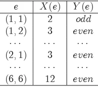
[image:24.612.282.379.310.399.2]

Ω=_{(1,1),(1,2),(1,3),(1,4),(1,5),(1,6),(2,1),(2,2), . . .(6,5),(6,6)_}. Let the random variableXassign the sum of each ordered pair to that pair, and let the random variable Y assign ‘odd’ to each pair of odd numbers and ‘even’ to a pair if at least one number in that pair is an even number. The following table shows some of the values ofX andY:

e X(e) Y(e) (1,1) 2 odd

(1,2) 3 even

· · · ·

(2,1) 3 even

· · · ·

(6,6) 12 even

The space ofXis_{2,3,4,5,6,7,8,9,10,11,12_}, and that ofY is_{odd, even_}.

For a random variable X, we use X =x to denote the set of all elements

e_∈ΩthatX maps to the value ofx. That is,

X=x represents the event _{esuch that X(e) =x_}.

Note the diﬀerence betweenXandx. Smallxdenotes any element in the space ofX, while X is a function.

Example 1.11 LetΩ,P, andX be as in Example 1.10. Then X= 3 represents the event _{(1,2),(2,1)_}and

P(X= 3) = 1 18.

It is not hard to see that a random variable induces a probability function on its space. That is, if we define PX({x}) ≡ P(X = x), then PX is such a probability function.

Example 1.12 Let Ω contain all outcomes of a throw of a single die, let P assign 1/6to each outcome, and let Z assign ‘even’ to each even number and ‘odd’ to each odd number. Then

PZ({even}) =P(Z =even) =P({2,4,6}) =

(25)

PZ({odd}) =P(Z=odd) =P({1,3,5}) =

1 2.

We rarely refer toPX({x}). Rather we only reference the original probability functionP, and we callP(X=x)theprobability distributionof the random variable X. For brevity, we often just say ‘distribution’ instead of ‘probability distribution’. Furthermore, we often use xalone to represent the event X=x, and so we writeP(x)instead ofP(X=x). We refer toP(x)as ‘the probability of x’.

LetΩ,P, andX be as in Example 1.10. Then ifx= 3,

P(x) =P(X=x) = 1 18.

Given two random variablesXandY, defined on the same sample spaceΩ,

we use X=x, Y =y to denote the set of all elementse_∈Ωthat are mapped both byX toxand byY to y. That is,

X=x, Y =y represents the event

{esuch thatX(e) =x_}_∩_{esuch thatY(e) =y_}.

Example 1.13 LetΩ,P,X, andY be as in Example 1.10. Then X= 4, Y =odd represents the event _{(1,3),(3,1)_}, and

P(X= 4, Y =odd) = 1/18.

Clearly, two random variables induce a probability function on the Cartesian product of their spaces. As is the case for a single random variable, we rarely refer to this probability function. Rather we reference the original probability function. That is, we refer to P(X = x, Y = y), and we call this thejoint probability distribution of X and Y. IfA =_{X, Y_}, we also call this the joint probability distribution of A. Furthermore, we often just say ‘joint distribution’ or ‘probability distribution’.

For brevity, we often use x, y to represent the event X = x, Y = y, and so we write P(x, y) instead of P(X = x, Y = y). This concept extends in a straightforward way to three or more random variables. For example, P(X =

x, Y =y, Z =z) is the joint probability distribution function of the variables

X,Y, andZ, and we often writeP(x, y, z).

Example 1.14 LetΩ,P,X, andY be as in Example 1.10. Then ifx= 4and y=odd,

P(x, y) =P(X=x, Y =y) = 1/18.

If, for example, we letA=_{X, Y_}anda=_{x, y_}, we use A=a to represent X=x, Y =y,

and we often write P(a) instead of P(A = a). The same notation extends to the representation of three or more random variables. For consistency, we set

(26)

Example 1.15 Let Ω, P, X, and Y be as in Example 1.10. If A = _{X, Y_},

a=_{x, y_},x= 4, andy=odd,

P(A=a) =P(X=x, Y =y) = 1/18.

This notation entails that if we have, for example, two sets of random vari-ablesA=_{X, Y_}andB=_{Z, W_}, then

A=a,B=b represents X=x, Y =y, Z=z, W =w.

Given a joint probability distribution, the law of total probability (Equality 1.1) implies the probability distribution of any one of the random variables can be obtained by summing over all values of the other variables. It is left as an exercise to show this. For example, suppose we have a joint probability distributionP(X=x, Y =y). Then

P(X=x) =X

y

P(X=x, Y =y),

where P_y means the sum as y goes through all values of Y. The probability distributionP(X=x)is called themarginal probability distributionofX

because it is obtained using a process similar to adding across a row or column in a table of numbers. This concept also extends in a straightforward way to three or more random variables. For example, if we have a joint distributionP(X=

x, Y =y, Z=z)ofX,Y, andZ, the marginal distributionP(X=x, Y =y)of

X andY is obtained by summing over all values ofZ. IfA=_{X, Y_}, we also call this themarginal probability distributionofA.

Example 1.16 LetΩ,P,X, andY be as in Example 1.10. Then

P(X= 4) = X

y

P(X= 4, Y =y)

= P(X= 4, Y =odd) +P(X= 4, Y =even) = 1 18+

1 36 =

1 12.

The following example reviews the concepts covered so far concerning ran-dom variables:

(27)

1.1. BASICS OF PROBABILITY THEORY 17 Case Sex Height(inches) Wage($)

1 female 64 30,000

2 female 64 30,000

3 female 64 40,000

4 female 64 40,000

5 female 68 30,000

6 female 68 40,000

7 male 64 40,000 8 male 64 50,000 9 male 68 40,000 10 male 68 50,000 11 male 70 40,000 12 male 70 50,000

Let the random variables S, H andW respectively assign the sex, height and wage of an individual to that individual. Then the distributions of the three variables are as follows (Recall that, for example,P(s)representsP(S=s).):

s P(s)

female 1/2

male 1/2

h P(h) 64 1/2 68 1/3 70 1/6

w P(w) 30,000 1/4 40,000 1/2 50,000 1/4

The joint distribution of S andH is as follows:

s h P(s, h)

female 64 1/3

female 68 1/6

female 70 0

male 64 1/6

male 68 1/6

male 70 1/6

The following table also shows the joint distribution of S andH and illustrates that the individual distributions can be obtained by summing the joint distribu-tion over all values of the other variable:

h 64 68 70 Distribution of S s

female 1/3 1/6 0 1/2

male 1/6 1/6 1/6 1/2

Distribution of H 1/2 1/3 1/6

(28)

s h w P(s, h, w)

female 64 30,000 1/6

female 64 40,000 1/6

female 64 50,000 0

female 68 30,000 1/12

· · · ·

We have the following definition:

Definition 1.6 Suppose we have a probability space(Ω, P), and two setsAand

Bcontaining random variables defined onΩ. Then the setsAandBare said to beindependentif, for all values of the variables in the setsaandb, the events

A=aandB=bare independent. That is, eitherP(a) = 0or P(b) = 0or

P(a_|b) =P(a).

When this is the case, we write

IP(A,B),

whereIP stands for independent inP.

Example 1.18 Let Ω be the set of all cards in an ordinary deck, and let P assign1/52to each card. Define random variables as follows:

Variable Value Outcomes Mapped to this Value

R r1 All royal cards

r2 All nonroyal cards

T t1 All tens and jacks

t2 All cards that are neither tens nor jacks

S s1 All spades

s2 All nonspades

Then we maintain the sets_{R, T_}and_{S_}are independent. That is,

IP({R, T},{S}).

To show this, we need show for all values ofr,t, andsthat

P(r, t_|s) =P(r, t).

(29)

s r t P(r, t_|s) P(r, t)

s1 r1 t1 1/13 4/52 = 1/13

s1 r1 t2 2/13 8/52 = 2/13

s1 r2 t1 1/13 4/52 = 1/13

s1 r2 t2 9/13 36/52 = 9/13

s2 r1 t1 3/39 = 1/13 4/52 = 1/13

s2 r1 t2 6/39 = 2/13 8/52 = 2/13

s2 r2 t1 3/39 = 1/13 4/52 = 1/13

s2 r2 t2 27/39 = 9/13 36/52 = 9/13

Definition 1.7 Suppose we have a probability space (Ω, P), and three sets A,

B, andCcontaining random variable defined onΩ. Then the setsAandB are said to be conditionally independent given the set Cif, for all values of the variables in the sets a, b,and c, whenever P(c)₆= 0, the events A=a and

B = b are conditionally independent given the event C = c. That is, either P(a_|c) = 0orP(b_|c) = 0 or

P(a_|b,c) =P(a_|c).

When this is the case, we write

IP(A,B|C).

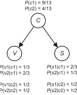
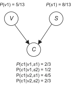
Example 1.19 Let Ωbe the set of all objects in Figure 1.2, and let P assign

1/13to each object. Define random variablesS (for shape),V (for value), and C (for color) as follows:

Variable Value Outcomes Mapped to this Value

V v1 All objects containing a ‘1’ v2 All objects containing a ‘2’

S s1 All square objects

s2 All round objects

C c1 All black objects

c2 All white objects

Then we maintain that _{V_}and_{S_}are conditionally independent given _{C_}. That is,

IP({V},{S}|{C}).

To show this, we need show for all values ofv,s, andcthat

P(v_|s, c) =P(v_|c).

The results in Example 1.8 show P(v1_|s1, c1) = P(v1_|c1) and P(v1_|s1, c2) =

(30)

c s v P(v_|s, c) P(v_|c)

c1 s1 v1 2/6 = 1/3 3/9 = 1/3

c1 s1 v2 4/6 = 2/3 6/9 = 2/3

c1 s2 v1 1/3 3/9 = 1/3

c1 s2 v2 2/3 6/9 = 2/3

c2 s1 v1 1/2 2/4 = 1/2

c2 s1 v2 1/2 2/4 = 1/2

c2 s2 v1 1/2 2/4 = 1/2

c2 s2 v2 1/2 2/4 = 1/2

For the sake of brevity, we sometimes only say ‘independent’ rather than ‘conditionally independent’. Furthermore, when a set contains only one item, we often drop the set notation and terminology. For example, in the preceding example, we might sayV andSare independent givenC and writeIP(V, S|C). Finally, we have thechain rulefor random variables, which says that given

nrandom variablesX1, X2, . . . Xn, defined on the same sample spaceΩ,

P(x1, x2, . . .xn) =P(xn|xn−1, xn−2, . . .x1)· · ·P(x2|x1)P(x1)

wheneverP(x1, x2, . . .xn)6= 0. It is straightforward to prove this rule using the rule for conditional probability.

1.2 Bayesian Inference

We use Bayes’ Theorem when we are not able to determine the conditional probability of interest directly, but we are able to determine the probabilities on the right in Equality 1.3. You may wonder why we wouldn’t be able to compute the conditional probability of interest directly from the sample space. The reason is that in these applications the probability space is not usually developed in the order outlined in Section 1.1. That is, we do not identify a sample space, determine probabilities of elementary events, determine random variables, and then compute values in joint probability distributions. Instead, we identify random variables directly, and we determine probabilistic relationships among the random variables. The conditional probabilities of interest are often not the ones we are able to judge directly. We discuss next the meaning of random variables and probabilities in Bayesian applications and how they are identified directly. After that, we show how a joint probability distribution can be determined withoutfirst specifying a sample space. Finally, we show a useful application of Bayes’ Theorem.

1.2.1 Random Variables and Probabilities in Bayesian

Ap-plications

(31)

1.2. BAYESIAN INFERENCE 21 Bayesian inference. In this subsection and the next we develop an alternative definition that does.

When doing Bayesian inference, there is some entity which has features, the states of which we wish to determine, but which we cannot determine for certain. So we settle for determining how likely it is that a particular feature is in a particular state. The entity might be a single system or a set of systems. An example of a single system is the introduction of an economically beneficial chemical which might be carcinogenic. We would want to determine the relative risk of the chemical versus its benefits. An example of a set of entities is a set of patients with similar diseases and symptoms. In this case, we would want to diagnose diseases based on symptoms.

In these applications, a random variable represents some feature of the entity being modeled, and we are uncertain as to the values of this feature for the particular entity. So we develop probabilistic relationships among the variables. When there is a set of entities, we assume the entities in the set all have the same probabilistic relationships concerning the variables used in the model. When this is not the case, our Bayesian analysis is not applicable. In the case of the chemical introduction, features may include the amount of human exposure and the carcinogenic potential. If these are our features of interest, we identify the random variablesHumanExposureandCarcinogenicP otential(For simplicity, our illustrations include only a few variables. An actual application ordinarily includes many more than this.). In the case of a set of patients, features of interest might include whether or not a disease such as lung cancer is present, whether or not manifestations of diseases such as a chest X-ray are present, and whether or not causes of diseases such as smoking are present. Given these features, we would identify the random variables ChestXray, LungCancer, andSmokingHistory. After identifying the random variables, we distinguish a set of mutually exclusive and exhaustive values for each of them. The possible values of a random variable are the diﬀerent states that the feature can take. For example, the state ofLungCancer could bepresentorabsent, the state of

ChestXray could be positive or negative, and the state of SmokingHistory

could be yes or no. For simplicity, we have only distinguished two possible values for each of these random variables. However, in general they could have any number of possible values or they could even be continuous. For example, we might distinguish 5 diﬀerent levels of smoking history (one pack or more for at least 10 years, two packs or more for at least 10 years, three packs or more for at lest ten years, etc.). The specification of the random variables and their values not only must be precise enough to satisfy the requirements of the particular situation being modeled, but it also must be suﬃciently precise to pass the clarity test, which was developed by Howard in 1988. That test is as follows: Imagine a clairvoyant who knows precisely the current state of the world (or future state if the model concerns events in the future). Would the clairvoyant be able to determine unequivocally the value of the random variable? For example, in the case of the chemical introduction, if we give

(32)

when the average (over all individuals), of the individual daily average skin contact, exceeds 6 grams of material, the clarity test is passed because the clairvoyant can answer precisely whether the contact exceeds that. In the case of a medical application, if we giveSmokingHistory only the values yes and

no, the clarity test is not passed because we do not know whether yes means smoking cigarettes, cigars, or something else, and we have not specified how long smoking must have occurred for the value to beyes. On the other hand, if we sayyesmeans the patient has smoked one or more packs of cigarettes every day during the past 10 years, the clarity test is passed.

After distinguishing the possible values of the random variables (i.e. their spaces), we judge the probabilities of the random variables having their values. However, in general we do not always determine prior probabilities; nor do we de-termine values in a joint probability distribution of the random variables. Rather we ascertain probabilities, concerning relationships among random variables, that are accessible to us. For example, we might determine the prior probability

P(LungCancer=present), and the conditional probabilities P(ChestXray=

positive_|LungCancer = present), P(ChestXray = positive_|LungCancer =

absent), P(LungCancer = present_| SmokingHistory = yes), and finally

P(LungCancer = present_|SmokingHistory = no). We would obtain these probabilities either from a physician or from data or from both. Thinking in terms of relative frequencies, P(LungCancer = present_|SmokingHistory =

yes)can be estimated by observing individuals with a smoking history, and de-termining what fraction of these have lung cancer. A physician is used to judging such a probability by observing patients with a smoking history. On the other hand, one does not readily judge values in a joint probability distribution such as

P(LungCancer=present, ChestXray=positive, SmokingHistory =yes). If this is not apparent, just think of the situation in which there are 100 or more random variables (which there are in some applications) in the joint probability distribution. We can obtain data and think in terms of probabilistic relation-ships among a few random variables at a time; we do not identify the joint probabilities of several events.

As to the nature of these probabilities, considerfirst the introduction of the toxic chemical. The probabilities of the values ofCarcinogenicP otential will be based on data involving this chemical and similar ones. However, this is certainly not a repeatable experiment like a coin toss, and therefore the prob-abilities are not relative frequencies. They are subjective probprob-abilities based on a careful analysis of the situation. As to the medical application involv-ing a set of entities, we often obtain the probabilities from estimates of rel-ative frequencies involving entities in the set. For example, we might obtain

(33)

1.2. BAYESIAN INFERENCE 23 feel that we are splitting hairs. Namely, you may argue the following: “This subjective probability regarding a specific patient is obtained from a relative frequency and therefore has the same value as it. We are simply calling it a subjective probability rather than a relative frequency.” But even this is not the case. Even if the probabilities used to do Bayesian inference are obtained from frequency data, they are only estimates of the actual relative frequencies. So they are subjective probabilities obtained from estimates of relative frequen-cies; they are not relative frequencies. When we manipulate them using Bayes’ theorem, the resultant probability is therefore also only a subjective probability. Once we judge the probabilities for a given application, we can often ob-tain values in a joint probability distribution of the random variables. Theo-rem 1.5 in Section 1.3.3 obtains a way to do this when there are many vari-ables. Presently, we illustrate the case of two variables. Suppose we only identify the random variables LungCancerandChestXray, and we judge the prior probability P(LungCancer = present), and the conditional probabili-ties P(ChestXray = positive_|LungCancer =present)and P(ChestXray =

positive_|LungCancer =absent). Probabilities of values in a joint probability distribution can be obtained from these probabilities using the rule for condi-tional probability as follows:

P(present, positive) =P(positive_|present)P(present)

P(present, negative) =P(negative_|present)P(present)

P(absent, positive) =P(positive_|absent)P(absent)

P(absent, negative) =P(negative_|absent)P(absent).

Note that we used our abbreviated notation. We see then that at the outset we identify random variables and their probabilistic relationships, and values in a joint probability distribution can then often be obtained from the probabilities relating the random variables. So what is the sample space? We can think of the sample space as simply being the Cartesian product of the sets of all possible values of the random variables. For example, consider again the case where we only identify the random variablesLungCancerandChestXray, and ascertain probability values in a joint distribution as illustrated above. We can define the following sample space:

Ω=

{(present, positive),(present, negative),(absent, positive),(absent, negative)_}.

We can consider each random variable a function on this space that maps each tuple into the value of the random variable in the tuple. For example,

LungCancer would map(present, positive)and (present, negative) each into

present.We then assign each elementary event the probability of its correspond-ing event in the joint distribution. For example, we assign

ˆ

(34)

It is not hard to show that this does yield a probability function onΩ and that the initially assessed prior probabilities and conditional probabilities are the probabilities they notationally represent in this probability space (This is a special case of Theorem 1.5.).

Since random variables are actually identified first and only implicitly be-come functions on an implicit sample space, it seems we could develop the con-cept of a joint probability distribution without the explicit notion of a sample space. Indeed, we do this next. Following this development, we give a theorem showing that any such joint probability distribution is a joint probability dis-tribution of the random variables with the variables considered as functions on an implicit sample space. Definition 1.1 (of a probability function) and Defi-nition 1.5 (of a random variable) can therefore be considered the fundamental definitions for probability theory because they pertains both to applications where sample spaces are directly identified and ones where random variables are directly identified.

1.2.2 A Definition of Random Variables and Joint

Proba-bility Distributions for Bayesian Inference

For the purpose of modeling the types of problems discussed in the previous subsection, we can define arandom variableXas a symbol representing any one of a set of values, called the space of X. For simplicity, we will assume the space ofXis countable, but the theory extends naturally to the case where it is not. For example, we could identify the random variableLungCancer as having the space_{present, absent_}. We use the notationX=xas a primitive which is used in probability expressions. That is,X=xis not defined in terms of anything else. For example, in applicationLungCancer=presentmeans the entity being modeled has lung cancer, but mathematically it is simply a primi-tive which is used in probability expressions. Given this definition and primiprimi-tive, we have the following direct definition of a joint probability distribution: Definition 1.8 Let a set ofnrandom variablesV=_{X1, X2, . . . Xn}be

speci-fied such that eachXi has a countably infinite space. A function, that assigns a

real number P(X1 =x1, X2 =x2, . . . Xn =xn)to every combination of values

of thexi’s such that the value of xi is chosen from the space ofXi, is called a

joint probability distribution of the random variables inV if it satisfies the following conditions:

1. For every combination of values of thexi’s,

0_≤P(X1=x1, X2=x2, . . . Xn=xn)≤1.

2. We have

X

x1,x2,...xn

(35)

1.2. BAYESIAN INFERENCE 25

The notation P_x1,x2_,..._x_n means the sum as the variables x1, . . . xn go

through all possible values in their corresponding spaces.

Note that a joint probability distribution, obtained by defining random vari-ables as functions on a sample space, is one way to create a joint probability distribution that satisfies this definition. However, there are other ways as the following example illustrates:

Example 1.20 LetV=_{X, Y_}, letXandY have spaces_{x1, x2_}1_and_{_y₁_{, y}₂_}

respectively, and let the following values be specified:

P(X=x1) =.2 P(Y =y1) =.3

P(X=x2) =.8 P(Y =y2) =.7.

Next define a joint probability distribution of X andY as follows:

P(X=x1, Y =y1) =P(X=x1)P(Y =y1) = (.2)(.3) =.06

P(X=x1, Y =y2) =P(X=x1)P(Y =y2) = (.2)(.7) =.14

P(X=x2, Y =y1) =P(X=x2)P(Y =y1) = (.8)(.3) =.24

P(X=x2, Y =y2) =P(X=x2)P(Y =y2) = (.8)(.7) =.56.

Since the values sum to1, this is another way of specifying a joint probability distribution according to Definition 1.8. This is how we would specify the joint distribution if we feltX andY were independent.

Notice that our original specifications, P(X = xi) and P(Y = yi), nota-tionally look like marginal distributions of the joint distribution developed in Example 1.20. However, Definition 1.8 only defines a joint probability distri-butionP; it does not mention anything about marginal distributions. So the initially specified values do not represent marginal distributions of our joint dis-tribution P according to that definition alone. The following theorem enables us to consider them marginal distributions in the classical sense, and therefore justifies our notation.

Theorem 1.3 Let a set of random variablesV be given and let a joint proba-bility distribution of the variables in V be specified according to Definition 1.8. LetΩ be the Cartesian product of the sets of all possible values of the random variables. Assign probabilities to elementary events in Ωas follows:

ˆ

P(_{(x1, x2, . . . xn)}) =P(X1=x1, X2=x2, . . . Xn =xn).

These assignments result in a probability function onΩaccording to Definition 1.1. Furthermore, if we let Xˆi denote a function (random variable in the

clas-sical sense) on this sample space that maps each tuple inΩto the value ofxi in

1_{We use subscripted variables} _X

i to denote diﬀerent random variables. So we do not

(36)

that tuple, then the joint probability distribution of the Xˆi’s is the same as the

originally specified joint probability distribution.

Proof. The proof is left as an exercise.

Example 1.21 Suppose we directly specify a joint probability distribution ofX andY, each with space _{x1, x2_}and _{y1, y2_}respectively, as done in Example 1.20. That is, we specify the following probabilities:

P(X=x1, Y =y1)

P(X=x1, Y =y2)

P(X=x2, Y =y1)

P(X=x2, Y =y2).

Next we letΩ=_{(x1, y1),(x1, y2),(x2, y1),(x2, y2)_}, and we assign

ˆ

P(_{(xi, yj)_}) =P(X=xi, Y =yj).

Then we letXˆ andYˆ be functions on Ωdefined by the following tables:

x y Xˆ((x, y))

x1 y1 x1

x1 y2 x1

x2 y1 x2

x2 y2 x2

x y Yˆ((x, y))

x1 y1 y1

x1 y2 y2

x2 y1 y1

x2 y2 y2

Theorem 1.3 says the joint probability distribution of these random variables is the same as the originally specified joint probability distribution. Let’s illustrate this:

ˆ

P( ˆX=x1,Yˆ =y1) = Pˆ(_{(x1, y1),(x1, y2)_}_∩_{(x1, y1),(x2, y1)_}) = Pˆ(_{(x1, y1)_})

= P(X=x1, Y =y1).

Due to Theorem 1.3, we need no postulates for probabilities of combinations of primitives not addressed by Definition 1.8. Furthermore, we need no new definition of conditional probability for joint distributions created according to that definition. We can just postulate that both obtain values according to the set theoretic definition of a random variable. For example, consider Example 1.20. Due to Theorem 1.3,Pˆ( ˆX=x1)is simply a value in a marginal distribution of the joint probability distribution. So its value is computed as follows:

ˆ

P( ˆX=x1) = Pˆ( ˆX=x1,Yˆ =y1) + ˆP( ˆX=x1,Yˆ =y2) = P(X=x1, Y =y1) +P(X=x1, Y =y2) = P(X=x1)P(Y =y1) +P(X=x1)P(Y =y2) = P(X=x1)[P(Y =y1) +P(Y =y2)]

(37)

1.2. BAYESIAN INFERENCE 27 which is the originally specified value. This result is a special case of Theorem 1.5.

Note that the specified probability values are not by necessity equal to the probabilities they notationally represent in the marginal probability distribu-tion. However, since we used the rule for independence to derive the joint probability distribution from them, they are in fact equal to those values. For example, if we had definedP(X=x1, Y =y1) = P(X =x2)P(Y =y1), this would not be the case. Of course we would not do this. In practice, all specified values are always the probabilities they notationally represent in the resultant probability space (Ω,Pˆ). Since this is the case, we will no longer show carats overP orXwhen referring to the probability function in this space or a random variable on the space.

Example 1.22 LetV=_{X, Y_}, letXandY have spaces_{x1, x2_}and_{y1, y2_}

respectively, and let the following values be specified:

P(X=x1) =.2 P(Y =y1_|X=x1) =.3

P(X=x2) =.8 P(Y =y2_|X=x1) =.7

P(Y =y1_|X=x2) =.4

P(Y =y2_|X=x2) =.6.

Next define a joint probability distribution of X andY as follows:

P(X=x1, Y =y1) =P(Y =y1_|X=x1)P(X=x1) = (.3)(.2) =.06

P(X=x1, Y =y2) =P(Y =y2_|X=x1)P(X=x1) = (.7)(.2) =.14

P(X=x2, Y =y1) =P(Y =y1_|X=x2)P(X=x2) = (.4)(.8) =.32

P(X=x2, Y =y2) =P(Y =y2_|X=x2)P(X=x2) = (.6)(.8) =.48. Since the values sum to1, this is another way of specifying a joint probability distribution according to Definition 1.8. As we shall see in Example 1.23 in the following subsection, this is the way they are specified in simple applications of Bayes’ Theorem.

In the remainder of this text, we will create joint probability distributions using Definition 1.8. Before closing, we note that this definition pertains to any application in which we model naturally occurring phenomena by identifying random variables directly, which includes most applications of statistics.

1.2.3 A Classical Example of Bayesian Inference

(38)

Example 1.23 Suppose Joe has a routine diagnostic chest X-ray required of all new employees at Colonial Bank, and the X-ray comes back positive for lung cancer. Joe then becomes certain he has lung cancer and panics. But should he? Without knowing the accuracy of the test, Joe really has no way of knowing how probable it is that he has lung cancer. When he discovers the test is not absolutely conclusive, he decides to investigate its accuracy and he learns that it has a false negative rate of.4and a false positive rate of.02. We represent this accuracy as follows. First we define these random variables:

Variable Value When the Variable Takes This Value

T est positive X-ray is positive negative X-ray is negative LungCancer present Lung cancer is present

absent Lung cancer is absent

We then have these conditional probabilities:

P(T est=positive_|LungCancer=present) =.6

P(T est=positive_|LungCancer=absent) =.02.

Given these probabilities, Joe feels a little better. However, he then realizes he still does not know how probable it is that he has lung cancer. That is, the prob-ability of Joe having lung cancer isP(LungCancer=present_|T est=positive), and this is not one of the probabilities listed above. Joe finally recalls Bayes’ theorem and realizes he needs yet another probability to determine the probability of his having lung cancer. That probability isP(LungCancer=present),which is the probability of his having lung cancer before any information on the test results were obtained. Even though this probability is not based on any informa-tion concerning the test results, it is based on some informainforma-tion. Specifically, it is based on all information (relevant to lung cancer) known about Joe before he took the test. The only information about Joe, before he took the test, was that he was one of a class of employees who took the test routinely required of new employees. So, when he learns only1out of every1000new employees has lung cancer, he assigns.001toP(LungCancer=present). He then employs Bayes’ theorem as follows (Note that we again use our abbreviated notation):

P(present_|positive)

= P(positive|present)P(present)

P(positive_|present)P(present) +P(positive_|absent)P(absent)

= (.6)(.001) (.6)(.001) + (.02)(.999) = .029.

(39)

1.3. LARGE INSTANCES / BAYESIAN NETWORKS 29 A probability likeP(LungCancer=present)is called aprior probability because, in a particular model, it is the probability of some event prior to updating the probability of that event, within the framework of that model, using new information. Do not mistakenly think it means a probability prior to any information. A probability likeP(LungCancer=present_|T est=positive)

is called a posterior probability because it is the probability of an event after its prior probability has been updated, within the framework of some model, based on new information. The following example illustrates how prior probabilities can change depending on the situation we are modeling.

Example 1.24 Now suppose Sam is having the same diagnostic chest X-ray as Joe. However, he is having the X-ray because he has worked in the mines for 20 years, and his employers became concerned when they learned that about

10% of all such workers develop lung cancer after many years in the mines. Sam also tests positive. What is the probability he has lung cancer? Based on the information known about Sam before he took the test, we assign a prior probability of .1 to Sam having lung cancer. Again using Bayes’ theorem, we conclude thatP(LungCancer=present_|T est=positive) =.769for Sam. Poor Sam concludes it is quite likely that he has lung cancer.

The previous two examples illustrate that a probability value is relative to one’s information about an event; it is not a property of the event itself. Both Joe and Sam either do or do not have lung cancer. It could be that Joe has it and Sam does not. However, based on our information, our degree of belief (probability) that Sam has it is much greater than our degree of belief that Joe has it. When we obtain more information relative to the event (e.g. whether Joe smokes or has a family history of cancer), the probability will change.

1.3 Large Instances / Bayesian Networks

Bayesian inference is fairly simple when it involves only two related variables as in Example 1.23. However, it becomes much more complex when we want to do inference with many related variable. We address this problem next. After discussing the diﬃculties inherent in representing large instances and in doing inference when there are a large number of variables, we describe a relation-ship, called the Markov condition, between graphs and probability distributions. Then we introduce Bayesian networks, which exploit the Markov condition in order to represent large instances eﬃciently.

Learning Bayesian Networks Neapolitan R E pdf