Thermal and Visible Studies of Mars
Using the Termoskan Data Set
Thesis by
Bruce Harold Betts
In Partial Fulfillment of the Requirements for the Degree of
Doctor of Philosophy
California Institute of Technology Pasadena, California
1994
11
iii
To Dad and Mom
v
Oh, I have slipped the surly bonds of earth
And danced the skies on laughter-silvered wings ... -JohnGillespie Magee, Jr.
ACKNOWLEDGMENTS
Many people have helped me during the creation of this thesis, and here I wish to formally thank them. I am grateful to my thesis advisor, Prof. Bruce Murray, who assisted me the most, providing scientific insights and many helpful reviews of the text. I thank
him for his advice, vision, and encouragement over the years, and for starting our discussions with what I did right. I also appreciate that he always had an interest in my life outside of science. Lastly, I thank him for the opportunity to try "road kill chicken" and for several other opportunities that went beyond those normally given to graduate students.
The other major research that I carried out while at Caltech was with Prof. Dewey Muhleman. I thank him for the diverse research experiences he introduced me to, for the knowledge and wisdom he imparted, and for his genuine, albeit sometimes hidden,
concern for students and devotion to teaching. Thanks to Prof. Arden Albee for his
insights over the years and for all that taking and T.A.'ing his Geology/Remote Sensing field trips taught me. For their time and insights, thanks to my thesis conunittee: Prof.
Peter Goldreich, Prof. Andy Ingersoll, UCLA Prof. Dave Paige, Prof. Dewey Muhleman,
and Prof. Bruce Murray. Thanks to all of the Planetary Science faculty for their teaching and insights over the years. Thanks to Prof. Bob Sharp and Prof. Kerry Sieh for adding significantly to my knowledge of and interest in Geology.
vi
manuscripts that not only became papers, but also part of this thesis: Ken Tanaka, Jeff
Plescia, Peter Mouginis-Mark, Bill Anderson, Phil Christensen, Vic Baker, and Doug
Nash. I thank Arnold Selivanov, Margarita Naraeva, Vladimir Kharlamov, Yuri Gektin,
and all the other members of the ISDE Termoskan team for their help with the instrument
-and the data. I thank Ruslan Kuzmin for his hospitality and our Termoskan discussions.
I am grateful to the following for significantly helping and educating me on Caltech
research that did not directly become part of this thesis: Don Rudy (extensive help right
before my orals with his thermal models of the Galilean satellites); Glenn Berge (OVRO
and radio astronomy); Gary Neugebauer and Keith Matthews (IR observations using the
200" and cowboy billiards); Jim Westphal (the ins and out of Palomar); Ted Sweetser and
Steve Schlaifer, (KPLOT software and orbital sequence planning); Terry Martin and
Margaret Cribbs (PDS data standards and formats); and Boris Ivanov, Boris Zhukov, and
Leonid Ksanfomaliti (for wonderful hospitality in Moscow and for help with impact
processes, VSK, and KRFM, respectively).
I am grateful to my fellow graduate students over the years for their help and
friendship. Thanks to Bill Anderson, who along with Mark Hofstadter, sparked the fusing
of an explosive 154 South Mudd office triumvirate whose legacy has been marked in
vegetation, fumes, and disks that will continue to diffuse for years to come. My Caltech
experience was significantly enhanced by our antics, and for that I am profoundly grateful.
Thanks to Michelle Santee for being a great friend to commiserate with about school and
work, as well as for her help with Russian. Thanks to Tom Svitek for his friendship and
all of his technical and scientific help over the years. Special thanks for their help and
friendship also go to: Alan Yamamura, Don Banfield, Laurie Leshin Watson, Joel
Schwartz, David Herrick, Alden Consolver, Hari Nair, Jim Lyons, and Rich Dissly. Oh
yeah, not '"nuff said" about Mark. Late the night before my orals, the morning I proposed
to Kathy, the night he toasted Kathy and me: for these and all the other times he was there
vii
Thanks to: Mike Black for his friendship and cheerful attitude and for his superb
computer support; Coach Clint Dodd, for great coaching, stories, SCUBA, and friendship;
the Planetary Science secretarial staff for all their assistance; Doug Nash, for his support
and understanding as I was finishing and defending this thesis; Mark Weilert and Todd
Olson for Team Physics at Stanford, and for their continued friendship; Mike Melavic, just
'cuz; Joe and Mike at Primo Deli for good brain food; the gang; Jodi Lewis, for assisting
with final thesis preparations; and all the great teachers (far too numerous to mention)
who paved my way to this thesis through Caleb Greenwood, Sutter, Jesuit, and Stanford.
Thanks to Barbara, Chris, Robyn, Tim, and Bob Reagan, and Jeannette Swinney
for their love and for making me feel at home in Pasadena. I thank my grandmother, Alma
Betts Pirlet, my siblings, and the rest of my family for their love and support, and I fondly
remember my grandparents, Harold and Helen Lang. It is with gratitude and love that I
remember Trudea Lovelace, whose goodness and support when I was a child continue to
influence me today.
Thanks to my parents, Bert and Barbara Betts, whose never-ending
encouragement and love have always inspired me in my education and in all other parts of
my life. This never could have happened without them. Finally, I am thankful that coming
to Caltech provided me not only with a great education, fabulous experiences, and most
excellent friends, but also with an opportunity to re-meet the woman who became my best
friend and wife, Kathleen Reagan Betts. I thank her for all the support she has provided
me during my graduate career and during the creation of this thesis. Most especially, I
thank her for the love, friendship, and happiness she gives me everyday of our life. Woof!
lX
ABSTRACT
In February and March, 1989, the Termoskan instrument on board the Phobos '88
spacecraft of the USSR acquired the highest spatial resolution thermal data ever obtained
for Mars, ranging in resolution from 300 m to 3 km per pixel. It simultaneously obtained
broad band visible channel data. The panoramas cover a large portion of the equatorial
region from 30°S to 6°N. New and unique analyses facilitated by Termoskan are presented here. In addition, this thesis describes the instrument, data, and validation.
Termoskan thermal data shows good temperature agreement with Viking IRTM.
However, conversion of Termoskan visible data to bolometric albedo is problematic. Utilizing the Termoskan data, I recognized a new feature on Mars: ejecta blanket
distinct in the thermal infrared (EDITH). Virtually all of the more than 100 such features
discovered in the Termoskan data are located on the plains near Valles Marineris. I compiled a data base of 110 EDITH and non-EDITH craters ranging in diameter from 4.2
km to 90.6 .km. EDITHs have a startlingly clear dependence upon terrains of Hesperian
age, and show almost no other correlations within the data base. The Hesperian terrain dependence cannot be explained by either atmospheric or impactor variations. Wind
patterns or locally available aeolian material cannot provide a single overall explanation for
the observed variations. I postulate that most of the observed EDITHs are due to
excavation of thermally distinctive Noachian age material from beneath a relatively thin
layer of younger, more consolidated Hesperian volcanic material. The plausibility of this theory is supported by much geological evidence for relatively thin near-surface Hesperian
deposits overlying massive Noachian megabreccias on the EDITH-rich plains units. I
blankets are excellent locations for future landers and remote sensing because of relatively dust free surface exposures of material excavated from depth.
Also included in the thermal images are observations of several major channel and valley systems including significant portions of Shalbatana, Ravi, Al-Qahira, and Ma'adim Valles, the channel south of Hydraotes Chaos, channel material in Eos Chasma, and small portions Simud, Tiu, and Ares Valles and channel material in Gangis Chasma. Simultaneous broad band visible data exists for all but Ma'adim Vallis. I find that most of
the channels and valleys have higher inertias than their surroundings, consistent with
previous thermal studies of martian channels. I show for the first time that thermal inertia
boundaries closely match all flat channel floor boundaries. Using Viking albedos,
Termoskan temperatures, and thermal modelling, I derive lower bounds on typical channel
thermal inertias ranging from 8.4 to 12.5 (lQ-3 cal cm-2 s-112 K-1). Lower bounds on
inertia differences with the surrounding heavily cratered plains range from 1.1 to 3.5.
Atmospheric and geometric effects are not sufficient to cause the inertia enhancements. I
agree with previous researchers that localized, dark, high inertia areas within channels are
likely aeolian in nature. However, thermal homogeneity and strong correlation of thermal
boundaries with the channel floor boundaries lead me to favor non-aeolian overall
explanations. Small scale aeolian deposition or aeolian deflation may, however, play some
role in the inertia enhancement Channel floor inertia enhancements are strongly associated with channels showing fretted morphologies such as wide, flat floors and steep
scalloped walls. Therefore, I favor fretting processes over catastrophic flooding for
explaining the inertia enhancements. Fretting may have emplaced more blocks on channel
floors or caused increased bonding of fines due to increased availability of water. Alternatively, post-channel formation water that may have been preferentially present due
to the low, flat fretted floors may have enhanced bonding of original fines or dust fallout The coupling of both EDITHs and channel inertias to morphology is unlike most sharp
xi
Termoskan observed morning limb brightening in the thermal channel, but not in the visible channel. The thermal morning limb brightening is likely due to a water ice or dust haze that is warmer than the surface at the time of the observations. A water ice haze with a scale height of 5 km could match the observations. Visible scattering is observed to be significant on morning and evening limbs out to 60 or 70 km. Localized high altitude stratospheric clouds are observed in the visible channel.
The Termoskan data show that the highland-lowland boundary in the Aeolis Quadrangle appears strongly correlated with a high-low thermal inertia boundary. The sharpness of that boundary varies from less than 4 km to more than 50 km. In all cases, inertias continue to decrease gradually for many tens of km into the lowlands. Several other large scale thermal boundaries are also observed in the data.
Termoskan observed fine thermal structure on the flanks of Arsia Mons and elsewhere, which represent examples of interesting and significant thermal variations seen at the limit of Termoskan's spatial resolution. Sharp variations and boundaries imply there cannot be global scale dust blanketing deeper than about one centimeter, if that
Termoskan obtained the first ever thermal images of Phobos' shadow on the surface of Mars, along with simultaneous visible images. The best observed shadow occurrence was on the flanks of Arsia Mons. For this occurrence, I combined the observed decrease in visible illumination of the surface with the observed decrease in brightness temperature to calculate thermal inertias of the Martian surface. Most of the derived inertias fall within the range 0.9 to 1.4, corresponding to 5 to 10 micron dust particles for a homogeneous surface. Dust at the surface is consistent with previous theories of Tharsis as a current area of dust deposition. Shadow derived inertias are sensitive to mm depths, whereas diurnally derived inertias are sensitive to em depths. The shadow derived inertias are very similar to
Haberle
and
Jakosky
[1991] atmospherically corrected Palluconi and Kieffer [1981] Viking IRTM diurnally derived inertias. Thus, ifxiii
TABLE OF CONTENTS
Acknowledgments
...
v
Abst
.
ract ... ix
Table of Contents
...
xiii
L .
1St 0 fF"tgures ••••••••••••••••••••••••••••••••••••••••••••••••••••••••••••••••••••••••••••••••••••••••••
XVII ..List of Tables ... xix
Introd.uction ...
!
I.I Personal Historical Context and Background ... 2I2 Termoskan Analyses I Thesis Organization ........ .3
I.3 Publications ... 5
The Instrument, the Data Set, and Validation ...
...
... 7
2.I Introduction ... 7
2 2 The Termoskan I nstrwnent ... 7
2.3 The Observations ......... II 2.4 The Data Files ........................ I6 25 Contrast in the Visible and Thermal Channels ... I7 2.6 Data Validation: Comparison with IRTM ..... I8 2.7 Albedo and Thermal Inertia Determinations ........... 25
2.8 Implications for Termoskan Studies ............ .3I
Thermally Distinct Ejecta Blankets ...
33
3.I Abstract ........................................................... 33
3.2 Introduction ... 34
3.3 Properties Associated with Individual EDfl'Hs ....... .38
3.4 Terrain Dependencies ................................... 51
xiv
3.6 Interpretation of Localized Regions of Study .............. 58
3.7 Alternate EDITH Hypotheses ...................................... 60
3.8 Conclusions ... 63
3.9 Future Missions/Research ..................................... 64
Ch
annels
and
Valleys ...
67
4.I Abstract .................................................. 67
42 Introduction ....................................................................... 68
4.3 Background ......................................................... 69
4.3.1 Channel Descriptions and Geographic and Geologic Settings ... 69
4.3.2 Channel Classifications ... 72
4.3.3 Previous Thermal Studies ... 74
4.4 Qualitative Analyses ............................................................ 74
4.4.1 Observations ... 74
4.4.2 Implications ... 81
45 Quantitative Thermal Inertia Determination ................................... 81
4.5.1 Method ... 81
4.5.2 Results ... 84
4.6 Why Do Channels Have Higher Inertia? .................................... 87
4.6.1 In General. ... 87
4.6.2 Atmospheric and Geometric Effects ... 87
4.6.3 Aeolian Increase of Average Particle Size ... 88
4.6.4 Channel Formation Processes: Fretting vs. Flooding ... 90
4.7 Summary and Conclusions ...................... 95
Miscel
laneous
Topical Studies ...
99
5 .I Atmospheric Limb Studies .................. 99
52 The Highland-Lowland Boundary ........................... 109
XV
The Shadow of Phobos on Mars
...
...
...
115
6.1 Introduction ... 115
62 The Shadow Observations ...................................................... 118
6.3 Thermal Models of the Eclipse Cooling ... 125
6.4 Comparison of Data with Models ................................................. 133
65 Discussion ................................................................. 134
6.5.1 Model Differences and Realistic Inertias ... 139
6.5.2 Implications for the Martian Surface ... 140
6.5.3 Summary ... 143
6.6 Other Shadow Occurrences/Future Research ............... 143
Summary
of Conclusions, and the
Future
...
....
...
147
7.1 Summary of Major Conclusions ........................... 147
7 2 Future Termoskan Research ................................................................. 151
7.2.1 The Phobos Shadow: Surface Inertias ... 151
7.2.2 Detennining the Atmospheric Dust Load ... l51 7.2.3 Aeolian Studies ... 152
7.2.4 Radar Stealth Region ... l53 7 .2.5 Comparison of Termoskan Data with Phobos '88 ISM Data ... 154
7.3 Implications for Future Missions ... 154
7 .3.1 Interdisciplinary Test Sites ... 154 7 .3.2 Proposed MO, M94, and Other Future Mission Studies ... 160
PDS Phobos
'88 CD-ROM: The
Data
Files
...
...
165
Data File Naming Conventions ...... ... 166
List of Edited Data Files ...... . 167
List of Raw Data Files ............................................................ 170
Sample PDS Image Labe/ ................................................ 171
XVI
The Raw Data Set ... 174
The Edited Data Set ... 178
Te
rmoskan Spectral Response and Calibration Tables ...
.
.
.
.
•
...•... 183
Th
e MARSTHERM Thermal Model.. ...•... 187
Modifications to the Program .... 187
General MARSTH ERM Description ................................. 188
Ti
me of Day within the Termoskan Data .
.
...•...•...•... 201
xvii
LIST OF FIGURES
2.1 Termoskan Optical Block Diagram ... 8
2.2 Termoskan Spectral Response
...
10
2.3 Infrared Calibration Curve ... 12
2.4 Termoskan Coverage ... 15
2.5 Termoskan- IRTM Overlap in Part of Panorama 3 ...
20
2.6 Termoskan image: IRTM Comparison Regions ...•...
21
2.7 Termoskan- IRTM Comparison: 18°8
...•...•... 22
2.8 Termoskan - IRTM Comparison: 9.5°S
...•...
23
2.9 Varying Width Profiles: 1, 11, and 67 Pixels ...•... 26
2.10 Termoskan Visible DN
vs.
IRTM Albedos: High Contrast
...
29
2.11 Termoskan Visible DN vs. IRTM Albedos: Low Contrast ...•. 30
3.1 Images South of Valles Marineris Displaying
EDITHs
...•..•... 36
3.2 Thermal and Visible Ejecta Blanket Profiles
...
40
3.3 Profiles Across Cooler Ejecta Blanket
...
41
3.4
EDITH
Study Region 1 ... 45
3.5
EDITH
Study Region 2 ... 46
3.6 EDITH Study Region 3 ... 4 7
3.7
EDITH
Study Region
4
...•...
48
3.8 Termoskan Coverage Overlaid on Geologic Map
...•...
52
3.9 Layering Model Schematic ... 56
4.1 Viking Photomosaic of Most of the Observed Channels
...•...
70
4.2 Termoskan Images of Channels #1
...
7 5
4.3
Termoskan Images of
Channels #2
... 76
xviii
4.5
Termoskan Images of Channels #4 ...
...
...
...
..
.
..
...
... 78
4.6
Termoskan Images of Channels #5 ...
..
...
.
.
.
.
.
....
..
... 79
4.7
Derived Channel and Surroundings Thermal Inertias
...•...
85
5.1
Termoskan
Images of Morning Limb ...
....
....
....
... 101
5.2
Visible and IR Morning Limb Profiles ...•...
.
.
...•
....
...
.... 102
5.3
More Visible and IR Morning Limb Profiles ...
....
. 103
5.4
Images of Evening Limb ...
.
.
...
.... 106
5.5
Visible and IR Evening Limb Profiles
...
107
5.6
More Visible and IR Evening Limb Profiles ... 108
5.7
Termoskan
Images of Highland-Lowland Boundary
•...•...•...
110
5.8
Images of Arsia Mons ... 112
6.1
Images of Phobos' Shadow ... 117
6.2
North-South Visible Profile Across Shadow
.
...•.•...•...•.
•
... 119
6.3
North-South
Infrared Profile Across Shadow ... 120
6.4
East-West Visible Profile Across Shadow ... 121
6.5
East-West Infrared Profile Across Shadow ...
•
...•.•... 122
6.6
Deviations of Spacecraft from Anti-Solar ... 124
6.
7
Results from Eclipse Model 1
...
135
6.8
Results from Eclipse Model 2 ...
..
..
..
...
.
... 136
6.9
Results from Model 3, Atm. Flux
=
20
% ...
137
6.1
0
Results from Model 3, Atm. Flux
=
10 % ..•...•.•...•... 138
6.11
Comparison with IRTM Inertias
...
.
.
... 141
xix
LIST OF TABLES
2.1 Termoskan Instrument and Signal Parameters ...•... 11
2.2 Summary of Termoskan Data Set ... 13
3.1 Crater Data Base: EDITHs and Non-EDITHs ..•...•...•...•..•... 42
3.2 Description of Geologic Map
Units
... 53
4.1 Channel Locations, Seasons Observed, and Types ...•... 69
4.2 Summary of Channel Observations
•...•...•...
80
4.3 Channel Inertias, Previous Results, Model Albedos ...•... 86
6.1 Differences Between Eclipse Models ... 132
6.2 Shadow Occurrences Observed by Termoskan ... 144
Chapter 1
We shall not cease from explorationAnd the end of all our exploring
Will be to arrive where we started
And know the place for the first time. - T. S. Eliot
INTRODUCTION
Mars: the new frontier? Not yet, but maybe someday. Mars has intrigued man for
millennia. Its seasonally advancing and retreating polar caps and the changing patterns on
its surface have stirred the imaginations of observers since telescopes were first pointed in
its direction. The Red Planet is the most earthlike of any of the planets, although we now
know that it has a harsh, dry, frigid, low pressure environment Nevertheless, as man
explores beyond his home planet, Mars holds the best known chance of independent
habitation. In addition, Mars is scientifically fascinating. But I probably do not need to
tell you that Since you are reading this, you probably already have an interest in Mars.
Thus, let me direct your attention to the one thread besides Mars that winds its
way through this entire thesis: the Termoskan data set. Many theses focus on one topic.
In contrast, this thesis focuses on several topics, but one spacecraft data set. In February
and March, 1989, the Termoskan instrument on board the Soviet Phobos '88 spacecraft
acquired the highest spatial resolution thermal data ever obtained for Mars, ranging in
resolution from 300 meters to 3 km/pixel and covering a large portion of the equatorial
region. It simultaneously obtained broad band visible channel data.
Two categories of material are presented in this thesis. The first is presented in
Chapter 2 and the Appendices and includes descriptions of the instrument, data, data files
and data validation. These are included to increase understanding of the rest of the thesis.
In addition, these descriptions are intended to serve as a unique archive, particularly for
non-Soviet/Russian scientists, that can be used to understand the Termoskan instrument,
-Introduction 2
the thesis. It consists of scientific analyses designed to exploit the new and unique advantages of the Termoskan data.
1.
1 Personal Historical Context and Background
My original intended thesis and first involvement with the Soviet Phobos '88 space mission involved the mission's TV camera, called VSK-FREGAT. I developed a series of orbital camera sequences that could be used to study diurnally varying frosts and fogs on Mars. These sequences were proposed to the Soviet camera team and were accepted. I made one trip to Moscow to work out the details. Originally the observations were scheduled to be carried out by the Phobos 2 orbiter while Phobos 1 moved in to encounter the moon Phobos and drop landers onto its surface. However, when Phobos 1 failed en route to Mars, Phobos 2 was then scheduled to take over for Phobos 1 and quickly move towards the Phobos encounter. As a result, I had to design a new set of sequences which were to be taken after the encounter with Phobos. However, contact with Phobos 2 was lost before this encounter, so my observations were never acquired.
3 1.2 Termoskan Analyses I Thesis Organization
and the Phobos '88 mission in general has involved far more than just science. It also has been a fascinating, rewarding, and sometimes frustrating odyssey through one aspect of the workings of the former Soviet and current Russian space program.
Note my spelling of Termoskan is historical, following Murray et al. [1991]. The instrument name is a Russian abbreviation for thermal scan. Alternate English spellings that have occurred occasionally elsewhere include Termoscan and Thermoscan.
1.2 Termoskan Analyses I Thesis Organization
The first steps with the Termoskan data were to understand the instrument, the observations, and the data. The next step was to validate the data, which in this case was done by comparing with the Viking infrared thermal mapper (IR TM) data. Validation showed the Termoskan temperatures to be in good agreement with IRTM. Lastly, the data were put in a more usable format, aligning thermal and visible channel data and dealing with several problems in the data such as dropped lines. All of these activities are described in Chapter 2. Also, Appendices 1, 2, 3 describe more fully my edited data files as well as the original data files.
Beyond the actual understanding and validation of the data, the next question was what are the most powerful scientific uses for the Termoskan data? The one clear advantage of the Termoskan data over previous data sets is its superior spatial resolution in the thermal channel (better by factors of 10 to 100 for most of the IRTM data). Thus, the major focus of the studies presented in this thesis is upon thermal studies of features that could not be resolved easily with previous thermal data, namely Viking IRTM. Additionally, Termoskan obtained the first ever thermal observations of the Phobos shadow, which is also analyzed in this thesis. The last advantage of Termoskan data is
that the data fill a gap in time between Viking and future missions to Mars. Now, the data are perhaps even more valuable for all of these reasons because of the tragic loss of the
-Introduction 4
Thermally distinct ejecta blankets, analyzed in Chapter 3 and in Betts and Murray
[1993a], were never before recognized due to the lesser spatial resolution of IRTM.
Somewhat surprisingly, I find that they appear strongly dependent upon terrains of
Hesperian age (the middle of the three major Martian geologic time periods), and are not
well correlated with any other parameter. I postulate that the thermally distinct ejecta
blankets are the result of distinctive Noachian aged (the oldest Martian time period)
fragmented material being ejected onto younger, more consolidated Hesperian aged
volcanics.
Channels and valleys, analyzed in Chapter 4 and in Betts and Murray [1993b],
were first recognized as often having higher thermal inertias than their surroundings with
IRTM data. However, many channels could not be resolved with IRTM data, and none
could be resolved and studied with complete spatial coverage. Termoskan shows for the
first time that the thermal inertia boundaries very closely match the channel floor
boundaries. In addition, I recognized that enhanced inertia channel floors are associated
with channels that show fretted morphologies such as wide, flat floors and steep, scalloped
walls. The fretted floor inertia enhancements may result from original emplacement of
blocks or enhanced bonding of fines due to original or secondary increased availability of
water.
Most of the features discussed in Chapter 5, miscellaneous topical studies, also
could not be resolved by Viking IRTM. These include fine thermal structure near Arsia
Mons and the thermal sharpness of the highland-lowland boundary. In addition to surface
features, Termoskan's high spatial resolution allowed the study of the atmospheric limb in
both the thermal and visible, which is also discussed in Chapter 5. Termoskan observed
morning thermal limb brightening that was likely the result of an ice or dust haze that was
at higher temperatures than the surface. Also, visible scattering was observed out to 60 or
5 1.3 Publications
Termoskan fortuitously obtained thermal as well as visible observations of the shadow of Phobos on Mars. This presented the first opportunity ever to study the cooling of the surface of Mars resulting from the passage of the shadow in order to determine thermal inertias of the upper mm of the surface. Shadow studies are discussed in Chapter 6. I found very low thermal inertias for the Arsia Mons occurrence studied, indicative of dust. In addition, the shadow derived inertias are very similar to atmospherically corrected IRTM derived inertias. The IRTM inertias were sensitive to centimeter depths versus the shadow derived millimeter or less depths. Thus, if layering of the upper surface exists at all in this region, it is very minimal.
Chapter 7 provides a summary of major conclusions, proposed future Termoskan
research, and proposed studies for future missions based upon insights gained from the Termoskan studies presented in this thesis.
1.3 Publications
Virtually all of the work in this thesis is published, in press, or in preparation for publication. References to these works are described at the beginning of each chapter and are summarized here. Chapter 3 is taken from Betts and Murray [1993a], which has been published in the Journal of Geophysical Research- Planets. Chapter 4 is essentially Betts
and Murray [1993b], which has been accepted and is in press, also in JGR - Planets.
Chapters 2, 5, and 6 expand upon material presented in Murray et al. [1991], published in
-Introduction
-7
Chapter 2
Here in a little lonely roomI am master of earth and sea,
And the planets come to me. -Arthur Symons
THE INSTRUMENT, THE DATA SET, AND VALIDATION
This chapter describes the Termoskan instrument, observations, and data set. Also
presented are data validation studies and conclusions. This chapter includes material that
was presented in Murray et al. [1991], as well as additional materials. The Termoskan
digital data files, both raw and edited, that were included on the Planetary Data System
Phobos '88 CD-ROM [Betts, 1992] are listed in Appendix 1. They are briefly described in
this chapter and described in more detail in Appendix 2.
2.1 Introduction
In February and March 1989, the Termoskan instrument on board the Phobos '88
spacecraft of the USSR acquired a limited set of very high spatial resolution simultaneous observations of the reflected solar flux and emitted thermal flux from Mars' equatorial
region. The slightly overlapping Termoskan panoramas cover a large portion of the
equatorial region from 30°S to 6°N latitude. The Termoskan data are significant because
they are the highest spatial resolution thermal data ever obtained for Mars. In addition,
they are the only spacecraft imaging observations of Mars in the visible, as well as the
thermal, since Viking. They also include unique simultaneous thermal and visible
observations of the shadow of Phobos on the surface of Mars.
2.2 The Termoskan
Instrument
Termoskan was an optical-mechanical scanning radiometer with one visible
channel (0.5-1.0 pm) and one thermal infrared channel (8.5-12.0 pm) [Selivanov et al.,
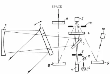
1989; Murray eta/., 1991]. Figure 2.1 is an optical diagram of the instrument. Incoming
radiation flux reflected off a scanning mirror (1), a parabolic mirror (2), and a mirror with
--The Instrument, the Data Set, and Validation 8
SPACE
Figure 2.1: Optical block diagram of the Termoskan instrument. 1 - Scanning mirror; 2
-parabolic mirror; 3 - mirror with hole in center; 4 - IR filter, reflects visible light and
transmits IR; 5 - thermal infrared detector; 6 - rotating visible channel modulator; 7
-visible channel detector; 8, 9 - spherical mirrors used in the thermal channel calibration
process; 10- black body calibrator; 11 -protective glass over the opening used for thermal
channel calibration to space; 12 - visible channel calibration lamp; 13 - mirror; and 14
[image:27.559.60.435.246.499.2]-9 2.2 The TermoskLin Instrument
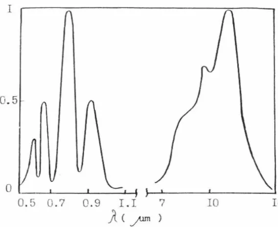
the infrared detector (5) and reflected visible radiation to the visible channel detector (7).
Figure 2.2 shows Termoskan's spectral response, which is reproduced in tabular form in
Appendix 3.
Two dimensional images were acquired one thermal-visible pixel pair at a time
through the combined action of the scan mirror and the spacecraft motion. The
displacement of the instantaneous field of view by the scanning mirror provided line
scanning in the direction perpendicular to the spacecraft motion vector. Frame scanning
resulted from the orbital motion of the spacecraft. The instrument was fixed to the
spacecraft, i.e., there was no scan platform.
The Termoskan instrument had an instantaneous field of view of 0.9 minutes of
arc, a full scan angle of 6.1°, and a scanning frequency of one line per second. Data were
only taken in one direction (roughly north to south in the observations). Most of the one
second per line involved the actual taking of Mars data. A small fraction of the time was
needed to reset the mirror. The instrument arrangement allowed a swath width of 650 km
and a best resolution of 1.8 x 1.8 km per pixel from an altitude of 6300 km. The duration
of each survey session detennined the length of each panorama. Table 2.1 summarizes the
optical and signal characteristics of the Termoskan instrument
The calibration of the infrared channel was fine tuned using an on-board black
body (10) at 310
±
0.1 K, as well as observations to open space (11) to detennine a zerolevel. Sampling of the black body and space were carried out after every eight data pixels
via a rotating modulating chopping wheel (14).
The base level for the visible channel calibrations was determined during the return
phase of the scan mirror after each line of data was taken, i.e., once per second. This was
done using a black area on the rotating visible modulator (6). The amplification factor for
the visible channel calibration could be set from the ground to a fixed value, or adjusted
according to the signal from the visible calibration lamp (12). The calibration lamp could
The Instrument, the Data Set, and Validation 10
I
0
0.5 0.7 0.9 I.I 7 10 14
) < p )
[image:29.558.106.390.219.451.2]SPECTRAL CHARACTERISTICS
-11 2.3 The Observations
however, the signal from the calibration lamp (12) was never used. Only fixed
amplification factors were used. Thus, the calibration of the visible channel was more
dependent than the thermal channel upon pre-flight calibration, plus some refinement
during the cruise to Mars. Figure 2.3 shows the calibration of the thermal channel, which
[image:30.558.57.384.201.499.2]is reproduced in tabular form in Appendix 3.
TABLE 2.1: Tennoskan Instrument and Signal Parameters
Weight 28 kg
Aperture 150mm
Focal length 375mm
Scan nue 1 line/second
Scan angle + 3.0 degrees
Instantaneous Field of View 0.26 mrad per pixel
Infrared deteaor HgCdTe
Visible deteaor Photodiode Si
Spectral Bands: Visible 0.5 -0.95 microns
Infrared 8.5 -12.0 microns
Data pixels per line 384
Calibration: Visible Onboard lamp
Calibration: Infrared Onboard black body and space
Bits per pixel 8
Ternpera!Ure sensitivity (K) 0.5 at 240 K
Temperature range (K) 170-290
There is noise equivalent to approximately 1-2 degrees Kelvin in every 8th sample of the infrared
images.
2.3
The Observations
Four Termoskan observing sessions were carried out. Each provided a thermal
emission and a visible panoramic view of the surface. Details of the panoramas are
summarized in Table 2.2. Originally, the main purpose of the sessions was to refine the
calibration of the instrument. When the spacecraft failed, however, their value obviously
The Instrument, the Data Set, and Validation 12
0 l()
z o I
8 o 0:::
w
m
:::2
:::> z
<(
~
0
0
If)
TERMOSKAN THERMA_ RESPONSE CHARACTERISTICS
BRIGHTNESS TEM0ERATURE (K)
-3 !» 0" 0 N i--.> (/.)
~
e; '-<: 0....,
~ "'1 3 0 C/) 7;'" § t) !»s
(/.) 0 ... TI\BLE 2 : SUMMARY OF TERMOSKAN DATA SETStart Time (UT) Stop Time (UT)
Total Morning Evening Phobos Local Minimum Resolution Altitude per pixel Number Limb Limb Shadow
Date M
-D-Y Ls Wes t ~ime of in in in Scan h m s h m s Longitude Latitude of Day (km) (km) Lines scan scan scan 1A 2-11-89 10 55 00 11 26 0 4 357 80-240 6N-4S 6 . 0-18 . 0 1150 . 3 1864 No No No 18 2-11-89 lO 55 00 11 26 0 4 357 80-240 6N -4 S 6 . 0 -18 . 0 1150 . 3 18 64 Yes No No 2 A 3 -0 1 -89 13 1 2 00 13 52 00 6 317-0 -49 5N-12S 9 . 6-16 . 5 6300 1 . 8 2400 N o N o N o 2B 3 -01 -89 13 12 00 13 34 50 6 4 -49 5N -8S 9 . 6-13.0 6300 . 8 13 70 N o N o No ) A 3-26 -89 09 11 29 1 0 11 29 18 5-170 7S-30S 6 . 3-17 . 6 6300 1 . 8 3600 Yes Yes Yes 3 8 3 -26-89 09 11 29 10 11 29 18 5-170 7S-30S 6 . 3 -17 . 6 6300 1.8 3600 Yes Yes Yes 4P, 3 -26 -89 1 6 48 30 17 49 50 18 115-280 7S-30S 6 . 3-17 . 6 6300 1.8 3680 No No Yes 48 3-26 -89 16 48 30 17 23 30 18 185 -280 7S-30S 6 . 3 -17 . 6 6300 1 . 8 2100 Yes No Yes Termoskan acquired a total of 4 strips across Mars . In the above chart, A designates infrared data, and B designates visible data ; e.g . , scans 1A and 18 were acquired simultaneously with 1A consisting of infrared data and 18 consisting of data from the visible channel . Start and stop times given are times at the space craft, not ground receive times . All scans were acquired in 3 axis, sun-star stabilized mode . There was no scan platform . Termoscan l oo ked along the Sun-spacecraft line (i . e . , zero phase angle), except for slight rocking motions of the spacecraft . Because Scan 1 was acquired near the periapse of one of the early elliptical orbits, the scan is very undersampled .
-w ;;l
"'
a
0" ""'"'
~
6
·
;:, ""'The Insttument, the Data Set, and Validation 14
February 11 and March 1, and two on March 26. These dates corresponded to
areocentric solar longitudes CLs) of 356°, 6°, and 18°, respectively. These occur near the
beginning of northern spring (Ls
=
0°) on Mars. The four slightly overlapping thermalpanoramas (also called scans or swaths) cover a large portion of the equatorial region
from 30°S to 6°N latitude (Figure 2.4). Simultaneous visible panoramas were taken
during each of the four observing sessions; due to spacecraft memory limitations, visible
channel processing was stopped early relative to the thermal channel for two of the
sessions (panoramas 2 and 4). Thus, the visible panoramas are shorter than the thermal
panoramas for these sessions (Table 2.2).
Termoskan's best resolution per pixel was 1.8 km for three of the panoramas
acquired and 300 m for the remaining panorama (taken on February 11). These
resolutions per pixel are much better than those obtained by the Viking infrared thermal
mapper (IRTM) (approximately 5 to 170 krn/pixel, with only a small fraction of the data
near 5 krn/pixel, and with a typical value of 30 krn/pixel [Christensen, 1986]).
Termoskan's spatial resolution is also better than the 3 krn/pixel expected for Mars
Observer's thermal emission spectrometer (TES), although TES observations will provide
global2 p.m. and 2 a.m. local time as well as spectral coverage.
During the Termoskan observations, the Phobos spacecraft was in the mode of
continuous sun - star orientation. Fixed to the spacecraft, Termoskan pointed in the
anti-solar direction during all observing sessions. Thus, all observations are at nearly 0° phase
angle and only daytime observations were acquired.
Scan lines were acquired going approximately from North to South on the planet
at a rate of 1 line per second. Each image consists of 384 samples. The number of lines
varied depending upon how long the instrument was on in any given panorama (Table
2.2). Data taking progressed from west to east due to the spacecraft motion. The data
are 8 bit data with dn (data number, i.e., signal) values able to range from 0 to 255 for
0
0
(I) H
0
r--N
0 M
0
M
0
- '
0
I
I
I
I
'
'\ 150
7
7
1
I
1
I
\
\
\
\
0
7
\0l:'-I
0
0
(])
0
(X)
H
0
r--N
[image:34.564.116.366.75.656.2]The Observations
The Instrument, the Data Set, and Validation 16
During the February 11 session (panorama 1 ), the Phobos spacecraft was in an elliptical transfer orbit with a minimum distance to the observed planet of only 1150 km. The thermal emission and reflected light profiles exhibited longitudinal gaps of varying
sizes between scan lines. Each scan in the North - South direction, however, maintained
full coverage and resolution, which was 300 m/pixel. The remaining three sessions were taken from a circular orbit closely similar to that of the moon Phobos with an altitude of
6300 km. For these panoramas, line and frame scanning correspond; therefore, there are not significant gaps between scan lines, and geometrical distortions primarily occur only
because of the sphericity of the planet. Each of the two observing sessions on the 26th of
March lasted one hour. This interval was sufficient for Termoskan to cover the Martian
surface from limb to limb. Atmospheric limb studies are discussed in Chapter 5. Also in
these two sessions, Termoskan imaged the shadow of Phobos on the surface of Mars as discussed and analyzed in Chapter 6.
2.
4 The Data Files
The Termoskan instrument was built and operated by the Institute of Space
Devices Engineering (ISDE) in Moscow. In April 1990, ISDE delivered the Termoskan data set to Caltech in the form of 23 digital files. These 23 files were incorporated,
essentially as delivered, onto the Planetary Data System (PDS) Phobos '88 CD-ROM and are referred to here as the raw data set (PDS DATA_SET_ID
=
PHB2-M-TS-2-THERMNIS-IMGEDR-Vl.O). They are described in Appendix 2 which is taken from material provided to the PDS for inclusion on the CD-ROM [Betts, 1992]. The only
significant difference between the CD-ROM raw data set and the one that was delivered by ISDE to Caltech is that I mirror flipped some ftles. This was necessary because some of the image files were delivered to Caltech with Mars appearing as it would in a mirror.
The delivered raw data set contained many other complexities that hampered
17 25 Contrast in the Visible and Thermal Channels
the thermal and visible channels in both lines and samples. I altered these original files to
produce a set of more readily usable and scientifically coherent edited files. These files
[Betts, 1992] were also included on the PDS Phobos '88 CD-ROM. To produce these
files, I combined the raw file fragments into the eight whole panoramas (four thermal and
four visible); added blank lines to correct geometrically for dropped lines; and adjusted for
misalignment of the thermal and visible channels in both lines and samples.
This edited data set was used for the analyses presented in this thesis. Appendix 1
lists all the data files and naming conventions from the CD-ROM. Appendix 2 includes
the data set descriptions I prepared for the PDS CD-ROM for both the raw and edited
files. Readers interested in actually using the data, or just after a more detailed
understanding of the creation of the edited data files, their organization, and their
complexities are urged to read Appendix 2. Particularly for the edited data set, note the
data set description. It discusses how the files were created. Also, see the confidence
level notes, which present information about noise within the data, both periodic and
random, and about accuracy of alignment
2.5 Contrast in the Visible and Thermal Channels
A conspicuous attribute of the Termoskan panoramas is the much lower contrast
in the photographic displays of the visible channel versus the thermal infrared. Indeed, this
difference is even more striking when viewed in the unstretched digital data, for example,
in Figure 5.2. A major factor contributing to the low visible contrast in the visible is the
zero phase angle nature of the observations. Shadows on the Martian surface arising from
large-scale relief and from topographic slopes were not visible.
In addition, Viking data analyses emphasized how atmospheric dust and other
aerosols will cause a lack of surface contrast at visible wavelengths [e.g., Thorpe et al.,
1979]. Thus, scattering by dust and ice crystals in the Martian atmosphere also may
The Instrument, the Data Set, and Validation 18
contrast between the visible and infrared channels implies that the visible wavelength
optical depth is probably significantly larger than the thermal infrared optical depth. This
is consistent with the results of Toon et al. [1977], Pollack et al. [1979], Martinet al.
[1979], and Zurek et a!. [1982] Their Mariner 9 and Viking analyses imply visible to
infrared optical depth ratios for this season of order 2 or greater.
Analyses of limb profiles and of Phobos shadow images, discussed in Chapters 5
and 6, respectively, show that instrumental scattering in the Termoskan optics was
negligible. Rocket propulsion products and induced vibrations always pose the threat of
fine dust contamination of space optics. Thus an in-flight demonstration of the absence of
instrumental scattering is very desirable.
Fortunately for scientific studies of Mars surface, the thermal emission channel
yielded very high contrast data. This attribute is clear not just in the photographic
renditions, but in the actual digital data as, for example, in Figures 2.7, 2.8, and 2.9. This
circumstance reflects in part the excellent qualities of the instrument itself. The
Modulation Transfer Function of the entire Termoskan system must have been very high
in order for abrupt pixel-to-pixel variations in signal to be recognized. In addition, the
bulk of Mars' atmospheric scattering at visible wavelengths probably arises from particles
in the half micron or less range [Clancy and Lee, 1991]. These are too small and too cold
to be discernible emitters in the 8 to 13 micron region (except at the limbs, where path
lengths are greater). Furthermore, the dominantly high-sun observational conditions of the
Termoskan images enhance the visibility of thermal differences arising from albedo,
texture, and slope variations. Modelling studies predict variations of tens of Kelvins.
2.6
Data Validation: Comparison with IRTM
Determining the absolute accuracy of the Termoskan thermal data was a critical
first step towards understanding the usefulness and believability of the data set. Validation
19 2.6 Data Validation: Comparison with IRTM
prematurely short. Understanding the accuracy of the thermal channel proved important for many of the later studies presented here, particularly those that attempt to calculate
thermal inertias (e.g., for channels in Chapter 4 and using the Phobos shadow in Chapter 6).
The kinetic temperature of a surface cannot be directly measured by a remote
sensing instrument such as Termoskan. Instead, brightness temperatures are derived from
the thermal infrared signal assuming black body surface emission. All further references to
temperature within this thesis refer to brightness temperature.
In order to independently test the accuracy of the thermal channel, I compared
Termoskan brightness temperatures to brightness temperatures from Viking's infrared
thermal mapper's (IRTM's) 11 micron channel (9.8 to 12.5 pm). I constrained the IRTM data to match approximately the Termoskan data in season <Ls), longitude, latitude, and local time of day. In selecting the constraints, I had to balance matching those parameters
accurately with obtaining a statistically significant number of IRTM points. Some of the largest overlap with IRTM data occurred in panorama 3, upon which I focus here. Figure
2.5 shows the latitudes and longitudes of IRTM points that match points within a section of panorama 3 to within ±1 0° of Ls and ±30 minutes of surface local time. Presented here are comparisons for two strips within panorama 3. The locations of the centers of the strips are shown superimposed on Termoskan data in Figure 2.6.
Figure 2.7 shows a comparison of IRTM and Termoskan data for a strip of
constant latitude that is two degrees wide and centered upon l8°S latitude. In order to
compare the two data sets, I degraded the Termoskan resolution to a resolution comparable to Viking. Thus, in Figure 2.7 the dark line represents Termoskan data that
have been averaged in 67 x 67 pixel squares (approximately 2° x 2°). The thinner line is a
one pixel Termoskan strip for reference. The IRTM data are represented by dots with
The Instrument, the Data Set, and Validation 20
0
0
~ ..._) I
0
::>
>-5
01
~f
r
0
r')
1180
LOCATIONS OF IRTM DATA CORRESPONDING TO SCAN 3, WITHIN 30 MIN. LOCAL TIME
160 140 120
WEST LONGITUDE
: ... ·
.
.
·..
. . .
. · .· . . · . . .
100
Figure 2.5: Plotted are the locations of the IRTM points which match this section of
[image:39.567.42.451.216.531.2]21 2.6 Data Validation: Comparison with IRTM
Figure 2.6: Termoskan visible (top) and thermal (bottom) images centered approximately upon l4°S, ll7°W. North is top. In all the thermal images in this thesis, darker is cooler.
The two lines in the IR data represent the center lines of the strips of data which are compared with IRTM data in Figures 2.7 (southern line) and 2.8. The Phobos shadow
used for the analyses in Chapter 6 can be seen within the boxed portion of the visible data
The Instrument, the Data Set, and Validation 22
0 lD
N
I
0.: :2 c ..,- I[
w "'
L
< _J n Ntl
m0
N
-"- L
135
d: - 18?0± i ?0 LAT.; ERMO. DATA: 6 7 P•XELS SQUARE AVG .. ± 30 M '\
AVERAGE TEMPERATURE DIFFERENCE
BETWEEN TERMOSKAN AND IRTM:
3.1 ± 0.4
130 125 120 1 iS 110
WEST LOI'<GITUDE
105
Figure 2.7: Comparison of Termoskan data with analogous IRTM data for a 2 degree
wide strip of constant latitude centered on 18°S. The dark line represents a sliding boxcar
average of Termoskan data which has been averaged in 2° x 2° squares. The thinner line
is a 1 pixel Termoskan strip for reference. The points represent IRTM data with the error
bars representing the footprint of each IRTM data point. IRTM data is constrained to
match the Termoskan data to within ±10° of Ls and to within ±30 minutes of local time.
Local time of day in the data shown ranges from about 8.5 to 10.3 H. After comparing
each IRTM point with the averaged Termoskan point of the same longitude, the average
temperature difference between Termoskan and IRTM is 3.1±0.4 K with the Termoskan
temperatures being warmer. Note how the large scale qualitative features match in the
Termoskan and IRTM data. The lower line in the infrared image shown in Fig. 2.6
c ID-"' t
~
z 0 0 _., -C.:: N
u ~
>-0 0 m
:.:: u o < ""
-as
"'
~
r
.
o '1.35
23 2.6 Data Validation: Comparison with IRTM
d -9~5± 1 °C LA-.. Tf:R\10. DA-t, S 67 PIXeLS SGUARE AVG.; =.30 Mli''l
AVERAGE TEMPERATURE
D
I
FFERE
NC
E
~
BETWEEN TERMOSKAN A D IRTM:
L
3.2 ± 0.5
130 125 120
WEST LOI\GITUDE
• 15 110 105
Figure 2.8: Analogous plot to Figure 2.7 for 9.5°S
.
The upper line in the infrared
image
The Instrwnent, the Data Set, and Validation 24
data point. Local times of day in these data range from about 8.5 to 10.3 H (24 H
=
1 Martian day).After comparing each IRTM point with the averaged Termoskan point of the same longitude, the average temperature difference between Termoskan and IRTM is 3.1
±
0.4K with the Termoskan temperatures being warmer. Also significant, note in Figure 2. 7
that qualitative features match well between the two data sets. Figure 2.8 shows an
analogous graph centered upon 9.5°S. For these data the average temperature difference
is 3.2
± 0.5
K. This result is consistent with the results obtained from the data in Figure 2.7 and from other latitudinal strips that I have examined.The approximate 3K difference also includes the effects of the somewhat different
bandpasses of the Termoskan IR channel and the Viking IRTM 11 Jlm channel [Kieffer et
al., 1977]. The peak of the Termoskan response actually falls between the peaks of the
IRTM 9 Jlm and 11 Jlm channels. I compared Termoskan with sparsely available IRTM 9 Jlm data as well. For the regions studied, the IRTM 9 Jlm brightness temperatures average about 1.5 K higher than the IRTM 11 Jlm brightness temperatures. Thus, the average temperature difference between Termoskan and the IRTM 9 Jlm channel is closer
to 1 or 2 K. I conclude that the Termoskan brightness temperatures probably differ by no
more than 2 K from comparable IRTM data.
One significant cause of the differences between IRTM and Termoskan is the
difference in phase angle. IRTM measurements were in general taken at much higher
phase angles than the near 0° phase angle Termoskan measurements. In particular, all of the IRTM data shown in Figures 2.7 and 2.8 was taken between 34° and 36° phase.
Looking at 0° phase angle, Termoskan observed only the sunlit sides of surfaces and did not observe currently shadowed areas. The IRTM observations, taken at similar times of day, but at much higher phase angles, would have observed shadowed areas. In addition,
IRTM would have observed the cooler sides of objects. This is a significant effect
25 2.7 Albedo and Thermal Inertia Determinations depth is much smaller than the object [Jakosky et al., 1990]. The magnitude of the phase angle induced differences could be a few degrees Kelvin [Jakosky et al., 1990].
Even ignoring possible errors in the decalibrated Viking IRTM data, there are
other possible sources of the offset between Termoskan and IRTM. These include any bias in the Termoskan absolute preflight calibration, and any intrinsic difference in Mars' thermal emission between 197 6-7 8 and 198 9, including atmospheric effects such as clouds.
Not only are absolute temperature differences very small between Termoskan and
IRTM, but also the thermal features in the Termoskan data qualitatively correlate very
well with the lower resolution IRTM data, as seen in Figures 2.7 and 2.8. Thus, in both
an absolute and a relative sense, I have a high degree of confidence in Termoskan's thermal channel and its calibration.
Termoskan sees thermal variations even at the limit of its spatial resolution. Figure 2.9 again shows Termoskan and IRTM data for 18°S latitude. The three curves represent different degrees of spatial averaging of the Termoskan data. Curve 1 is not averaged,
i.e., it is a 1 pixel wide strip; curve 2 has 11 pixels averaged in a north-south direction; and curve 3 has 67 pixels averaged in a north-south direction. None of the curves are
averaged in an east-west direction (whereas, Figures 2.7 and 2.8 were). Thermal features
remain at the limit of resolution of the 1 pixel curve. For example notice the spike at approximately 115°W longitude (in Figure 2.9). This corresponds to the sunlit rim of a 6 km diameter crater.
2.7 Albedo
and Thermal Inertia Determinations
Almost all of the analyses presented in this thesis involve the derivation of thermal properties of the surface, because the power of Termoskan lies in its high spatial
resolution in the thermal infrared. Its visible spatial resolution is far worse than that of the
The Instrument, the Data Set, and Validation 26
0 ...
N
0
<D
N
z 0 0 l{l IX N
u
-~if
a.. 0 :2 """ ~ ('.;>-0
0 CD
d: -18?0± 1 ?0 LA.T.; PIXELS WIDE= 1. 11,67; ±30 MIN. TOO
. - ----'--- l
'30 120 110
WEST LOf\:GITUDf
Figure 2.9: The lines represent Termoskan data centered upon -18 degrees latitude. Curve 1 (top) has no averaging; it is a 1 pixel wide strip to which 10 K have been added uniformly to ease comparison with the other curves. Curve 2 (middle) has 11 pixels averaged in a north-south direction. Curve 3 (bottom) has 67 pixels averaged in a north-south direction and has had 10 K subtracted from it. Note that sharp features can be seen
in the 1 pixel wide strip that average out at lower resolutions, e.g., the spike at
27 2.7 Albedo and Thermal Inertia Determinations
interested in whether the visible channel signal can be converted to bolometric Bond
albedo, which is the parameter necessary for the derivation of thermal properties.
Thermal inertia and bolometric Bond albedo are the two most important physical
properties of a planetary surface that determine its diurnal temperature variations.
Thermal inertia, a bulk measure of the resistance of a unit surface area to changes in
temperature, is commonly used to characterize the insulating properties of planetary
surfaces. It is defmed as I= (kpcp)l(l. where k is the thermal conductivity, pis the density,
and Cp is the specific heat. Low inertia materials exhibit the largest day-to-night surface
temperature variations and the smallest thermal skin depths.
For the martian surface, thermal inertia is often expressed in units of 1Q-3 cal cm-2
K-1 sec-112 (e.g., in Kieffer et al., 1977). As a matter of convention, these units are used
for thermal inertias throughout this thesis. To convert to SI units (J m-2 K-1 sec-112),
multiply by 41.86. Several authors (e.g., Kieffer et al., [1977]; Palluconi and Kieffer,
[1981]; and Haberle and Jakosky [1991]) have used brightness temperatures and thermal
modelling to derive thermal inertias for the martian surface. These authors used IRTM
data from multiple times of day to derive both inertia and bolometric albedo
simultaneously.
T~rmoskan observed only a small area at more than one local time of day and
those data are badly foreshortened. Thus, for essentially all the Terrnoskan data, inertias
and albedos cannot be derived independently using observations at two times of day.
Therefore, the majority of the Termoskan data require bolometric albedo for thermal
inertia determinations. Accurate bolometric albedos are particularly important for deriving
inertias from Terrnoskan data because only daytime observations were obtained. Daytime
temperatures are very dependent upon bolometric albedos.
Bolometric (Bond) albedo defmes the fraction of incoming solar flux over all
wavelengths that is not absorbed by a surface. Surfaces with high bolometric albedos
The Instrument, the Data Set, and Validation 28
("dark" swfaces). Bolometric Bond albedo for a unit surface element is most simply defined as:
A=
pf
q(a)dawhere p is the total reflectivity of all wavelengths at 0° solar phase angle, a., and q(a.) is
the variation of reflectivity over all wavelengths with increasing solar phase angle for the
swface element Even the most comprehensive Mars albedo observations are limited by uncertainties in the local variation in q, in wavelength dependence, and in temporal and
spatial variations in atmospheric scattering. Termoskan observed only the total visible
intensity from Mars swface elements at a.
=
0°. The visible intensity observed includedboth swface and atmospheric components. Because Termoskan essentially did not
observe shadows due to its zero phase angle geometry, the atmospheric contribution
cannot be removed using the observed flux in shadowed areas as has been done with other data sets [e.g., Herkenhoff, 1989]. In addition to the other difficulties, the visible Termoskan data are largely dependent upon pre-flight calibration. Thus, even approximate estimates of Bond albedo from the Termoskan visible data alone will yield
only low confidence results.
Another possible way to gain confidence in bolometric albedos derived from
Termoskan data would be tying them to bolometric albedos derived from Viking IRTM
solar band measurements. To test this possibility, I compared 1 o x 1 o averaged Termoskan dn (signal) values with the corresponding 1 o x 1 o binned albedos of Pleskot
and Miner [1981]. Comparison strips were limited in latitude and longitude to lessen geometric and atmospheric effects. This increased the chances of tying the Termoskan data to the Viking albedos.
29 2.7 Albedo and Thermal Inertia Determinations
1 X 1 DEGREE TERMOSKAN ON AVERAG:::S VS. IRTM DERIVED 1 X 1 ALBEDOS
~ .---~--~--~--~--~--~--~---~--~--~--~--~---~
0
L{)
c)
~
0 ~--L---L---L---~--~--~--~--~---L--~---L--~--~--~--_J
60. 80 100 120 140 160 180 200
TERMOSKAN ON VALUE
Figure 2.10: Termoskan visible dn vs. IRTM albedos - high contrast. Dots represent Termoskan 1° x 1° averages of visible channel dn (signal) values plotted versus IRTM I 0
x 1° bolometric albedos from Pleskot and Miner [1981]. The bin centers range from 3.5°N,
42.5°W to 4.5°S, 31.5°W. Note the large amount of scatter in the plot. The line