Victor E. Ambrus,∗
Department of Physics, West University of Timis,oara,
Bd. Vasile Pˆarvan 4, Timis,oara, 300223, Romania Elizabeth Winstanley†
Consortium for Fundamental Physics, School of Mathematics and Statistics,
The University of Sheffield, Hicks Building, Hounsfield Road, Sheffield, S3 7RH, United Kingdom
(Dated: December 17, 2015)
We study a quantum fermion field inside a cylinder in Minkowski space-time. On the surface of the cylinder, the fermion field satisfies either spectral or MIT bag boundary conditions. We define rigidly rotating quantum states in both cases, assuming that the radius of the cylinder is sufficiently small that the speed-of-light surface is excluded from the space-time. With this assumption, we calculate rigidly-rotating thermal expectation values of the fermion condensate, neutrino charge current and stress-energy tensor relative to the bounded vacuum state. These rigidly-rotating ther-mal expectation values are finite everywhere inside and on the surface of the cylinder and their detailed properties depend on the choice of boundary conditions. We also compute the Casimir divergence of the expectation values of these quantities in the bounded vacuum state relative to the unbounded Minkowski vacuum. We find that the rate of divergence of the Casimir expectation values depends on the conditions imposed on the boundary.
PACS numbers: 03.70.+k, 04.62.+v
I. INTRODUCTION
The definition of quantum states is of central impor-tance in quantum field theory (QFT) on both flat and curved space-times. Of the possible quantum states on a given space-time, defining a (not necessarily unique) vacuum state is essential, as states containing particles can be built up from a vacuum state using particle cre-ation operators. Even in flat space-time, the definition of a vacuum state is nontrivial when the space-time con-tains boundaries or one is interested in the definition of particles as seen by a noninertial observer.
To define a vacuum state in the canonical quantiza-tion approach to QFT, one starts with an expansion of the quantum field in terms of a basis of orthonor-mal field modes. These modes are split into “positive” and “negative” frequency modes. For a quantum scalar field, this split is not completely arbitrary; it must be the case that positive frequency modes have positive Klein-Gordon norm and negative frequency modes have neg-ative Klein-Gordon norm. For a quantum fermion field, all modes have positive Dirac norm and the split between “positive” and “negative” frequency modes is much less constrained.
This difference between quantum scalar and fermion fields was explored in [1] for rigidly-rotating fields on un-bounded Minkowski space-time. For a quantum scalar field, the norm of a field mode is proportional to the Minkowski energy E of that mode. As a consequence, positive frequency modes must have positive Minkowski
∗[email protected] †[email protected]
energy and the only possible vacuum state is the (non-rotating) Minkowski vacuum [2]. For a quantum fermion field, two possible vacua have been considered in the lit-erature: the nonrotating (Vilenkin) vacuum [3] and the rotating (Iyer) vacuum [4]. To construct the nonrotating vacuum, positive frequency fermion modes have positive Minkowski energyE as in the scalar field case. For the rotating vacuum, positive frequency fermion modes have positive corotating energyEe (the energy of the mode as
seen by an observer rigidly-rotating about thez-axis in Minkowski space-time with angular speed Ω). In gen-eralE 6=Ee for a particular field mode. On unbounded
Minkowski space-time, there exist fermion field modes with EE <e 0, which means that the nonrotating and
rotating vacua are not equivalent [1].
Rigidly-rotating thermal states on unbounded Minkowski space-time can be defined from the above vacuum states. The rigidly-rotating nature of these states means that the thermal factor in the thermal Green’s functions and corresponding expectation values involves the corotating energy E.e For a quantum
scalar field, rigidly-rotating thermal states are divergent everywhere in the unbounded space-time [3, 5]. The density of states factor in the thermal expectation values (t.e.v.s) for a bosonic field isheβEe−1
i−1
, whereβ is the inverse temperature. This thermal factor diverges when the corotating energy Ee vanishes, even though such
modes are nonzero in general [5]. Modes with vanishing corotating energy therefore make an infinite contribution to rigidly-rotating t.e.v.s, leading to divergences.
One way to resolve this difficulty is to enclose the sys-tem in an infinitely long cylinder of radius R, with the axis of the cylinder along thez-axis and ΩR < c, where
c is the speed of light. For this range of values of R, the boundary of the cylinder is inside the speed-of-light surface (SOL) (the surface on which an observer rigidly-rotating about the z-axis with angular speed Ω must travel at the speed of light). With the SOL removed from the space-time, it can be shown thatEE >e 0 for all
scalar field modes, so that the modes which lead to di-vergences in t.e.v.s on unbounded Minkowski space-time are absent [6]. The resulting rotating t.e.v.s for a quan-tum scalar field on the space-time inside the cylinder are regular everywhere inside and on the boundary of the cylinder [5].
Rigidly-rotating thermal states for a quantum fermion field on unbounded Minkowski space-time were studied in [1] and exhibit different behaviour from those for a quantum scalar field. Rigidly-rotating t.e.v.s are regular inside the SOL and diverge as the SOL is approached. If the nonrotating (Vilenkin) vacuum is used, then t.e.v.s contain spurious temperature-independent terms [1, 7] which are unphysical since t.e.v.s with respect to the vacuum state should vanish in the limit of zero tempera-ture. These temperature-independent terms vanish if the rotating (Iyer) vacuum is used instead [1].
In this paper, we study the fermionic analogues of the rotating thermal states inside a cylinder, studied for the scalar case in Ref. [5]. We construct rigidly-rotating quantum states for Dirac fermions enclosed inside an in-finitely long cylinder in Minkowski space-time. The axis of the cylinder is along the axis of rotation, thez-axis. On the boundary of the cylinder, the fermions satisfy either spectral boundary conditions [8] or one of two versions of the MIT bag boundary conditions, the standard [9] and chiral [10] MIT bag models. In each case, we find that the rotating and nonrotating vacua coincide when the boundary of the cylinder lies within the SOL. We com-pute rigidly-rotating t.e.v.s of the fermion condensate, neutrino charge current and stress-energy tensor for each set of boundary conditions, comparing the results with those in [1] for the unbounded space-time. We also study Casimir expectation values, namely the expectation val-ues for the bounded vacuum state relative to the (non-rotating) vacuum state on unbounded Minkowski space-time. Our Casimir expectation values for a fermion field are compared with those in [5] and [11] for a quantum scalar field and for fermions obeying MIT bag boundary conditions, respectively.
The outline of this paper is as follows. In Sec. II, we review the construction of mode solutions of the Dirac equation in unbounded Minkowski space-time, the sec-ond quantization procedure and the definition of the ro-tating and nonroro-tating vacuum states. For the remainder of the paper we consider the bounded space-time. For the spectral and MIT bag boundary conditions, in Sec. III, we study mode solutions of the Dirac equation satisfy-ing the boundary conditions, their energy spectra and the construction of the vacuum state. Rigidly rotating thermal expectation values are computed in Sec. IV and the Casimir effect is analysed in Sec. V. Finally, Sec. VI
contains some further discussion.
II. UNBOUNDED SPACE-TIME
In this section, we review the construction of mode solutions and vacuum states in a rigidly rotating, un-bounded, Minkowski space-time [1]. The Dirac equation is introduced in Sec. II A, while the construction of its so-lutions is presented in Sec. II B. The section closes with a discussion of the choice of vacuum state on the un-bounded space-time in Sec. II C.
A. Dirac equation in rotating Minkowski space-time
The world line of an observer rotating with a constant angular velocity Ω about thez-axis can be parametrized in cylindrical coordinates as xµ = (t, ρ,Ωt, z) for fixed ρ and z. The coordinate frame with respect to which the observer is at rest can be obtained from the usual Minkowski coordinatesxµMby settingϕ=ϕM−Ωt. The Minkowski metric then takes the form:
ds2=−(1−ρ2Ω2)dt2+ 2ρ2Ωdt dϕ+dρ2+ρ2dϕ2+dz2. (2.1) Throughout this paper we use units in which c = ~ = kB = 1. The Killing vector ∂t, defining the corotating HamiltonianH =i∂t, becomes null on the speed-of-light surface (SOL), which is defined as the surface whereρ= Ω−1.
To construct the Dirac equation, we introduce the fol-lowing tetrad in the Cartesian gauge [12]:
eˆt=∂t−Ω∂ϕ, eˆi=∂i,
ωˆt=dt, ωˆi=dxi+ (Ω×x)idt, (2.2) with respect to which the Dirac equation for fermions of massµreads:
iγαˆDαˆ−µψ(x) = 0. (2.3) The gamma matrices are in the Dirac representation [13]:
γˆt=
1 0 0 −1
, γˆi=
0 σi
−σi 0
, (2.4)
where the Pauli matricesσi are given by:
σ1=
0 1 1 0
, σ2=
0 −i i 0
, σ3=
1 0 0 −1
. (2.5)
The gamma matrices obey the following canonical anti-commutation rules:
n
whereηαˆβˆis the inverse of the Minkowski metric η ˆ αβˆ= diag(−1,1,1,1). We use the convention that hatted in-dices denote tensor components with respect to the or-thonormal tetrad introduced in Eq. (2.2) and are raised and lowered using the Minkowski metricηαˆβˆ.
The covariant derivativesDαˆin Eq. (2.3) are given by: iDˆt=H+ ΩMz, −iDˆj=Pj. (2.7) In the above, H = i∂t is the corotating Hamiltonian, Pj=−i∂j are the momentum operators and
Mz=−i∂ϕ+ 1 2
σ3 0 0 σ3
(2.8)
is thez-component of the angular momentum operator.
B. Mode solutions
The rotating system under consideration is just Minkowski space-time written in terms of corotating co-ordinates. Therefore mode solutions of Eq. (2.3) can be obtained from any complete set of mode solutions found on Minkowski space by applying a suitable coordinate transformation. Mode solutions of the Dirac equation on Minkowski space with respect to cylindrical coordinates have been reported in Refs. [1, 3, 4, 11, 14–18].
In this paper, we follow Ref. [1] and construct the solutions of the Dirac equation (2.3) as simultaneous eigenvectors of the complete set of commuting opera-tors{H, Pz,Mz, W0}, where the helicity operatorW0= P ·M/p is the time component of the Pauli-Lubanski vector, withP the momentum operator andMthe an-gular momentum operator. The helicity operatorW0has the following form:
W0=
h 0 0 h
, h= σ·P
2p , (2.9)
wherepis the magnitude of the momentum.
To solve the eigenvalue equations corresponding to the above operators, the eigenspinors Uj can be put in the form:
Uj(t, ρ, ϕ, z) = 1 2πe
−iEejt+ikjzu
j(ρ, ϕ), (2.10) where
j= (Eej, kj, mj, λj) (2.11) collects the eigenvalues of the set of operators (H, Pz,Mz, W0). In this paper, sometimes we will explic-itly keep the indexj(2.11) on various quantities; however at other times we shall suppress the indexj to keep ex-pressions manageable. Further, in some exex-pressions it will be necessary to explicitly show individual eigenval-ues in j (2.11). When this is the case, we will use the notationUλ
Ekmfor spinors.
In (2.10) the corotating energy Eej is linked to the Minkowski energyEj through
e
Ej=Ej−Ω(mj+12), (2.12) where Ej =±
q
p2
j+µ2 can be written in terms of the modulus pj of the momentum of the mode. The four-spinors uj introduced in Eq. (2.10) are eigenvectors of W0 andMz, corresponding to the eigenvaluesλj =±12 andmj+12, respectively, wheremj= 0,±1,±2, . . ..
Due to the diagonal form of W0 and Mz, the four-spinorsuj can be written as:
uj(ρ, ϕ) =
Cjupφj(ρ, ϕ)
Cdown
j φj(ρ, ϕ)
, (2.13)
whereCjupandCdown
j are constants. The angular momen-tum equation,
−i∂ϕ+12 0 0 −i∂ϕ−12
φj(ρ, ϕ) = (mj+12)φj(ρ, ϕ), (2.14) can be solved by setting:
φj(ρ, ϕ) =ei(mj+ 1 2)ϕ e
−i
2ϕφ− j(ρ) ei2ϕφ+
j(ρ)
!
, (2.15)
whereφ±j are scalar functions of ρ. The two-spinorsφj also obey the helicity eigenvalue equation:
1 2pj
kj P−
P+ −kj
φj(ρ, ϕ) =λjφj(ρ, ϕ), (2.16)
whereP±=Px±iPy are differential operators given by: P±=−ie±iϕ(∂ρ±iρ−1∂ϕ). (2.17) The helicity eigenvalue equation (2.16) can be used to show that the scalar functions φ±j satisfy Bessel-type equations:
[z2j∂z2j +zj∂zj +z
2
j−(mj+ 1)2]φ+j =0, (2.18a) [z2j∂z2
j +zj∂zj+z
2 j−m
2 j]φ
−
j =0, (2.18b) wherezj=qjρis written in terms of the transverse mo-mentum
qj =
q
p2
j−k2j. (2.19)
The solutions of Eqs. (2.18) which are regular at the ori-gin have the form:
φ+j(ρ) =N+
j Jm+1(qρ),
The operatorsP±(2.17) act like shift operators for the
angular momentum quantum numberm, i.e.:
P±eimϕJm(qρ) =±iqei(m±1)ϕJm±1(qρ). (2.21) Hence, the helicity equation (2.16) implies that
N+ j =
iqj kj+ 2λjpj
Nj−, (2.22)
enablingφj (2.15) to be written as:
φj(ρ, ϕ) = 1
√
2
pλeimϕJm(qρ) 2iλp−λei(m+1)ϕJm+1(qρ)
, (2.23)
where
p± ≡p±1/2=
s
1±k
p. (2.24)
For brevity, the indexjwas dropped from the right-hand side of Eq. (2.23). The overall 1/√2 factor in Eq. (2.23) comes from the generalized orthogonality relation [14]:
∞ X
m=−∞
φλEkm† (ρ, ϕ)φλEkm0 (ρ, ϕ) =δλλ0, (2.25)
where † denotes the Hermitian conjugate of the two-spinor.
Returning to the four-spinors (2.13), the Dirac equa-tion (2.3) can be used to constrain the constantsCjup and
Cdown j :
E−µ −2pλ 2pλ −E−µ
Cjup Cdown
j
= 0. (2.26)
Imposing the generalized completeness relation [14]
∞ X
m=−∞
uλEkm† (x)uλEkm0 (x) =δλλ0, (2.27)
gives the following expression for the spinorujintroduced into the modeUj in Eq. (2.10):
uj(ρ, ϕ) = 1
√
2
E
+φj 2λE
|E|E−φj
, (2.28)
where
E±= r
1± µ
E. (2.29)
The normalization ofuj means that the modeUj (2.10) has unit norm with respect to the Dirac inner product, which for the metric (2.1) takes the form [1]:
hψ, χi=
Z ∞
−∞
dz
Z 2π
0 dϕ
Z R
0
dρ ρ ψ†(x)χ(x). (2.30)
Anti-particle modesVj are obtained from the particle modes (2.10) through charge conjugation, i.e.:
Vj(x) =iγ ˆ 2U∗
j(x) (2.31)
and have the following expression:
Vj(t, ρ, ϕ, z) = 1 2πe
iEejt−ikjzv
j(ρ, ϕ), (2.32a) wherevj(ρ, ϕ)≡vEkmλ (ρ, ϕ) is given by:
vEkmλ (ρ, ϕ) =(−1) m
√
2 iE
|E|
E−φλE,−k,−m−1
−2λE
|E|E+φλE,−k,−m−1
!
.
(2.32b) TheVj modes can be written in terms of theUj modes, as follows:
Vj = (−1)mj iEj
|Ej|
U, (2.33)
where
= (−Ej,−kj,−mj−1, λj). (2.34)
C. Second quantization
As discussed in Refs. [1, 4], the vacuum state for the Dirac field on a rigidly rotating space-time is not uniquely defined. This nonuniqueness arises from the freedom to choose how fermion field modes are split into “particle” and “anti-particle” modes. This freedom is constrained for a quantum scalar field by the requirement that parti-cle modes must have positive Klein-Gordon norm (and anti-particle modes must have negative Klein-Gordon norm) in order for the particle creation and annihila-tion operators to obey canonical commutaannihila-tion relaannihila-tions. For a quantum fermion field, all field modes have posi-tive norm and so this split is unconstrained, leading to freedom in how particle creation and annihilation oper-ators are defined, and, correspondingly, freedom in the definition of the vacuum state [1].
Two possible choices for the vacuum state on un-bounded rotating Minkowski space-time are the (nonro-tating) Minkowski vacuum, considered by Vilenkin [3], and the rotating vacuum, introduced by Iyer [4]. For the nonrotating Minkowski vacuum, particle modes have pos-itive Minkowski energyE >0; for the rotating vacuum particle modes have positive corotating energy E >e 0,
with these two energies linked by (2.12).
Rigidly-rotating thermal expectation values (t.e.v.s) constructed with respect to the nonrotating Minkowski vacuum state contain spurious temperature-independent terms, due to the inclusion of modes satisfying E <e 0
in the set of particle modes [1]. The temperature-independent terms disappear when the rotating vacuum is considered, where modes withE >e 0 (including modes
Rigidly-rotating t.e.v.s of the fermion condensate, neu-trino charge current and stress-energy tensor are com-puted for both the Iyer and Vilenkin quantizations in Ref. [1]. It is found that, using the Iyer quantization, these t.e.v.s are regular everywhere inside the SOL, but diverge as the SOL is approached.
The difference between the Iyer and Vilenkin quanti-zation methods rests in the interpretation of the modes for whichEE <e 0, namely whether such modes are
con-sidered to be particle or anti-particle modes. For a quan-tum scalar field, enclosing the system inside a bound-ary of radius not greater than that of the SOL elimi-nates energies satisfyingEE <e 0 from the particle
spec-trum [6]. Vilenkin [3] argues that the same holds for fermions. In Sec. III, we show that this is indeed the case for spectral and MIT bag boundary conditions (defined in Secs. III B and III C respectively), for a cylindrical boundary placed inside or on the SOL. In this case the nonrotating (Vilenkin [3]) and rotating (Iyer [4]) vacua are therefore equivalent.
Assuming that there are no modes with EE <e 0 in
the particle spectrum, second quantization can be per-formed as in unbounded nonrotating Minkowski space, by expanding the field operatorψ(x) as:
ψ(x) =X j
θ(Ej)
h
Uj(x)bj+Vj(x)d†j
i
, (2.35)
where the step functionθ(Ej) ensures that the Minkowski energyEj is positive and
X
j
≡ X
λj=±12
∞ X
mj=−∞
Z
|Ej|>µ
dEj
Z pj
−pj
dkj, (2.36)
wherepjis the modulus of the momentum of a particle of Minkowski energyEj. The negative Ej values, excluded by the step functionθ(Ej) in Eq. (2.35), are included in the domain of integration in Eq. (2.36) for later conve-nience. The one-particle operatorsbjandd†jin Eq. (2.35) obey canonical anti-commutation relations:
n
bj,b†j0 o
=δ(j, j0), ndj,d†j0 o
=δ(j, j0), (2.37)
where
δ(j, j0) = δ(Ej−Ej0)
|Ej|
δ(kj−kj0)δm
j,mj0δλj,λj0. (2.38)
The vacuum state |0i is defined as that state which is annihilated by the annihilation operatorsbj anddj:
bj|0i= 0 =dj|0i. (2.39) In the next section, we shall investigate the properties of rigidly-rotating t.e.v.s for thermal states constructed from this vacuum state, for a fermion field satisfying ei-ther spectral or MIT bag boundary conditions.
III. BOUNDARY CONDITIONS
Our focus in this paper is a quantum fermion field on rotating Minkowski space-time, inside a cylinder centered on thez-axis (the axis of rotation) and having radius R. We exclude the space-time exterior to the cylinder from our considerations. ForRΩ<1 (where Ω is the angular speed about thez-axis), the cylinder lies completely in-side the speed-of-light surface (SOL), which is therefore removed from our space-time. For RΩ = 1, the bound-ary of the cylinder is the SOL. ForRΩ>1, the SOL lies within the cylinder - we do not consider this possibility. We consider two models for the implementation of boundary conditions for a quantum fermion field on the surface of the cylinder: the spectral [8] and MIT bag [9] models. In Sec. III A, the self-adjointness of the Hamil-tonian is used to derive a constraint on the behaviour of the fermion field on the boundary. Secs. III B and III C introduce the spectral and MIT bag models, respectively. For each model, the energy spectrum and corresponding vacuum states are discussed, confirming that if the SOL is not inside the boundary, the rotating and Minkowski vacua coincide.
A. Self-adjointness of the Hamiltonian
The Hamiltonian is, by definition, a self-adjoint oper-ator with respect to the Dirac inner product:
hψ, Hχi=hHψ, χi, (3.1) for any combination of solutions (ψ, χ) of the Dirac equa-tion (2.3). On a general background, the Dirac inner product is given by:
hψ, χi=
Z
V
d3x√−g ψγt(x)χ, (3.2)
whereψ=ψ†γtˆandγµ=eµαˆγαˆare the covariant versions of the gamma matrices introduced in Eq. (2.4), satisfying
{γµ, γν}=−2gµν. (3.3) ForH =i∂t, Eq. (3.1) is equivalent to:
∂thψ, χi= 0. (3.4)
This time derivative can be obtained from the Dirac equation (2.3), which reads for a general space-time as follows:
iγλ∂λψ+iγλΓλψ=µψ, (3.5) where Γλ is the spin connection [19], defined to preserve the general covariance of the gamma matrices:
[Dµ, γν] =∂µγν+ Γνλµγ λ+ [Γ
Taking into account the following properties: γt∂tχ=−γi∂iχ−γλΓλχ−iµχ, ∂tψγt=−∂iψγi+ψΓλγλ+iµψ, ∂t(
√
−gγt) =−∂i(γi
√
−g)−√−g
Γλ, γλ, (3.7) an integration by parts in Eq. (3.4) shows that
∂thψ, χi=−
Z
∂V dΣi
√
−g ψγiχ, (3.8)
where∂V is the 2-boundary of the integration 3-surface V. In our case, the integration domain is the volume contained inside an infinite cylinder of radius R and its boundary is the enclosing cylinder. Thus, the Hamilto-nian is self-adjoint only if:
R
Z ∞
−∞
dz
Z 2π
0
dϕ ψγρˆχ
ρ=R= 0. (3.9) Eq. (3.9) provides necessary and sufficient conditions for a set of boundary conditions to yield a consistent quanti-zation. In the following two sections, two types of bound-ary conditions satisfying (3.9) are presented.
B. Spectral boundary conditions
To implement spectral boundary conditions, the inte-gral over ϕin Eq. (3.9) is performed by considering the Fourier transform of the solutionsψof the Dirac equation with respect to the polar angleϕ:
ψ(x) =
∞ X
m=−∞
eiϕ(m+12)
×e−2iϕψ1 m+12 e
i
2ϕψ2 m+12 e
−i
2ϕψ3 m+12 e
i
2ϕψ4 m+12
T
.
(3.10) The inner product of any two solutionsψandχ is time-invariant if:
R
Z ∞
−∞
dz
∞ X
m=−∞
ψ4∗ m+12χ
1
m+12 +ψ 3∗
m+12χ 2 m+12 +ψ2∗
m+12χ 3
m+12 +ψ 1∗
m+12χ 4 m+12
= 0. (3.11a)
The inner product of the charge conjugate ψc = iγ ˆ 2ψ∗
of ψ and an arbitrary solution χ must also be time-invariant. This is the case if:
R
Z ∞
−∞
dz
∞ X
m=−∞
ψ1
−m−12χ
1
m+12 −ψ 2
−m−12χ
2 m+12
−ψ3
−m−12χ
3
m+12 +ψ 4
−m−12χ
4 m+12
= 0. (3.11b)
To satisfy both equations (3.11), the solution employed in the spectral model is to set equal to zero either the top and third, or the second and fourth components of ψ, depending on their spectral indexm, as follows [14]:
ψ1
m+12cρ=R=ψ 3
m+12cρ=R=0, form+ 1 2 >0, ψ2
m+12cρ=R=ψ 4
m+12cρ=R=0, form+ 1 2 <0.
(3.12) We note that it is also possible to satisfy Eqs. (3.11) by letting the second and fourth components ofψvanish for positivem+12, with the first and third components van-ishing whenm+12 <0. For brevity, we only consider the first implementation in this paper. We would expect the second implementation to give physically similar results for expectation values.
1. Discretization of the transverse momentum
Applying the prescription (3.12) to the mode solutions (2.10) requires that the transverse momentumqmust be discretized according to:
qm,`R=
(
ξm,` m+12 >0, ξ−m−1,` m+12 <0,
(3.13)
whereξm,` is the`th nonzero root of the Bessel function Jm. Hence, the mode solutions of the Dirac equation which satisfy spectral boundary conditions can be writ-ten as:
Ujsp(x) =CjspUj(x), (3.14) with j defined by analogy to Eq. (2.11), now including the new index`:
j= (Ej, kj, mj, λj, `j), (3.15) where Ej = ±
q
q2
j+k2j +µ2 is the Minkowski en-ergy. The constantsCjsp in Eq. (3.14) are calculated in Sec. III B 3 to ensure that the modes have unit norm.
2. Energy spectrum
As discussed in Sec. II C, if modes withEE <e 0 are not
present in the particle spectrum, then the rotating and nonrotating Minkowski vacua are equivalent. To show that this is the case for the spectral boundary conditions, we start with the following inequality for the first zero of the Bessel functionJm[20]:
ξm,1> m+ 1
2. (3.16)
Hence, forE >0, we have
ER≥qR > m+1
and therefore, using (2.12),
e
ER >(1−ΩR)(m+1
2), (3.18)
showing thatEE >e 0 for all values ofµ, k, mand`, as
long as the boundary is inside or on the SOL (ΩR≤1). Thus, the rotating and nonrotating Minkowski vacua are equivalent. This will enable us, in Sec. III B 4, to perform second quantization for a fermion field satisfying spectral boundary conditions along the lines discussed in Sec. II C.
3. Normalization
Before we can proceed with second quantization, the modes (3.14) must be normalized with respect to the Dirac inner product (3.2), which in the case under consid-eration takes the form (2.30). For the case of two particle modes (3.14), Eq. (2.30) reads:
hUjsp, Ujsp0i=
1 4(C
sp j )
∗Csp
j0δ(k−k0)δmm0ei∆Ete
E+E0++ 4λλ0 EE0
|EE0|E−E 0
−
×
"
pλp0λ0 Z R
0
Jm(qρ)Jm(q0ρ)ρ dρ+ 4λλ0p−λp0−λ0 Z R
0
Jm+1(qρ)Jm+1(q0ρ)ρ dρ
#
, (3.19)
where the labels m and ` are implicit on q and any quantities derived from it (e.g. E). The labels j and j0 have also been dropped. Furthermore, the quantities pandEare defined in (2.24) and (2.29) respectively, and ∆Ee=Eej−Eej0
The modes (3.14) are normalized if the constants Cjsp
are chosen such that the right-hand side of Eq. (3.19) equals
δ(j, j0)≡δ(k−k0)δmm0δ``0δλλ0θ(EE0), (3.20)
where the step function θ(EE0) ensures that the Minkowski energiesEj andE0 =Ej0 have the same
rel-ative sign. Since the boundary conditions (3.12) pre-serve the self-adjointness of the Hamiltonian, the time-independence of the inner product requires that modes of differing energies (i.e. ∆Ee=Ee−Ee06= 0) are orthogonal.
For the evaluation of the integrals of the Bessel functions in Eq. (3.19) when q = q0, it is convenient to use the following results [21]:
I+ m+1
2 =
Z R
0 dρ ρ1
2[J 2
m(qρ) +J 2
m+1(qρ)] = R2
2
Jm+12 (qR)−2m+ 1
qR Jm(qR)Jm+1(qR) +J 2 m(qR)
,
I− m+1
2 =
Z R
0 dρ ρ1
2[J 2
m(qρ)−J 2
m+1(qρ)] = R
2qJm(qR)Jm+1(qR). (3.21)
The spectral boundary conditions (3.13) ensure that the product Jm(qR)Jm+1(qR) vanishes for allm. For posi-tive m+12, the normalization constants Cjsp (3.14) take the following values:
CEkm`λ,sp =Cλ,spE,k,−m−1,`=
√
2 R|Jm+1(ξm,`)|
. (3.22)
Using Eq. (2.33), it can be seen that anti-particle and particle modes obeying spectral boundary conditions are linked through:
Vjsp(x) = (−1)miEj
|Ej|
Usp(x), (3.23) where
= (−Ej,−kj,−mj−1, λj, `j). (3.24)
Since the modesUsp are normalized (the above calcula-tion is valid forEj<0, as well as forEj >0), so too are the anti-particle modes (3.23).
4. Second quantization
As shown in Sec. III B 2, the conditionEE >e 0 is
3.23):
ψsp=
X
j θ(Ej)
h
Ujspbspj +Vjspdspj †i, (3.25)
wherej is defined in Eq. (3.15) for the spectral case and
X
j
≡ X
λj=±1/2
∞ X
mj=−∞
∞ X
`j=1
Z ∞
−∞
dkj
X
Ej=±|Ej|
. (3.26)
The vacuum for the spectral case, |0spi, is then defined as that state annihilated by the operatorsbspj anddspj :
bspj |0spi= 0 =dspj |0spi. (3.27) In Sec. IV B, we will calculate expectation values for ther-mal states constructed from|0spi.
C. MIT bag boundary conditions
First introduced in Ref. [9], the MIT boundary condi-tions are defined in a purely local manner, by ensuring that the integrand in Eq. (3.8) vanishes at any pointxb on the boundary∂V. This is achieved by setting
i/nψ(xb) =ς ψ(xb), (3.28) wherenµrepresents the normal to the boundary andn/= γµn
µ. The coefficientς can take the general form [10]: ς = exp(−iγ5Θ) = cos Θ−iγ5sin Θ, (3.29) where Θ is referred to as the chiral angle. In this paper, only the cases Θ = 0 (MIT) [9] and Θ =π (chiral) [10] are considered, in which case the parameter ς takes the following values:
ς=
(
1 (MIT),
−1 (chiral). (3.30)
1. Discretization of the transverse momentum
In the present case,n=−dρ, thus the boundary con-ditions (3.28) are:
iγρˆψ(xb) =−ςψ(xb). (3.31) It can be checked that ifψ(x) obeys the above boundary conditions, so does its charge conjugateiγˆ2ψ∗(x).
Mode solutions that satisfy MIT boundary conditions can be constructed starting from the complete set of modes described in Sec. II B. The desired solutions of the Dirac equation can be simultaneous eigenvectors of the corotating Hamiltonian H, z-component of momentum Pz and z-component of angular momentum Mz (2.8), since these operators commute with iγρˆ. However, the helicity operator W0 (2.9) does not commute with iγρˆ. Hence, ψ(x) must be a linear combination of solutions corresponding toλ=±1
2:
UEkm`MIT (x) =b+Ekm`UEkm+ (x) +b−Ekm`UEkm− (x), (3.32) where b±Ekm` are constants, E is the Minkowski energy and the index ` has been introduced anticipating the quantization of the transverse momentumq. For a given value of m, the allowed values of the transverse mo-mentum are labeled by ` in increasing order, such that qm,` < qm,`+1. To avoid cumbersome notation, the in-dicesm, `are omitted from the corresponding momentum pm,` or Minkowski energyEm,` where there is no risk of confusion.
Thus, Eq. (3.31) becomes:
ςE+(b+Ekm`φ + Ekm`+b
−
Ekm`φ
−
Ekm`) =−iE
|E|E−(b
+ Ekm`σ
ρφ+ Ekm`−b
−
Ekm`σ ρφ−
Ekm`), (3.33) where E± is defined in Eq. (2.29) and φ± are given in
Eq. (2.23). Eq. (3.33) can be written as a set of linear equations inb±:
ςE+p+Jm−|EE|E−p−Jm+1 ςE+p−Jm−|EE|E−p+Jm+1 ςE−p+Jm+|EE|E+p−Jm+1 −ςE−p−Jm−|EE|E+p+Jm+1
!
b+Ekm` b−Ekm`
= 0, (3.34)
where the argument of the Bessel functions isqm,`R and p±are defined in (2.24). The system (3.34) has nontrivial
solutions if:
j2m`+ 2ςµ qm,`
jm`−1 = 0, (3.35)
where
jm`=
Jm(qm,`R) Jm+1(qm,`R)
. (3.36)
Eq. (3.35) can be solved numerically to yield an infinite number of roots. Eq. (3.35) is invariant underE→ −E, hence,qm,`does not depend on the sign ofE. Moreover, the relationJ−m(z) = (−1)mJm(z) (valid for all integer values ofm) ensures that
Eq. (3.34) fixesb≡bEkm`=b+Ekm`/b
−
Ekm` to be
b=−
ςE
|E|E+p−jm`−E−p+ ςE
|E|E+p+jm`−E−p−
= ςE
|E|E−p−jm`+E+p+ ςE
|E|E−p+jm`+E+p−
,
(3.38) where we have used the definitions (2.24, 2.29, 3.36). The result (3.38) is invariant under (E, k, m) →
(−E,−k,−m−1).
For consistency of notation, we now write the modes (3.32) in a form analogous to that for the modes (3.14) satisfying the spectral boundary conditions:
UjMIT=C MIT j
bUEkm+ +UEkm− , (3.39) wherebis given by (3.38),
CMIT j =b
−
Ekm` (3.40)
and the indexj on the modes is
j= (Ej, kj, mj, `j). (3.41) Note that the indexj(3.41) does not contain any explicit dependence on the helicity λ. This is because the MIT modes (3.39) are a linear combination of positive and negative helicity spinors. The normalization constants
CMIT
j will be found in Sec. III C 3 below.
2. Energy spectrum
We now examine whether modes with EE <e 0 are
excluded from the particle spectrum when we use MIT bag boundary conditions.
We begin with massless particles, µ= 0. In this case, the equation satisfied by jm` (3.35) does not depend on ς. Therefore, the energy spectrum is also independent ofς. The solutions of Eq. (3.35) whenµ= 0 are simply jm`=±1, i.e. the points where the graph ofJmintersects either Jm+1 or −Jm+1. According to Theorem 3.1 of Ref. [22], the values of qm,`R such that jm` = ±1 (or, equivalently, Jm(qm`R) = ±Jm+1(qm`R) using (3.36)) satisfy:
ξm,`0 < qm,2`−1R < ξm,`< qm,2`R < ξm,`+10 , (3.42) where ξm,` and ξm,`0 are the `th zeroes of Jm(z) and Jm0 (z), respectively. The rootsqm,`R are also staggered such that
Jm(qm,`R) = (−1)`+1Jm+1(qm,`R). (3.43) Using the following property [20]:
ξm,10 >pm(m+ 2), (3.44) the following lower bound can be established for the en-ergy of the modes obeying MIT bag boundary conditions:
|Em,`|R≥qm,`R > m+12. (3.45)
The argument of Sec. III B 2 then shows that, if the boundary is inside or on the SOL,
EE >e 0, (3.46)
whereEe is given by (2.12).
When the massµis nonzero, solving (3.35) enables us to writejm`in terms of the (as yet unknown) transverse momentaqm,` as follows:
jm`=− ςµ qm,`
±
s
1 + µ 2 q2
m,`
. (3.47)
Whenς = 1 (the original MIT case), it can be seen that
0<− ςµ
qm,` +
s
1 + µ 2 q2
m,`
<1. (3.48)
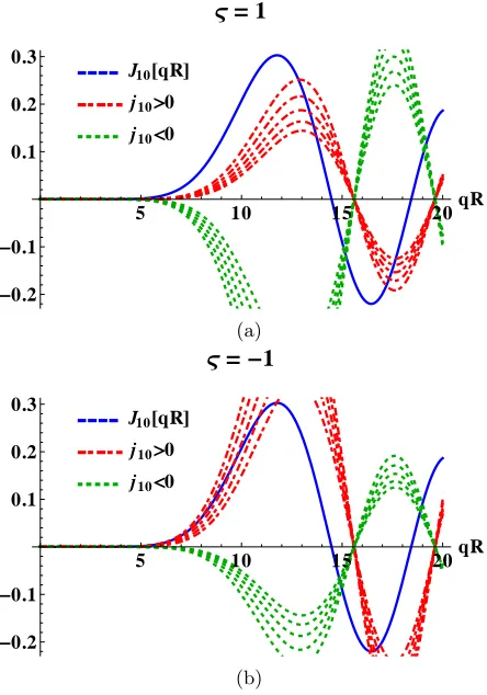
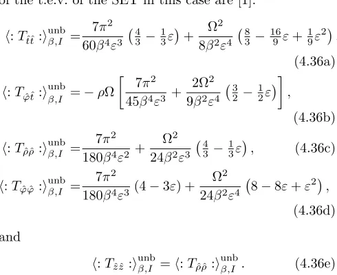
Now consider the lowest value of the transverse momen-tum, qm,1. We have Jm(qm,1R) = jm1Jm+1(qm,1R), in other words, when q = qm,1 the graphs of the func-tionsJm(qR) andjm1Jm+1(qR) intersect. The inequality (3.48) tells thatjm1 <1, so Jm(qm,1R)< Jm+1(qm,1R). Therefore the value ofqm,1Ris in the interval where Jm decreases towards its first zero, after the first zero ofJm0 . Fig. 1(a) illustrates this behaviour. Hence, in this case, we can use the same argument as that given above in the massless case to show that the lowest allowed positive energy obeys ER >e (1−ΩR)(m+ 12). Therefore when
ς= 1 we again haveEE >e 0 for allR≤Ω−1.
In the chiral case (ς =−1), from (3.47),jm` increases as the mass increases andqm,1R approaches the origin, as illustrated in Fig. 1(b). Rearranging Eq. (3.47) as:
q Jm(qR) Jm+1(qR)
=µ+E(µ), (3.49)
where E(µ) = pµ2+q2 is the smallest positive Minkowski energy for a particle of massµand transverse momentumq(i.e. corresponding tok= 0), it can be seen thatqR= 0 is a solution of (3.35) whenµR=m+ 1, by using:
lim z→0z
Jm(z) Jm+1(z)
= 2(m+ 1). (3.50)
If the mass µ increases further, the first root no longer corresponds tojm`>0 (i.e. the root satisfyingqm,`R < ξm,1disappears). In this case, withµR >1 +m, we have ER > m+12 just from the mass contribution to E(µ). Knowing that, by virtue of Eq. (3.45), the same condition is satisfied when µ = 0, it remains to investigate the behaviour of the smallest allowed energyEm,1(µ) forqm,1 betweenµR= 0 andµR=m+ 1.
To this end, let us consider the derivative of Em,1(µ) with respect toµ:
Em,10 (µ) = 1 Em,1(µ)
5 10 15 20qR
-0.2
-0.1
0.1 0.2 0.3
̣=1
j10<0
j10>0
J10@qRD
(a)
5 10 15 20qR
-0.2
-0.1
0.1 0.2 0.3
̣= -1
j10<0
j10>0
J10@qRD
[image:10.612.63.285.54.371.2](b)
FIG. 1. Graphs for finding the first value of the transverse momentum qm,1 allowed by the MIT bag boundary condi-tions for m = 10. The roots of Eq. (3.35) are located at the intersection between the solid line (representingJm(qR)) and the dashed lines (representingJm(qR) multiplied by the right-hand side of Eq. (3.47)). The dashed lines correspond to masses µR = 0,2,4,6,8 and 10, while ς = 1 in (a) and
ς = −1 in (b). The two sets of dashed lines correspond to the sign ofjm`, i.e. the dash-dot lines (red curves, positive for smallqR) correspond tojm`>0 while the dashed lines (green curves, negative for smallqR) represent the casejm`<0.
where the prime denotes differentiation with respect to the argument µ. Since qm,1(µ) decreases as the mass increases,q0m,1(µ)<0 for this range ofµRandEm,10 (µ= 0)<0. The energy reaches a minimum when
qm,1(µ0)q0m,1(µ0) =−µ0. (3.52)
A second expression forEm,10 (µ) can be obtained by tak-ing the derivative of Eq. (3.49) with respect toµ:
q0 Jm(qR) Jm+1(qR)
1 +RJ
0
m(qR) Jm(qR)
−RJ
0
m+1(qR) Jm+1(qR)
= 1 +E0. (3.53) Using Eq. (3.51) to eliminateqm,10 in favour ofEm,1, to-gether with the following properties of the Bessel
func-tions:
Jm0 (z) =−Jm+1(z) + m
zJm(z), Jm+10 (z) =Jm(z)−
m+ 1
z Jm+1(z), (3.54) Eq. (3.53) can be solved to yield:
E0(µ) = µ(2m+ 1)−2µER+E
E(2m+ 1)−2E2R+µ. (3.55) SinceE0(µ) <0 at µ= 0, either Em,1 reaches its min-imum when µR = m+ 1 (in which case qm,1 = 0 and Em,1 = µ = R−1(m+ 1)), or there must be at least one value µ = µ0 between 0 and R−1(m+ 1) where E0(µ0) = 0. At such a point, Eq. (3.55) predicts that the value of the energy would be:
E(µ0)R=
2µ0R 2µ0R−1
(m+12). (3.56) Since E was assumed to be positive, Eq. (3.56) implies thatEcannot be minimized with respect to the mass for µ0R≤ 12. If a stationary point occurs for anyµ0R > 12, the corresponding value of the energy will be greater than R−1(m+12). Since the energy is aboveR−1(m+12) at the endpointsµ= 0 andµ=m+ 1 (where the corresponding value ofq would be 0) and since at its stationary points we also haveE > R−1(m+1
2), we can conclude that the energy will always satisfy:
Em,`R > m+ 1
2, (3.57)
and therefore, using (2.12),
e
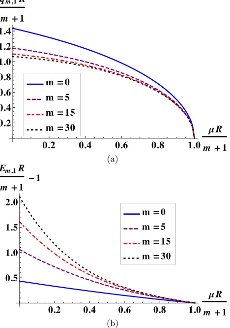
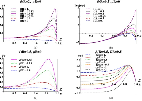
Em,`R >(1−ΩR)(m+12). (3.58) Our numerical experiments confirm Eq. (3.57). Fur-thermore, the energy seems to decrease monotonically towards its minimum value of (m+ 1)/RasµRincreases from 0 tom+ 1, as shown in Fig. 2.
Hence, the MIT bag boundary conditions withς=±1 restrict the energy spectrum such that EE >e 0 for all
values ofµ, k, m and `, as long as the boundary of the cylinder is inside or on the SOL.
3. Normalization
We now turn to the normalization of the MIT modes (3.39). We require these modes to have unit norm with respect to the Dirac inner product (2.30):
hUjMIT, UjMIT0 i=δ(j, j0), (3.59)
whereδ(j, j0) is defined in analogy to Eq. (3.20): δ(j, j0) =δ(kj−kj0)δmj,m
0.2 0.4 0.6 0.8 1.0
ΜR
m+1 0.2
0.4 0.6 0.8 1.0 1.2 1.4
qm,1R
m+1
m=30 m=15
m=5
m=0
(a)
0.2 0.4 0.6 0.8 1.0
ΜR
m+1 0.5
1.0 1.5 2.0 Em,1R
m +1 -1
m=30
m=15 m=5
m=0
[image:11.612.62.296.57.390.2](b)
FIG. 2. The dependence of the smallest allowed transverse momentum (a) and energy (b) in the MIT bag model cor-responding to ς = −1 for µR between 0 and m+ 1 and
m= 0,5,15,30. Thexaxis represents the ratioµR/(m+ 1), normalizing the mass such that for any value ofm, the range of thexaxis is from 0 to 1. The transverse momentumqm,1 and energyEm,1 are divided byR−1(m+ 1). Plot (b) shows the difference Em,1R
m+1 −1 in terms of µR/(m+ 1). The en-ergyEm,1 is monotonically decreasing and has no stationary points for this range of values ofµR.
where, as in the spectral case,θ(EjEj0) ensures thatEj
andEj0 have the same sign. There is no helicity
depen-dence in (3.60) because the MIT modes (3.39) are linear combinations of positive and negative helicity spinors.
The time invariance of the Dirac inner product (3.1), guaranteed to hold in the MIT bag model by Eq. (3.28), ensures that the result of the inner product of modes with different corotating energies (i.e. nonzero ∆Ee=Eej−Eej0)
vanishes. Thus, the following result is obtained:
hUjMIT, UjMIT0 i=
1 4δ(k−k
0)δ
mm0δ``0θ(EE0) ×
CEkm`MIT
2h
(S+ ++S
−
+)I + m+1
2 + (S+
−+S − −)I
−
m+1 2
i
,
(3.61) where the integrals I±m+1
2
were introduced in Eq. (3.21)
and their coefficients are given by:
S+
± =E2+(bEkm`p++p−)2±E2−(bEkm`p−+p+)2, (3.62a)
S±− =E2−(bEkm`p+−p−)2±E2+(bEkm`p−−p+)2, (3.62b)
wherep± are defined in (2.24), E± are defined in (2.29)
and b is given in (3.38). The combinations of S+
± and
S±− occuring in Eq. (3.61) can be evaluated using the following identities:
S±+=4k 2 E2
1±j2 m`
(|ςEE|E+p+jm`−E−p−)2
, (3.63a)
S±−=4k 2 E2
1±j2m`
(|ςEE|E−p+jm`+E+p−)2
, (3.63b)
wherejm`is given by (3.36). Then we have
S+
± +S±−=
8(1±j2 m`) p2
+j2m`+p 2
−
. (3.63c)
Hence, the modes (3.39) are normalized according to Eq. (3.59) if
CjMIT=
1 R|Jm+1(qm,`R)|
×
v u u t
p2
−+p2+j2m` (j2
m`+ 1)(j 2
m`+ 1− 2m+1
qm,`Rjm`)−(j
2 m`−1)
jm`
qm,`R
.
(3.64)
In the massless limit,CMIT
j (3.64) simplifies to:
CMIT j cµ=0=
1
R√2|Jm+1(qm,`R)|
1−jm`(m+
1 2) qm,`R
−
1 2 .
(3.65) The normalization constant CMIT
j (3.64) is invariant under (E, k, m)→(−E,−k,−m−1). The quantitybj, defined in Eq. (3.38), is also invariant under the same transformation. Therefore, using the property (2.33), the relationship between particle and anti-particle spinors satisfying the MIT bag boundary conditions is:
VjMIT= (−1)mj iEj
|Ej|
UMIT, (3.66)
where
= (−Ej,−kj,−mj−1, `j). (3.67)
Since the particle modesUMIT
4. Second quantization
For the remainder of this paper, we shall assume that RΩ ≤ 1 and the boundary is located inside or on the SOL. In this case, we have shown in Sec. III C 2 that EE >e 0 for all fermion field modes satisfying MIT
bag boundary conditions. As discussed in Sec. II C, this means that the rotating and nonrotating Minkowski vacua are the same and second quantization of the field is straightforward. The quantum fermion field is expanded in terms of the normalized modes (3.39, 3.66):
ψ=X j
θ(Ej)
h
UjMITbMITj +VjMITdMITj †i, (3.68)
where j is defined in Eq. (3.41) and the sum over j is defined as:
X
j
≡
∞ X
mj=−∞
∞ X
`j=1
Z ∞
−∞
dkj
X
Ej=±|Ej|
. (3.69)
There is no sum over helicity because the modes (3.39) are linear combinations of positive and negative helicity spinors.
The vacuum for the MIT case,|0MITi, is then defined as that state which is annihilated by the operatorsbMIT
j anddMIT
j :
bMITj |0MITi= 0 =dMITj |0MITi. (3.70) In Sec. IV C, we will calculate expectation values for ther-mal states constructed from|0MITi.
D. Summary
In this section, we have considered a quantum fermion field on rotating Minkowski space-time inside a cylinder of radius R with the axis of the cylinder along the z-axis. We have examined two boundary conditions for the fermion field on the surface of the cylinder: spec-tral [8] and MIT bag [9, 10]. In each case we have stud-ied the quantization condition for the transverse momen-tum, the resulting energy spectrum and the correspond-ing normalized mode solutions. An important conclusion pertaining to the energy spectrum, summarized in sub-sections III B 2 and III C 2 for the spectral and MIT cases, respectively, was that modes withEjEej <0 are excluded from the energy spectrum if the boundary is placed in-side the SOL, that is, RΩ ≤ 1 where Ω is the angular speed about the z-axis. In this case the rotating and nonrotating Minkowski vacua are identical and second quantization of the fermion field is straightforward.
IV. THERMAL EXPECTATION VALUES
In this section, we calculate rigidly-rotating thermal expectation values (t.e.v.s) of the fermion condensate
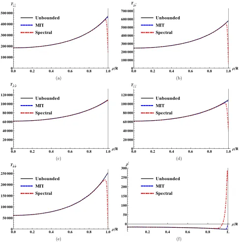
ψψ (FC), parity-violating neutrino charge current Jzν (CC) and stress-energy tensorTµν (SET) for a quantum fermion field inside a cylinder of radiusR, whereRΩ≤1 and the boundary is inside or on the SOL (speed-of-light surface). We use the thermal Hadamard function and the point-splitting method, as outlined in Ref. [19]. The spectral and MIT bag boundary conditions are consid-ered separately. We compare our results with those for rotating fermions on unbounded Minkowski space-time, as discussed in Refs. [1, 3, 7].
For completeness, the main steps for the construction of the thermal Hadamard function, presented in Ref. [19], are summarized below. We start with the Pauli-Jordan (Schwinger) function,
S(x, x0) =h0|
ψ(x), ψ(x0 |0i, (4.1)
whose Fourier transform can be written as:
S(x, x0) =
Z ∞
−∞
dω e−iω∆tc(ω;x,x0), (4.2)
where x is the spatial part of the space-time point x. We note that since
ψ(x), ψ(x0) is proportional to the identity operator, the Schwinger function S(x, x0) (4.1) is state-independent (i.e. evaluates to the same number regardless of the state |0i under consideration). The Fourier coefficients c(ω;x,x0) can be used to compute the thermal Hadamard function at inverse temperature β:
Sβ(1)(x, x0) =
Z ∞
−∞
dω e−iω∆tc(ω;x,x0) tanhβω
2 . (4.3)
The thermal Hadamard functionS(1)β (x, x0) (4.3) is
inde-pendent of the initial choice of vacuum|0iin (4.1). Since we consider only the case where the boundary is inside the SOL, as discussed in Secs. II C, III B 4, III C 4, the rotating and nonrotating Minkowski vacua inside the cylinder are identical for each set of boundary condi-tions. However, the two vacua for the different bound-ary conditions, namely|0spi(spectral) and|0MITi(MIT) are not the same. In this section, we compute rigidly-rotating t.e.v.s with respect to the|0spiand|0MITi vac-uum states, using the difference ∆Sβ(1)(x, x0) between the
thermal Hadamard functionSβ(1)(x, x0) (4.3) and its vac-uum counterpart, defined as:
S(1)(x, x0) =h0∗|
ψ(x), ψ(x0)
|0∗i, (4.4)
A. Thermal Hadamard function
Using the notation in Eq. (2.10), the fermion field op-erator can be written as:
ψ(x) = 1 2π
X
j θ(Ej)
h
e−iEejt+ikjzC
juj(x)bj
+eiEejt−ikjzC∗
jvj(x)d†j
i
, (4.5) where the sum over j, the normalization constants Cj, the four-spinors uj and their charge conjugates vj pend on the boundary conditions employed, and are de-scribed in detail in Sec. III. The corotating energy Eej and the Minkowski energyEj are related by Eq. (2.12). The Schwinger function (4.1) takes the form:
S(x, x0) =X j
θ(Ej)
Uj(x)⊗Uj(x0) +Vj(x)⊗Vj(x0)
,
(4.6) where ⊗ denotes an outer product, theUj are particle modes and the Vj are anti-particle modes. The expres-sion (4.6) is valid irrespective of the state in which it is evaluated [19]. Thus, the Fourier coefficients of the Schwinger function take the form:
c(ω;x,x0) =X j
|Cj| 2
θ(Ej) 4π2
×hδ(ω−Eej)eikj∆zuj(x)⊗uj(x0) +δ(ω+Eej)e−ikj∆zvj(x)⊗vj(x0)
i
, (4.7)
where ∆z =z−z0. From these Fourier coefficients, the thermal Hadamard function (4.3) can be derived:
Sβ(1)(x, x0) =X j
θ(Ej) tanh βEej
2
×
Uj(x)⊗Uj(x0)−Vj(x)⊗Vj(x0). (4.8) Subtracting the vacuum Hadamard function (4.4) from the above thermal Hadamard function gives:
∆S(1)β (x, x0) =−X
j wj
×
Uj(x)⊗Uj(x0)−Vj(x)⊗Vj(x0), (4.9) where the thermal factorwj takes the form:
wj=
2θ(Ej) eβEej+ 1
. (4.10)
In (4.10), the step function θ(Ej) ensures that the sum over j in Eq. (4.9) runs only over positive Minkowski energies (i.e.Ej >0).
In this section we calculate the (rigidly-rotating) t.e.v.s for the fermion condensate (FC)h:ψψ:i∗β, charge current
h:Jαˆ:i∗βand stress-energy tensor (SET)h:Tαˆˆσ :i∗β, where all components are with respect to the tetrad (2.2). The notation h:O:i∗β, for an operator O, indicates that we are considering t.e.v.s relative to the vacuum state (ei-ther|0spior|0MITias applicable). The superscript∗will
be either sp or MIT depending on which boundary con-ditions we are considering. For the rest of this section, all expectation values will be for rotating thermal states, relative to the appropriate (bounded) vacuum state. We will consider expectation values in the bounded vacuum state relative to the unbounded Minkowski vacuum state in Sec. V.
The t.e.v.s are calculated from the difference (4.9) be-tween the thermal Hadamard function and the vacuum Hadamard function, as follows:
h:ψψ:i∗β=−1
2xlim0→xtr h
∆Sβ(1)(x, x0)i, (4.11a)
h:Jαˆ :i∗β=−1
2xlim0→xtr h
γαˆ∆Sβ(1)(x, x0)i, (4.11b)
h:Tαˆˆσ :i∗β= i 4xlim0→xtr
h
γ( ˆαDˆσ)∆S (1) β (x, x
0)
−∆Sβ(1)(x, x0)←D−(ˆσγα)ˆ
. (4.11c)
It will turn out, in Secs. IV B 2 and IV C 2, that the expectation value (4.11b) for the charge current vanishes identically for both spectral and MIT bag boundary con-ditions. We will therefore also consider the charge cur-rent for fermions of negative chirality only. It has been remarked by Vilenkin [7] that the restriction of the par-ticle spectrum to fermions of negative chirality induces a nonvanishing charge current anti-parallel to the rotation vectorΩ. Since these particles are traditionally called (in the massless case) neutrinos, we will use the term neu-trino charge current (and abbreviate this to CC) for this quantity. The t.e.v.s of the CCJανˆof particles of negative chirality can be calculated using:
h:Jανˆ :i
∗
β=− 1 2xlim0→xtr
γαˆ1−γ 5
2 ∆S
(1) β (x, x
0)
.
(4.11d) Here (1−γ5)/2 projects onto the space of modes of nega-tive chirality with the help of the matrixγ5=iγˆ0γˆ1γˆ2γˆ3, which in the Dirac representation has the form [13]:
γ5=
0 1 1 0
. (4.12)
We now turn to the computation of the t.e.v.s (4.11), considering the spectral and MIT bag boundary condi-tions separately. In each case, we first construct the ther-mal Hadamard function before computing the t.e.v.s and examining their properties.
B. Spectral boundary conditions
be-tween the thermal and vacuum Hadamard functions (4.9) can be written as:
∆Sβ(1)(x, x0) =−X
j
C
sp j
2 4π2 e
−iEej∆t+ikj∆z(w
j−w)Mjλ, (4.13) whereEejis the corotating energy, ∆t=t−t0, ∆z=z−z0 and the normalization constantCjsp ≡ Cλj,sp
Ejkjmj`j is given
in Eq. (3.22). The sum overjcan be found in (3.26). The thermal factors wj and w are given by (4.10) with the indicesjandin Eqs. (3.15) and (3.24) respectively. The matrixMjλ ≡Mjλ(x, x0) =uλj
Ejkjmj`j(x)⊗u
λj
Ejkjmj`j(x
0)
is given explicitly by:
Mjλ= 1 2
E2
+ −2λE|E|E+E−
2λE
|E|E+E− −E2− !
⊗hφj(x)⊗φ†j(x
0)i,
(4.14) whereE±are given in (2.29) and the spinorsφj in (2.23). In (4.14), the first occurrence of⊗has the meaning of a Kronecker product of two 2×2 matrices, i.e.:
a11 a12 a21 a22
⊗B=
a11B a12B a21B a22B
. (4.15)
In other words, the outer productφj(x)⊗φ†j(x0) is to be copied into each of the four matrix elements to the left of the Kronecker⊗sign, thus producing a 4×4 matrix.
Introducing the following notation:
Mj≡
X
λj=±1/2
Mjλ=1 2
Mup
j −M
×
j Mj× −Mdown
j
, (4.16)
the following expressions can be found for the 2×2 matri-ces introduced on the right-hand-side of (4.16), by using the explicit form (2.23) of theφj spinors:
Mjup=E2+
1 0 0 1
◦ Mj,
Mjdown=E2−
1 0 0 1
◦ Mj,
Mj×=1 E
k q q −k
◦ Mj. (4.17)
In (4.17), the Hadamard (Schur) product symbol ◦ has been used for the element-wise product of two matrices of the same size, defined for two 2×2 matricesA,B as:
A◦B=
a11b11 a12b12 a21b21 a22b22
. (4.18)
The matrix Mj on the right of the Hadamard product symbol◦ in (4.17) is defined as:
Mj=
JmJmeim∆ϕ −iJmJm+1ei(m+1)∆ϕ−iϕ iJm+1Jmeim∆ϕ+iϕ Jm+1Jm+1ei(m+1)∆ϕ
,
(4.19)
where ∆ϕ=ϕ−ϕ0 and the arguments of the first and second Bessel functions in the products above areqρand qρ0, respectively, e.g.JmJm+1≡Jm(qρ)Jm+1(qρ0).
For the purpose of computing t.e.v.s, it is advantageous to writeMj (4.16) as:
2Mj = 1
2I2⊗(M up j −M
down j ) +1
2σ3⊗(M up j +M
down j ) +
0 −1 1 0
⊗Mj×, (4.20)
whereI2is the 2×2 identity matrix and the Pauli matrix σ3can be found in Eq. (2.5). Thus, the following form is obtained forMj:
Mj=
µ 2EI2+
1 2σ3
⊗
1 0 0 1
◦ Mj
+ 1 2E
0 −1 1 0
⊗
k q q −k
◦ Mj
. (4.21)
Having computed above the explicit form ofMj appear-ing in Eq. (4.13), t.e.v.s can now be calculated, as de-scribed in the following sections.
1. Fermion condensate
The t.e.v. of the fermion condensate (FC) h:ψψ:ispβ is computed from the difference between the thermal and vacuum Hadamard functions (4.13) using (4.11a). Look-ing at Eq. (4.21), it is clear that only the first term (the one involvingI2on the left of the direct product sign⊗) contributes, giving:
h:ψψ:ispβ =X j
C
sp j
2
8π2 (wj−w) µ Ej
Jm+(qρ), (4.22)
where the notationJ+
m(z) is the same as in Ref. [1]: Jm±(z) =Jm2(z)±Jm+12 (z),
Jm×(z) =2Jm(z)Jm+1(z). (4.23) It is convenient to express the sum overj as a sum over positive energies:
h:ψψ:ispβ =
∞ X
m=0
∞ X
`=1
Z ∞
0
µ dk Eπ2R2
w(E) +e w(E)
J2 m+1(qR)
Jm+(qρ), (4.24) where we have used (3.22) for the normalisation constants
Cjsp and the thermal weight factorw(x) is:
w(x) = 2
eβx+ 1, (4.25)
while its argumentsEe andE are defined as:
e
0.2 0.4 0.6 0.8 1.0 Ρ
R
0.002 0.004 0.006 0.008 0.010
ΨΨΜ
ΒR=2,ΜR=0
WR=0. WR=0.5 WR=0.65 WR=0.8 WR=0.9 WR=1.
0.2 0.4 0.6 0.8 1.0 Ρ
R
0.5 1.0 1.5 2.0 2.5
ΨΨΜ
ΒR=0.5,ΜR=0
WR=0. WR=0.5 WR=0.65 WR=0.8 WR=0.9 WR=1.
(a) (b)
0.2 0.4 0.6 0.8 1.0 Ρ
R
0.05 0.10 0.15 0.20 0.25 0.30
ΨΨΜ
WR=0.5,ΜR=0
ΒR=1.4 ΒR=1. ΒR=0.75 ΒR=0.65
0.2 0.4 0.6 0.8 1.0 Ρ
R
0 20 40 60 80
ΨΨΜ
ΒR=0.05,WR=0.5
ΜR=100. ΜR=50. ΜR=20. ΜR=0.
Un boun ded
[image:15.612.79.510.54.367.2](c) (d)
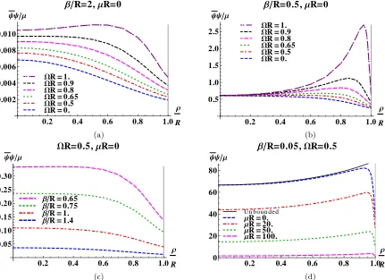
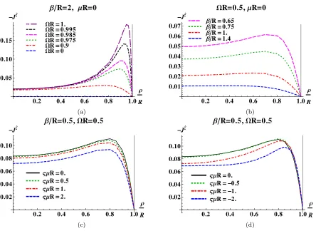
FIG. 3. Thermal expectation values (t.e.v.s) of the fermion condensate (FC)h:ψψ:ispβ (4.24) for spectral boundary conditions divided by the fermion massµ, as a function of the scaled radial coordinateρ/R, so that the boundary of the cylinder is at
ρ/R= 1. (a) Massless fermionsµ= 0, fixed inverse temperatureβ= 2Rand various values of the angular speed Ω. (b) Massless fermionsµ= 0, fixed inverse temperatureβ= 0.5Rand various values of the angular speed Ω. (c) Massless fermionsµ= 0, fixed angular speed Ω = 0.5/R and various values of the inverse temperature β. (d) Fixed inverse temperatureβ = 0.05R, fixed angular speed Ω = 0.5/Rand various values of the fermion massµ. The solid curve in (d) shows the t.e.v. of the FC for massless fermions in the unbounded case, given in Eq. (4.27), for comparison.
Thus, in the spectral model, the t.e.v. of the FC van-ishes for massless fermions withµ= 0. In Fig. 3 we have therefore plottedµ−1h:ψψ:ispβ to facilitate comparisons between the t.e.v.s for different values of the mass µ. It can be seen from Fig. 3 that the t.e.v. of the FC is pos-itive everywhere, including on the boundary, where its value is finite. This is true for all R provided that the boundary of the cylinder is either inside or on the SOL. In Fig. 3 (a) and (b), we have fixed the inverse temperature β and the fermion mass µ = 0, and show the t.e.v.s of µ−1h:ψψ:isp
β for various values of the angular speed Ω. The t.e.v. of the FC increases for each fixed value ofρas ΩRincreases. This is particularly marked in the higher-temperature plot (b). When ΩR= 1 and the boundary is on the SOL, the FC increases rapidly as we move away from the axis of rotation, with a large peak just inside the boundary. However, even in this case, the FC is finite on the boundary. In (c) we have fixed the angular speed Ω and again consider massless fermionsµ= 0, varying the inverse temperatureβ. As expected, the t.e.v.s decrease asβincreases and the temperature decreases. Finally, in
(d) we fix the inverse temperatureβand angular speed Ω and vary the fermion massµ. We see thatµ−1h:ψψ:ispβ
decreases asµincreases.
For comparison, in Fig. 3(d) we also plot the t.e.v. of the FC corresponding to the massless unbounded case [1]:
1
µh: [ψψ] :i unb β,I
µ=0
=− 1
2. Neutrino charge current
Next, we consider the t.e.v. of the charge current op-eratorh:Jαˆ:isp
β, defined in (4.11b). It is straightforward to see that the t.e.v.s of all the components of h:Jαˆ :isp β vanish. This is because the expression forh:Jαˆ :isp
β anal-ogous to (4.22) contains a summand which is odd under either m → −m−1 (for α ∈ {t, ρ, ϕ}) or k → −k (for α=z). To illustrate this point, let us consider the time component:
h:Jˆt:ispβ =−X
j
(wj−w)
C
sp j
2 8π2 J
+
m(qρ), (4.28)
where the various quantities are defined in (3.22, 4.10, 4.23). After restricting the energy to positive values, Eq. (4.28) reduces to:
h:Jˆt:ispβ =
∞ X
m=−∞ ∞ X
`=1
Z ∞
−∞
dk 2π2R2
w(E)e −w(E)
Jm+12 (qR) J + m(qρ),
(4.29) where the thermal weight factors and their arguments are given in (4.25, 4.26). Since the summand in (4.29) is odd with respect to m → −m−1, we can conclude thath:Jˆt:isp
β = 0. Similar arguments apply to the other components ofh:Jαˆ:ispβ.
We therefore consider the neutrino charge current (CC), whose t.e.v. is given by (4.11d). While the t, ρ andϕcomponents of the CC vanish, thezcomponent is nonzero (in accordance with [7]):
h:Jzνˆ:ispβ =−
∞ X
m=0
∞ X
`=1
Z ∞
0 dk 2π2R2
w(E)e −w(E)
J2 m+1(qR)
Jm−(qρ), (4.30a) whereJ−
m(qρ) is defined in (4.23).
In Fig. 4 we plot the t.e.v. (4.30a) for a range of values of the fermion massµ, inverse temperatureβand angular speed Ω. For all values of the parameters we studied, it can be seen in Fig. 4 that the t.e.v. of the CC changes sign from negative on the axis of rotation ρ = 0 to positive on the boundaryρ=R. This can be explicitly checked by considering the value ofh:Jˆzν:ispβ on the rotation axis ρ= 0,
h:Jzνˆ:ispβk
ρ=0 =−
∞ X
`=1
Z ∞
0
dk 2π2R2J2
1(qR)
×
w
E−Ω
2
−w
E+Ω 2
<0, (4.30b)
and on the boundary ρ = R (recall that Ee and E are
given in (4.26)):
h:Jzνˆ:ispβk
ρ=R=
∞ X
m=0
∞ X
`=1
Z ∞
0 dk
2π2R2[w(E)e −w(E)]>0. (4.30c)
0.2 0.4 0.6 0.8 1.0
Ρ
R
-0.010 -0.005 0.005 0.010 Jz`
ΒR=2,ΜR=0
WR=0. WR=0.5
WR=0.65
WR=0.8 WR=0.9 WR=1.
(a)
0.2 0.4 0.6 0.8 1.0
Ρ
R
-0.10 -0.05 0.05 0.10 0.15 Jz`
WR=0.5,ΜR=0
ΒR=1.4 ΒR=1. ΒR=0.75 ΒR=0.65
(b)
0.96 0.98 1.
Ρ
R 0
100 200 300 400 500 600 Jz`
ΒR=0.05,WR=0.5
Un boun ded
ΜR=100. ΜR=50. ΜR=20. ΜR=0.
[image:16.612.332.537.53.487.2](c)
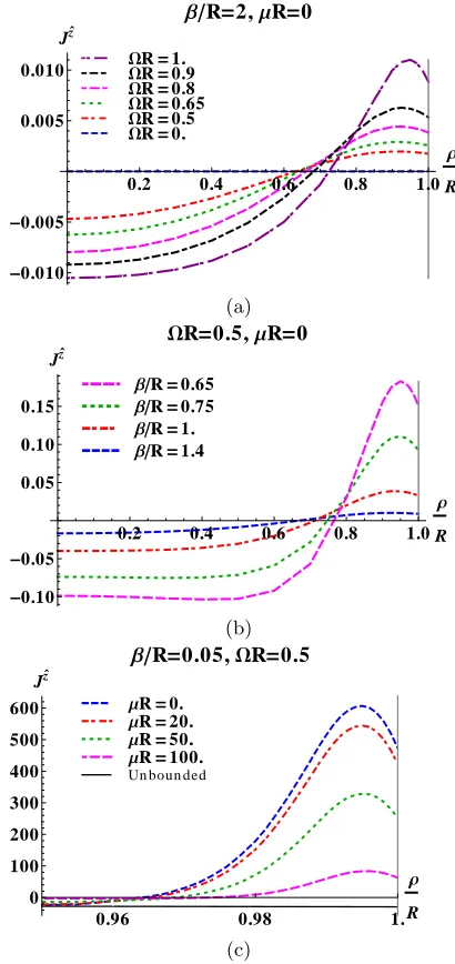
FIG. 4. Thermal expectation values (t.e.v.s) of the neutrino charge current (CC)h:Jαˆν:ispβ (4.30a) for spectral boundary conditions, as a function of the scaled radial coordinateρ/R, so that the boundary of the cylinder is atρ/R= 1. (a) Mass-less fermionsµ = 0, fixed inverse temperatureβ = 2R and various values of the angular speed Ω. (b) Massless fermions
µ= 0, fixed angular speed Ω = 0.5/R and various values of the inverse temperatureβ. (c) Zoom of the region close to the boundary at fixed inverse temperatureβ= 0.05R, fixed angular speed Ω = 0.5/R and various values of the fermion massµ. The solid curve in (c) shows the t.e.v. of the CC for massless fermions in the unbounded case, given in Eq. (4.31), for comparison.
As the angular speed Ω or temperature β−1 increase, the t.e.v.h:Jzˆ
ν :i sp
β decreases on the axis of rotation and increases on the boundary. It remains finite everywhere inside and on the boundary. In Fig. 4 (a) we see that
h:Jˆz ν:i
sp
is also the case on unbounded Minkowski space-time [1]. As the fermion massµincreases,h:Jzˆ
ν :i sp
β also decreases close to the boundary. Fig. 4 (c) also shows the t.e.v. of the CC for the massless unbounded case, which is given by [1]:
h:Jzˆ:iunbβ,I =− Ω
12β2ε2. (4.31) Close to the boundary, h:Jzνˆ:i
sp
β changes sign and in-creases to values which are an order of magnitude higher than the absolute value of h:Jzˆ:iunb
β,I, which is negative everywhere. In Fig. 4 (c), note thath:Jˆz:iunbβ,I is not con-stant, as it might appear. It changes only by a small amount in the region shown, whereas h:Jzˆ
ν :i sp
β changes very rapidly in this region.
3. Stress-energy tensor
The t.e.v. of the stress-energy tensor (SET)h:Tαˆˆσ :i sp β with respect to the tetrad (2.2) can be calculated using
the formula (4.11c), with the difference between the ther-mal and vacuum Hadamard functions given by (4.13). By construction, the action of iDˆt on e−
iEejtM
j (with the matrixMj given in (4.14)) gives the energyEj:
iDˆte− iEejtM
j=Eje−iEejtMj, (4.32)
while for the derivatives with respect to ρ and ϕ, the inner structure (4.19) of theMj matrix must be taken into account. Using the quantities defined in (4.23, 4.25, 4.26), together with the relation
Jm+10 (z)Jm(z)−Jm0 (z)Jm+1(z) =Jm+(z)− m+1
2 z J
×
m(z), (4.33) we find the following expressions for the components of the t.e.v.h:Tαˆˆσ:i
sp
β relative to the tetrad (2.2):
h:Tˆtˆt:i sp β =
∞ X
m=0
∞ X
`=1
Z ∞
0 E dk π2R2
w(E) +e w(E)
J2 m+1(qR)
Jm+(qρ), (4.34a)
h:Tρˆˆρ:i sp β =
∞ X
m=0
∞ X
`=1
Z ∞
0
q2dk Eπ2R2
w(E) +e w(E)
J2 m+1(qR)
Jm+(qρ)−m+
1 2 qR J
×
m(qρ)
, (4.34b)
h:Tϕˆϕˆ:i sp β =
∞ X
m=0
∞ X
`=1
Z ∞
0
q dk ρEπ2R2
w(E) +e w(E)
J2 m+1(qR)
(m+1 2)J
×
m(qρ), (4.34c)
h:Tzˆˆz:i sp β =
∞ X
m=0
∞ X
`=1
Z ∞
0
k2dk Eπ2R2
w(E) +e w(E)
J2 m+1(qR)
Jm+(qρ), (4.34d)
h:Tˆtˆϕ:i sp β =−
∞ X
m=0
∞ X
`=1
Z ∞
0 dk ρπ2R2
w(E)e −w(E)
J2 m+1(qR)
(m+12)Jm+(qρ)−12J
−
m(qρ) +qρJm×(qρ)
. (4.34e)
Eqs. (4.34) can be used to check the identity:
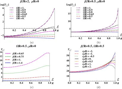
h:Tαˆαˆ :iβ =−µh:ψψ:iβ. (4.35) In Fig. 5 we have plotted the t.e.v. h:Tˆttˆ:i
sp
β (4.34a) for a range of values of the inverse temperatureβ, angu-lar speed Ω and fermion mass µ. Other components of (4.34) are discussed in Sec. IV D. As was observed earlier for the FC and CC, if the angular speed Ω or tempera-tureβ−1 increase with the other parameters fixed, then the t.e.v.h:Ttˆˆt:i
sp
β also increases. It is finite everywhere inside and on the boundary, including in the case where ΩR= 1 and the boundary is on the SOL. When ΩR= 1, in Figs. 5 (a) and (b), we see a large peak in h:Tˆtˆt:i
sp β close to the boundary. Fig. 5 (d) shows that h:Tˆtˆt:i
sp β