.
White Rose Research Online URL for this paper: http://eprints.whiterose.ac.uk/1315/
Article:
Humphries, M.D., Gurney, K. and Prescott, T.J. (2006) The brainstem reticular formation is a small-world, not scale-free, network. Proceedings of the Royal Society B: Biological Sciences, 273 (1585). pp. 503-511. ISSN 1471-2954
https://doi.org/10.1098/rspb.2005.3354
[email protected] https://eprints.whiterose.ac.uk/
Reuse
Unless indicated otherwise, fulltext items are protected by copyright with all rights reserved. The copyright exception in section 29 of the Copyright, Designs and Patents Act 1988 allows the making of a single copy solely for the purpose of non-commercial research or private study within the limits of fair dealing. The publisher or other rights-holder may allow further reproduction and re-use of this version - refer to the White Rose Research Online record for this item. Where records identify the publisher as the copyright holder, users can verify any specific terms of use on the publisher’s website.
Takedown
If you consider content in White Rose Research Online to be in breach of UK law, please notify us by
Electronic Appendices for: The brainstem reticular formation is a
small-world, not scale-free, network
M. D. Humphries, K. Gurney, T. J. Prescott
Address: Adaptive Behaviour Research Group, Department of Psychology, University of Sheffield, Sheffield. S10 2TP. UK
Electronic Appendix A provides a summary of the functional roles of nuclei within the reticular formation other than the medial structures which are the focus of the main text.
Electronic Appendix B derives the expected number of synaptic connections for the pro-jection and inter-neurons given a parameter set. These values form the basis of the pruning model algorithm.
Electronic Appendix C reports further values of interest from the small-world analysis of the anatomical models.
Electronic Appendix D details the results of fitting curves to the probability distribution functions corresponding to the cumulative degree distributions fits reported in the main text.
Electronic Appendix E considers the plausibility of ever finding a true scale-free network within neural tissue.
Electronic Appendix F discusses the implications of bounds from existing biological data on the parameter-dependency of the small-world topology.
A
Neuroanatomy: Functional roles of the constituent
fields and nuclei
B
Expected numbers of connections in the
anatomi-cal models
The pruning model algorithm runs until it reaches a target value of remaining number of synapses, which is computed according to the expected synapse totals for a given target parameter set: tp is the target value of P(p) and tl is the target value of P(l). Expected synapse total E(Ns) =E(Np) +E(Nl) is the sum of expected totals of projection E(Ne) and inter-neuron E(Nl) originating synapses. For both collateral variants, E(Nl) is the same:
E(Nl) = n−(n−1)Nctl, (1)
where n− =n(1−ρ) is the number of inter-neurons in a cluster (remembering that n is
the total number of neurons in a cluster).
As there are two collateral variants, there are two definitions of E(Np). For the spatially uniform variant, this is straightforward:
E(Np) =Nc np (Nc−1)P(c)tp n, (2)
where np = n ρ is the number of projection neurons in a cluster. However, for the
distance-dependent variant, the expected number of cluster contacts per projection neu-ron is dependent on the position of its parent cluster. Thus, we know that for a given projection neuron in cluster c, its expected number of cluster contactsE(Nc
q) is
E(Nc q) = 2
Ãdmin X
i=1
i−a !
+
dmax
X
i=dmin+1
i−a (3)
where dmin and dmax are
dmin = min(Nc−c,(Nc−1)−(Nc−c)) (4)
dmax = max(Nc−c,(Nc−1)−(Nc−c)) (5)
in words, dmin is the minimum and dmax is the maximum number of intervening clusters to either end of the model from cluster c. Thus, E(Np) for the distance-dependent model is given by
E(Np) =np
ÃNc X
c=1
E(Nqc)
!
tp n. (6)
C
Small-world topologies of the stochastic model
Table 1: First six parameter combinations ordered by maximum S for spatially-uniform (U) and distance-dependent (D) collateral probability models.
ρ P(l) P(p) Su
max Smaxd
0.7 0.9 0.1 4.6612 10.0513 0.7 0.5 0.1 3.1197 6.9934 0.8 0.9 0.1 2.6488 5.8910 0.8 0.5 0.1 1.9645 4.2939 0.7 0.9 0.5 1.6500 3.4214 0.9 0.9 0.1 1.4694 3.0680
D
Degree distribution curve-fitting
We used the curve equations and initial conditions given in Table 2. As is common prac-tice, these were fitted to the invertedcumulative degree distribution 1−F(β) (we retain the F(β) term in the main text to avoid unnecessary confusion) using the MatLab func-tion lsqcurvefit. The inverted distribufunc-tion was used in line with previous work (Amaral, Scala, Barthelemy, & Stanley, 2000; Strogatz, 2001): this ensures, among other things, thatτ >0 as required. Before fitting the exponential curve, all values in the data vectorx
were shifted by the first element(x=x−x1) so that thex1 = 0, and thus the exponential
fit would start at 1.
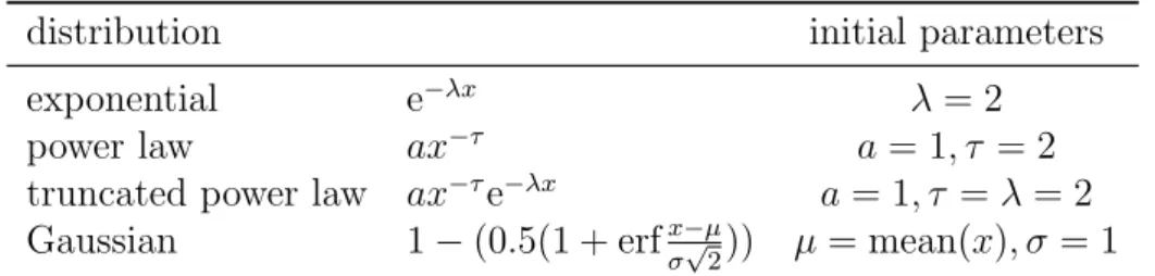
Table 2: Fitted curves to the degree distribution and initial search parameters. Data point isx.
distribution initial parameters
exponential e−λx λ = 2
power law ax−τ a= 1, τ = 2
truncated power law ax−τe−λx a= 1, τ =λ= 2
Gaussian 1−(0.5(1 + erfx−µ
σ√2)) µ= mean(x), σ= 1
The curve-fits were quantitatively compared using Akaike’s Information Criterion (cor-rected). The basic form is calculated according to
AIC =Nln
µ
SS N
+ 2K (7)
where N is the number of data points, SS is the sum-of-squares resulting from the curve fit, andK is the number of parameters in the curve plus one (so, for example, K = 2 for the exponential curve). The corrected version adds a term to account for situations in which N →K:
AICc=AIC+2K(K+ 1)
N −K −1. (8)
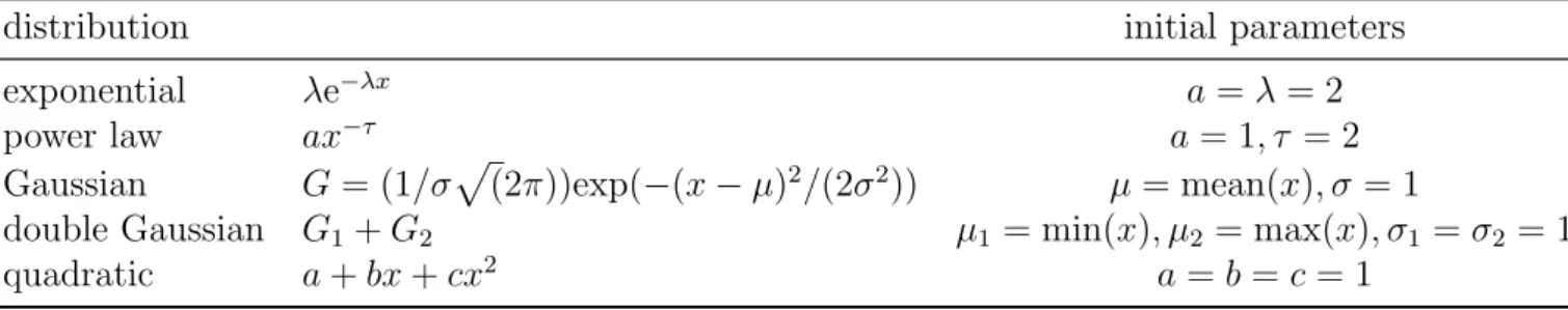
curve family used included exponential, Gaussian, double Gaussian, quadratic, and power law fits (see Table 3). A quadratic fit was included to fitP(β) that the other curves could not.
Table 3: Fitted curves to the degree distribution P(β) and initial search parameters. G1
and G2 refer to separately parameterised Gaussians G.
distribution initial parameters
exponential λe−λx a=λ= 2
power law ax−τ a= 1, τ = 2
Gaussian G= (1/σp
(2π))exp(−(x−µ)2
/(2σ2
)) µ= mean(x), σ= 1
double Gaussian G1+G2 µ1 = min(x), µ2 = max(x), σ1 =σ2 = 1
quadratic a+bx+cx2
a=b=c= 1
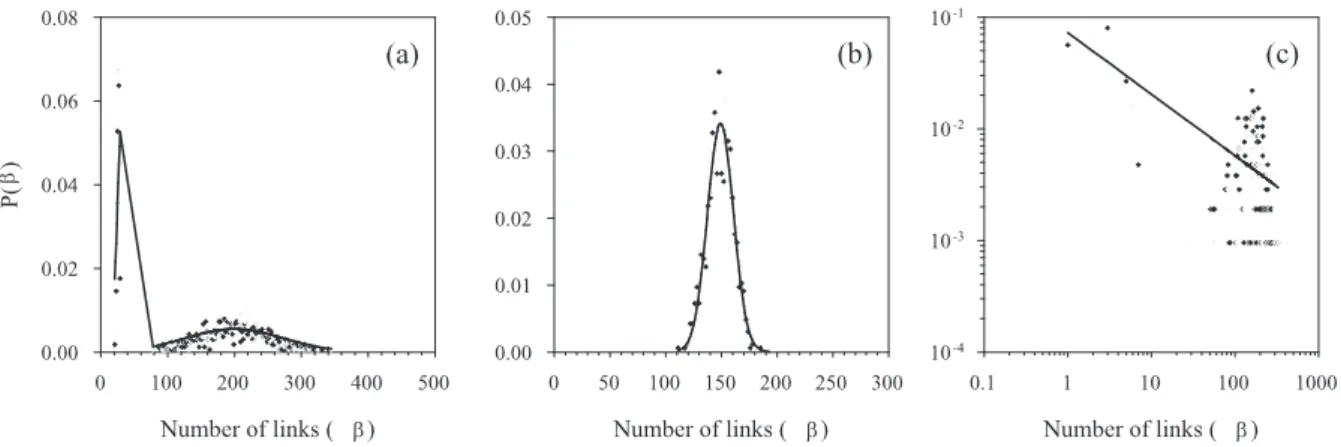
Most of the curve fits were Gaussian or double Gaussian (Table 4) - examples are shown in Figure 1. The double Gaussian fits corresponded to the cumulative degree distributions F(β) poorly fitted by the tested curves, as illustrated in the main text. There is little evidence to suggest that a Gaussian-based distribution of connectivity is not to be expected for neural networks, but we acknowledge that the work on large-scale distributions of axonal or synaptic connectivity is sparse. The observed bimodal (double Gaussian) distributions are due to the different distributions of connectivity for each of the two neuron classes (inter- and projection-neurons). Numerous power law best-fits to P(β) were found, which taken at face value would imply the presence of a scale-free topology. However, the corresponding distributions were not characteristically heavy-tailed (example in Figure 1c) and the corresponding F(β) were best-fit by a Gaussian. We use this result to sound a cautionary note to the reader: despite the generally used, loose definition of a scale-free network, a power-law best fit to a degree distribution is not sufficient evidence to conclude that a network is scale-free (see Li, Alderson, Tanaka, Doyle, and Willinger (2004) for a more rigorous treatment).
Table 4: Percentage best-fit of each curve-type to the P(β) of input, output, and undi-rected links in the spatially-uniform and distance-dependent collateral versions of the stochastic model.
spatially-uniform distance-dependent Curve type inputs outputs undirected inputs outputs undirected
exponential 0.0 2.0 0.0 0.0 0.5 0.0
power law 0.0 22.2 11.4 0.0 20.7 0.0
Gaussian 99.6 24.4 50.4 98.1 26.4 73.8 double Gaussian 0.4 46.9 11.6 1.9 42.0 1.0
quadratic 0.0 4.5 26.6 0.0 10.4 25.2
Figure 1: Best-fit curves to degree distribution P(β), all from the stochastic model. (a) An example of a double Gaussian fit to an output distribution, suggesting the presence of two independent populations within the model. The double Gaussian fits to P(β) seem to correspond to the poorly fitting curves of F(β), as illustrated in the main text. (b) A Gaussian fit to an input distribution from the distance-dependent collateral model - again the dominant best-fit of the tested model curves. (c) Log-log plot showing that the output distribution from the same model instantiation as (b) was best-fit by a power-law. The fit is evidently poor, and the corresponding F(β) was best-fit by a Gaussian. Nevertheless, the input and output distributions of this particular model differ considerably.
based on the quantitative fit results alone, some output P(β) were best fit by different curves to the corresponding input and undirected distributions. Compare the input and output distributions of Figure 1b, c - these are taken from the same instantiation of the spatially-uniform collateral version of the stochastic model. They clearly show that the
P(β)s are different (as are the corresponding F(β)s). As noted by Newman, Strogatz, and Watts (2001) input and output degree distributions of networks are often assumed to be correlated, but there is no a priori requirement that this is the necessary. A ran-domly chosen node in a network has probabilitypij that it has a particular in-degreeiand out-degree j: if the underlying physical process that generates the connection between nodes is independent of the input-output relationship (if the number of links into a node does not effect the number of links coming out, and vice-versa) then the separate distrib-utions are independent and therefore pij =pipj. This in turn would imply that that the undirected distribution would tend towards a Gaussian (or multiple Gaussian). Thus, in general it is possible that input and output degree distributions are not the same, and therefore that a network could be scale-free in one direction only.
E
Power-law degree distributions in neural tissue
a set period, and “cost”, where a node’s ability to support links is physically limited. Both properties apply to neural network development: initial axonal growth and synapse formation is time-limited; the quantity of connections a neuron can develop and sustain is physically limited by the metabolic cost of development, maintenance, and signalling (Cline, 2003; Laughlin & Sejnowski, 2003). The intriguing parallels suggest that it is possible a truncated scale-free topology exists within the nervous system of some species - at some level of neural organisation (neuronal, areal, and so on) - and thus it was not improbable that the medial RF had such a topology.
It is an open question as to whether or not a scale-free network can be developed within neural tissue. The limitations of neural development noted above would suggest that only partially scale-free topologies would be possible. Moreover, although the existence of super-connected hubs would make neural tissue more resistant to random damage - by maintaining network connectivity - the death of such neurons would be catastrophic, and any targeted disease would be highly effective. Such neurons or neuron populations (in particular) should be revealed by systematic anterograde or retrograde staining studies, due to the sheer number of connections they maintain, and would thus be amenable to discovery. On the one hand, as it appears that no such super-connected neurons are reported in the neuroscience literature, it is tempting to conclude that the characteristic hubs of scale-free networks do not exist in neural tissue. On the other hand, given the minute proportion of neurons stained in a typical study compared to the amount in the originating structure, the sampling bias that results in only certain neuron classes being stained within a structure, and the inconsistent uptake of the staining agent, it is possible that either: (a) there has been insufficient sampling to consistently reveal super-connected neurons or (b) that most reported stained neuronsaresuper-connected, which is why they stained consistently in the first place.
F
Dependence of the small-world topology on
con-nection probabilities
The extent to which the medial RF conforms to a small-world topology is partly dependent upon the determination of synaptic connection probabilities (we discuss its dependence on the type of axon collateral distribution and on the validity of the anatomical models in the main text). There are no existing direct estimates of connection probabilities for the medial RF. Data from mouse cortex (Schuz, 1995) and the neural network of C. elegans (Albert & Barabasi, 2002) suggests that the probability of connection between any randomly chosen pair of neurons is p ≤ 0.1 and therefore P(p), P(l)≤ 0.1. If these probabilities were applicable to the medial RF, they would rule out a small-world topology if the combination of stochastic anatomical model and spatially-uniform collaterals were verified (see Figure 2, main text).
However, extrapolating from these unrelated instances is probably unsafe. The di-mensions of the projection neuron dendritic tree suggests, rather, that any axon collateral terminating in a cluster will contact the majority of projection neurons there, and thus
are GABAergic, and putative inter-neurons, but∼45% of the synapses on a giant neuron are GABAergic with no other main afferent GABAergic source, suggesting that the in-terneurons are proportionally more densely connected within a cluster than the incoming projection neurons collaterals. Thus, P(l) > P(p), as required for the most small-world like combinations of the stochastic model - the pruning model would, of course, also have a small-world topology if this relationship held.
References
Aghajanian, G. K., & Sanders-Bush, E. (2002). Serotonin. In K. L. Davis, D. Charney, J. T. Coyle, & C. Nemeroff (Eds.), Neuropsychopharmacology: The fifth generation of progress (p. 15-34). Philadelphia: Lippincott Williams & Wilkins.
Albert, R., & Barabasi, A.-L. (2002). Statistical mechanics of complex networks. Rev. Mod. Phys., 74, 47–97.
Amaral, L. A., Scala, A., Barthelemy, M., & Stanley, H. E. (2000). Classes of small-world networks. Proc. Natl. Acad. Sci. U.S.A.,97(21), 11149–11152.
Barabasi, A. L., & Albert, R. (1999). Emergence of scaling in random networks. Science,
286(5439), 509–512.
Brodal, P., & Bjaalie, J. G. (1992). Organization of the pontine nuclei. Neurosci. Res.,
13(2), 83–118.
Cline, H. (2003). Sperry and Hebb: oil and vinegar? Trends Neurosci., 26(12), 655–661. Laughlin, S. B., & Sejnowski, T. J. (2003). Communication in neuronal networks.Science,
301(5641), 1870–1874.
Li, L., Alderson, D., Tanaka, R., Doyle, J. C., & Willinger, W. (2004). Towards a the-ory of scale-free graphs: definition, properties, and implications (extended version).
(preprint cond-mat/0501169)
Lund, J. P., Kolta, A., Westberg, K. G., & Scott, G. (1998). Brainstem mechanisms underlying feeding behaviors. Curr. Opin. Neurobiol.,8(6), 718–724.
Moschovakis, A. K., Scudder, C. A., & Highstein, S. M. (1996). The microscopic anatomy and physiology of the mammalian saccadic system. Prog. Neurobiol.,50(2-3), 133– 254.
Newman, M. E., Strogatz, S. H., & Watts, D. J. (2001). Random graphs with arbitrary degree distributions and their applications. Phys. Rev. E Stat. Nonlin. Soft Matter Phys., 64(2 Pt 2), 026118.
Rechtschaffen, A., & Siegel, J. M. (2000). Sleep and dreaming. In E. Kandel, J. Schwartz, & T. Jessel (Eds.),Principles of neuroscience (p. 936-947). New York: McGraw-Hill. Scheibel, A. B. (1984). The brainstem reticular core and sensory function. In J. M. Brookhart & V. B. Mountcastle (Eds.), Handbook of physiology. Section 1: The nervous system (p. 213-256). Bethesda, Maryland: American Physiological Society. Schuz, A. (1995). Neuroanatomy in a computational perspective. In M. A. Arbib (Ed.),
The handbook of brain theory and neural networks (p. 622-626). Cambridge, MA: MIT Press.
The role of locus coeruleus in the regulation of cognitive performance. Science,
283(5401), 549–554.
Whelan, P. J. (1996). Control of locomotion in the decerebrate cat. Prog. Neurobiol.,