Nonlinear model order reduction and control of very flexible aircraft

(1)

Nonlinear Model Order Reduction and Control of Very

Flexible Aircraft

Thesis submitted in accordance with the requirements of the University of Liverpool for the degree of Doctor in Philosophy

by

Nikolaos D. Tantaroudas (M.Sc Electrical Engineering and Computer Science)

(2)

(3)

(4)

"Give me a lever long enough and a fulcrum on which to place it, and I shall move the world."

(5)

Acknowledgements

First of all, I would like to acknowledge my supervisor Professor Kenneth Badcock for giving me this interesting subject, his trust, and together his support and ideas to investigate.

I would also like to thank Dr. Andrea Da Ronch from the University of Southampton for introducing me to the Linux world, and for providing direction and guidance related to this work. Of course my second supervisor Professor George Barakos shall not be forgotten, for the advices he has given, for creating the stimulating working environment, and for solving several technical difficulties for the CFD lab.

Moreover I need to acknowledge Dr. Evangelos Papatheou and Dr. George Vasdrav-ellis from the University of Sheffield and the University of Heriot–Watt respectively, for the discussions we had related to the active control in experimental problems.

Special thanks should go to Professor John Mottershead and Dr. Shakir Jiffri for the great collaboration we had, and for giving me the chance to take part in the active vibration control project.

Furthermore, I would like to thank Dr. Rafael Palacios and Dr. Andrew Wynn from Imperial College London, and Dr. Henrik Hesse now in ETH Zurich, for their overall collaboration and their help during my visits there.

Thanks should go to all the members of the CFD lab, but in particular to name some, past (Dr. Andrew McCracken, Dr. Jacobo Angulo, Dr. David Kennett) and present (Vasilis Pastrikakis, Vladimir Leble, Guanqun Gai, George Hoholis, Dr. George Zografakis, and Dr. Sebastian Timme) for the fruitful discussions we had so far and for making the last three years quite enjoyable.

In addition, I would like to further express my gratitude to Dr. Vincenzo Muscarello from the Politecnico di Milano for being a good friend and for the intense discussions we had during the first year of my introduction to aeroelasticity.

(6)

(7)

Abstract

In the presence of aerodynamic turbulence, very flexible aircraft exhibit large deforma-tions and as a result their behaviour is characterised as intrinsically nonlinear. These nonlinear effects become significant when the coupling of rigid–body motion with non-linear structural dynamics occurs and needs to be taken into account for flight control system design. However, control design of large–order nonlinear systems is challeng-ing and normally, is limited by the size of the system. Herein, nonlinear model order reduction techniques are used to make feasible a variety of linear and nonlinear con-trol designs for large–order nonlinear coupled systems. A series of two–dimensional and three–dimensional test cases coupled with strip aerodynamics and Computational– Fluid–Dynamics is presented. A systematic approach to the model order reduction of coupled fluid–structure–flight dynamics models of arbitrary fidelity is developed. It uses information on the eigenspectrum of the coupled-system Jacobian matrix and projects the system through a Taylor series expansion, retaining terms up to third order, onto a small basis of eigenvectors representative of the full–model dynamics. The nonlinear reduced–order model representative of the dynamics of the nonlinear full–order model is then exploited for parametric worst–case gust studies and a variety of control design for gust load alleviation and flutter suppression. The control approaches were based on the robust H∞controller and a nonlinear adaptive controller based on the model reference

adaptive control scheme via a Lyapunov stability approach. A two degree–of–freedom aerofoil model coupled with strip theory and with Computational–Fluid–Dynamics is used to evaluate the model order reduction technique. The nonlinear effects are effi-ciently captured by the nonlinear model order reduction method. The derived reduced models are then used for control synthesis by the _H∞ and the model reference

(8)

(9)

Declaration

I confirm that the thesis is my own work, that I have not presented anyone else’s work as my own and that full and appropriate acknowledgement has been given where reference has been made to the work of others.

(10)

(11)

List of Publications

Tantaroudas, N.D., Da Ronch, A., Badcock, K.J., and Palacios, R., "Nonlinear Re-duced Order Model for Rapid Gust Loads Analysis of Flexible Manoeuvring Aircraft", submitted to the Journal of Aircraft.

Tantaroudas, N.D., Da Ronch, A., Gai, G., Badcock, K.J., and Palacios, R., "On Active Control Strategies for Flexible Aircraft Gust Loads Alleviation", submitted to the AIAA Journal.

Tantaroudas, N.D. and Da Ronch, A., "Nonlinear Reduced Order Aeroservoelastic Analysis of Very Flexible Aircraft", Book Chapter in Unmanned Vehicles, John Wiley & Sons, Ltd (accepted for publication).

Tantaroudas, N.D., Da Ronch, A., Badcock, K.J., and Palacios, R., "Model Order Reduction for Control Design of Flexible Free–Flying Aircraft", AIAA Atmospheric Flight Mechanics Conference, Scitech 2015, AIAA Paper 2015–0240, Kissimmee, FL., Jan. 2015

Tantaroudas, N.D., "PySharp: A Python Computational Toolbox to Simulate the Flight Dynamics of Flexible Aircraft with Full and Reduced Order Models", Technical Report, University of Liverpool, 2015.

Tantaroudas, N.D., "A Famous Example on the Model Reference Adaptive Control Step-by-Step", Technical Report, University of Liverpool, 2015.

Tantaroudas, N.D., "Control Design based on the Nonlinear Model Order Reduction Technique", Technical Report, University of Liverpool, 2015.

Tantaroudas, N.D., " A series of Aeroelastic Models to be used for the Analysis and the Design of Very Flexible Aircraft", Technical Report, University of Liverpool, 2014.

(12)

Fichera, S., Jiffri, S., Wei, X., Da Ronch, A., Tantaroudas, N.D., Mottershead, J.E., "Experimental and Numerical Study of Nonlinear Dynamic Behaviour of an Aerofoil", ISMA2014 conference on Noise and Vibration Engineering, Leuven, Belgium, Sept., 2014.

Da Ronch, A., McCracken, A.J., Tantaroudas, N.D., Badcock, K.J., Hesse, H., and Palacios, R., "Assessing the Impact of Aerodynamic Modelling on Manoeuvring Aircraft", AIAA Atmospheric Flight Mechanics Conference, Scitech 2014, AIAA Paper 2014–0732, 13-17 January 2014, National Harbor, M.D.

Da Ronch, A., Tantaroudas, N.D., Jiffri, S. and Mottershead, J.E., "A Nonlinear Controller for Flutter Suppression:from Simulation to Wind Tunnel Testing",55th AIAA/ASME/ASCE/AHS/SC Structures, Structural Dynamics, and Materials Con-ference, Scitech 2014, AIAA Paper 2014–0345, 13-17 January 2014, National Harbor, MD.

Papatheou, E., Tantaroudas, N.D., Da Ronch, A., Cooper, J.E., and Mottershead,J.E., "Active Control for Flutter Suppression:An Experimental Investigation", IFASD 2013, Bristol, UK.

Da Ronch, A., Tantaroudas, N.D., Timme, S., and Badcock, K.J., "Model Reduction for Linear and Nonlinear Gust Loads Analysis", 54th AIAA/ASME/ASCE/AHS/ASC Structures, Structural Dynamics and Material Conference, AIAA Paper 2013–1492, Boston, Massachusetts.

(13)

List of Figures

1.1 NASA Helios unmanned aerial vehicle as in Ref. [1] . . . 1 1.2 NASA Helios flight accident as in [1] . . . 2 1.3 Computational cost with respect to the degrees–of–freedom to capture 1

s of an unsteady flight dynamic calculation with strip aerodynamics and CFD . . . 6 1.4 Panelling scheme for an aircraft for DLM, as in [35] . . . 9 1.5 Panelling scheme for the UVLM as in [51] . . . 11

2.1 Schematic of a slender wing structure showing various contributions to the aerodynamic loads, as in Ref. [142] . . . 32 2.2 Discrete model of a "1-minus-cosine" gust, as in [142] . . . 36 2.3 Random vertical gust intensity using the Von Kármán spectral

repre-sentation (Military Specification: MIL–F–8785C; flight speed: V = 280

m/s; altitude: h = 10,000 m; and turbulence intensity: "light 10−₂

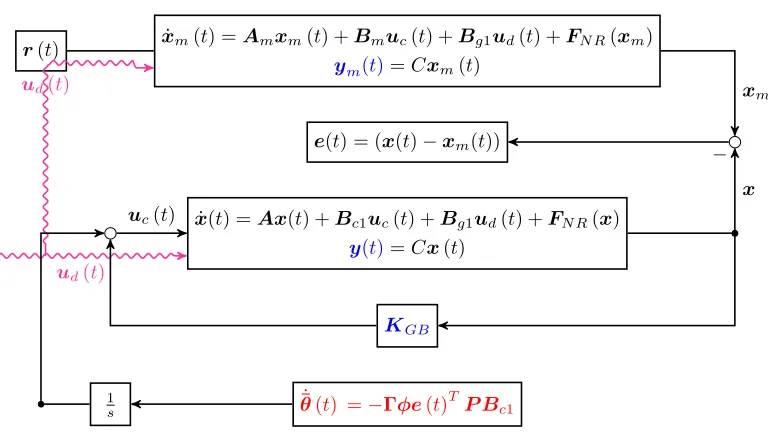
"); the terms "Simulink" and "VKTG" denote, respectively, the Von Kár-mán Wind Turbulence Model block of MATLAB and the present Von Kármán Turbulence Generator implementation, as in [142] . . . 38 2.4 Nonlinear Adaptive Control Algorithm . . . 46

3.1 Schematic of an aerofoil section with trailing-edge flap; the wind velocity is to the right and horizontal; e.a. and c.g. denote, respectively, the elastic axis and centre of gravity (from [98]) . . . 49 3.2 Point distribution for the NACA0012 aerofoil . . . 50 3.3 Comparison of the pressure distribution for NACA0012 aerofoil at

M∞=0.85 and α=1.0 deg for three point cloud densities, and

mea-surements taken from [165]. . . 51 3.4 Trace of the aeroelastic eigenvalues using the CFD as a function of the

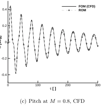
reduced velocity for a Mach number of 0.8 for the test case in Table 3.1 52 3.5 Free response comparisons using CFD and strip theory aerodynamics at

U∗

=2.0 for two Mach numbers and initial condition ξ′

(18)

3.6 CFD Response to a discrete "1–minus–cosine" gust with intensity of 1% of the freestream speed and a duration of 25 in nondimensional time, at Mach 0.8. . . 55 3.7 Free response of aerofoil model toξ′

= 0.01atU∗

= 4.6, for the reference parameters in Table 3.3 . . . 59 3.8 Full–order (FOM) and reduced–order model (ROM) eigenvalues in [rad/s∗

] 59 3.9 Response to a "1-minus-cosine" gust of intensity 5% of the freestream

speed and a length of 25 semichords atU∗

= 4.6, for the model in Table 3.3 60 3.10 Worst–case gust search at U∗

= 4.6 for a "1–minus–cosine" gust of con-stant intensity wg = 0.05, for the reduced–order model with parameters

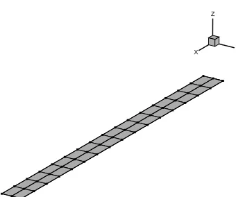
as in Table 3.3 . . . 60 3.11 Flexible wing model together with the aerodynamic sections . . . 62 3.12 Wing tip response of the HALE wing at a "1-minus-cosine" gust of

nor-malised intensity wg0 = 0.08 against MSC/NASTRAN at (U∞ = 10

[m/s] andρ∞ = 0.0899 [kg/m3]) . . . 63

3.13 Time–domain response of a free–to–pitch two–dimensional wing section; "Strip" denotes two–dimensional thin aerofoil theory (α∞ = 1.0 deg,

U∞= 50.0 m/s,h= 0.0m, and Re= 3.5·106) . . . 65

3.14 Time–domain response of a free–flying two–dimensional wing section; "Strip" denotes two–dimensional thin aerofoil theory (α∞ = 1.0 deg,

U∞= 50.0 m/s,h= 0.0m, and Re= 3.5·106) . . . 66

4.1 Open–loop and closed–loop responses for the worst–case gust for the aerofoil model in Table 3.3 . . . 70 4.2 Response to a "1-minus-cosine" gust of intensity 5% of the freestream

speed and a length of 25 semichords at U∗

= 4.6 . . . 71 4.3 Open–loop and closed–loop responses for the aerofoil with structural

non-linearities (βα3 = 2.0,βξ3 = 1.0), atU∗ = 4.6, gust intensity 5% of the freestream speed and a length of 25 semichords . . . 71 4.4 Schematic view of the experimental setup of the aeroelastic model at the

University of Liverpool . . . 72 4.5 Schematic view of the system of cables used to introduce a nonlinearity

in the wind–tunnel test–rig (from Ref. [168]) . . . 73 4.6 Structural nonlinearity in plunge displacement measured experimentally

as in Ref. [144] . . . 74 4.7 Eigenvalues tracing for varying freestream speed from simulation

per-formed here and wind–tunnel measurements taken from Ref. [101] . . . . 75 4.8 Open–loop response comparison of the linear against the nonlinear

(19)

4.10 Pitch and plunge time history of the closed–loop system for the linear controller at U = 17 m/s . . . 78

4.11 Flap response of the linear controller at U = 17 m/s . . . 79

4.12 Pitch and plunge time history of the closed–loop system atU = 17m/s with the nonlinear controller . . . 80

4.13 Flap response at U = 17 m/s of the nonlinear controller . . . 80

5.1 Schematic of a three degree–of–freedom aeroelastic system (pitch, α, plunge ξ = h/b, and flap deflection, δ), the wind velocity is to the right and horizontal . . . 83

5.2 Mode traces for validation test cases 1 and 2 . . . 85

5.3 Full model and reduced–order model basis selection at U∗

= 4.5 . . . 86

5.4 Worst–case gust search at (U∗

= 4.5) for a "1–minus–cosine" gust of in-tensity wg = 0.14 for nonlinear full and reduced model for the aerofoil case . . . 88

5.5 Aeroelastic response at (U∗

= 4.5) for the worst "1–minus–cosine" gust of intensity wg = 0.14 for nonlinear full against linear and the reduced

models for the aerofoil case . . . 89

5.6 Aeroelastic response at (U∗

= 4.5) for the worst "1–minus–cosine" gust of intensity wg = 0.14 for nonlinear reduced model against the reference model selection . . . 91

5.7 Closed–loop response predictions from nonlinear reduced–order model for different adaptation rates at(U∗

= 4.5) . . . 92

5.8 Examples of high–altitude unmanned aerial vehicle (UAV); (a) RQ4 Global Hawk in flight (courtesy U.S. Air Force), and (b) the test case of this Chapter–DSTL wing . . . 95

5.9 Geometric characteristics of the aircraft test case . . . 96

5.10 Fourth bending mode of the UAV test case mapped to the aerodynamic surface . . . 97

5.11 Nonlinear static deformation for different number of elements at sea level, 0.1 Mach number and 2 degrees angle of attack . . . 98

5.12 Variation of the structural modes (a), and gust modes eigenvalues (b), with respect to the freestream speed . . . 99

5.13 Gust response of the aircraft test case (U∞ = 59 m/s, α∞ = 4 deg,

and ρ∞= 0.0789 kg/m3); (a) convergence for increasing number of

cou-pled modes, and (b) vertical gust intensity normalised by U∞ (Military

(20)

5.14 (a) Aeroelastic response for the worst "1–minus–cosine" gust of intensity 14% of the freestream speed for nonlinear full against linear and the reduced models, and (b) dynamic response for the tuned worst–case gust at (U∞= 59m/s,α∞= 4 deg, and ρ∞= 0.0789 kg/m3) . . . 102

5.15 Closed–loop response of theH∞controller for the worst–case "1–minus–

cosine" gust for nonlinear full against open–loop responses at (U∞= 59

m/s,α∞= 4 deg, and ρ∞= 0.0789 kg/m3) . . . 103

5.16 Closed–loop response of the_H∞controller for a continuous gust for

non-linear full against open–loop responses at (U∞ = 59 m/s, α∞ = 4 deg,

andρ∞= 0.0789 kg/m3) . . . 104

5.17 Ideal reference model for the _MRAC controller design compared to the open–loop response for: (a) worst–case "1–minus–cosine" gust from Fig-ure 5.14, and (b) Von Kármán turbulence model at (U∞ = 59 m/s,

α∞= 0 deg, and ρ∞= 0.0789 kg/m3) . . . 105

5.18 Closed–loop response using theMRAC controller for various adaptation gains compared to the open–loop response for the worst–case "1-minus-cosine" gust at (U∞= 59m/s,α∞= 4 deg, and ρ∞= 0.0789 kg/m3) . 107

5.19 Closed–loop response using theMRAC controller for various adaptation gains compared to the open–loop response for a continuous gust at (U∞= 59 m/s,α∞= 4 deg, and ρ∞= 0.0789 kg/m3) . . . 108

6.1 Body reference frame and vehicle deformed coordinates . . . 112 6.2 Flying Hale Aircraft Geometry from Ref. [52] . . . 114 6.3 Test case 1– Present HALE aircraft model with the aerodynamic surfaces 114 6.4 Static deflections of the clamped wing for different angle of attack for

flow conditions as in Table 6.3 . . . 116 6.5 Variation of angle of attack with flight speed for vertical force equilibrium.

(σ1 = 1,σ2 = 2,dpl= 2,dHT P = 0). Current results compared to Murua

et al. [48] and Patil et al. [30] . . . 117 6.6 Wing displacement of the trimmed aircraft at 25 m/s against published

data from Patil et al. [30] . . . 118 6.7 Full trimming at 25 m/s for varying flexibility σ (dpl = 2, dHT P = 0)

from Murua et al. [48] . . . 119 6.8 Wing displacement of the trimmed aircraft at 25 m/s for varying

flexi-bilityσ. . . 119 6.9 Nonlinear static deformation for different number of elements at ρ∞ =

0.25 kg/m3_,_U

∞ = 25 m/s and an initial 3 degrees angle of attack . . . 121

6.10 Static aeroelastic deformations of linear against nonlinear structure . . . 121 6.11 Flight dynamics gust response for increasing stiffness parameter σ at

(21)

6.12 Eigenvalues of full model (circles) and reduced–order model (squares) real and imaginary part . . . 125 6.13 Full nonlinear against linear reduced–order model for a stochastic gust for

the different set of modes as in Table 6.7 at (U∞ = 25m/s,ρ∞ = 0.0889

kg/m3_{) . . . 127} 6.14 Error of nonlinear full against linear reduced–order model for a stochastic

Von Kármán gust for the different set of modes as in Table 6.7 at (U∞ = 25 m/s,ρ∞ = 0.0889 kg/m3) . . . 128

6.15 Maximum and minimum magnitude of the nonlinear flight dynamic re-sponse against the linear reduced–order model for a "1–minus–cosine" gust of 1.25 intensity with varying gust length at (U∞ = 25 m/s,

ρ∞ = 0.0889 kg/m3) . . . 130

6.16 Nonlinear flight dynamic response against the linear and the nonlinear reduced–order model for the worst–case "1–minus–cosine" gust of 1.25 intensity andtg = 5.0 s at (U∞ = 25 m/s,ρ∞ = 0.0889 kg/m3) . . . . 131

6.17 Closed loop (square) against open loop (circle) linearised system eigen-values in [rad/s] . . . 133 6.18 Open–loop against closed–loop responses of the nonlinear full order model

for different weighting functionsKc for the worst–case gust at an initial

rigid–body pitch angle of 5 degrees at (U∞ = 25 m/s, ρ∞ = 0.0889

kg/m3) . . . 135 6.19 Open–loop against closed–loop responses of the nonlinear full–order

model for different weighting functions Kc for a long gust length of tg = 25s and vertical normalised intensity of 1.25 . . . 136

(22)

(23)

List of Tables

3.1 Reference values of the pitch–plunge aerofoil model . . . 50 3.2 Computational cost summary . . . 55 3.3 Reference values of the pitch–plunge aerofoil model for the "heavy case"

(linear structure) . . . 58 3.4 Nondimensional eigenvalues of the model from Table 3.3 at U∗

L= 4.6 . . 58

3.5 Flexible wing material properties and basic geometric characteristics . . 61 3.6 Flow conditions and gust properties . . . 62 3.7 Reference values of the two–dimensional wing section . . . 64

4.1 Aeroelastic experiment parameters of the wing section–linear case . . . . 74 4.2 Aeroelastic numerical parameters representative of the wing section–Non

Linear case . . . 75 4.3 Open and closed–loop eigenvalues in [rad/s∗

] . . . 77 4.4 Feedback Gains for Pole Placement . . . 78

5.1 Model parameters for aerofoil test cases . . . 85 5.2 Nondimensional Reduced and Reference Model eigenvalues . . . 90 5.3 Unmmaned aerial vehicle geometrical characteristics . . . 96 5.4 First five modeshapes and frequencies of the UAV test case main wing in

[Hz] . . . 97 5.5 Basis of coupled eigenvalues used for the model projection. Real and

imaginary parts in [Hz] . . . 99 5.6 Reference Model Eigenvalues. Real and imaginary parts in [Hz] . . . 105 5.7 Adaptation Parameter selection . . . 106 5.8 Comparison of control performance for a discrete "1–minus–cosine" gust 109 5.9 Comparison of control performance for a stochastic gust . . . 109

6.1 HALE aircraft structural properties . . . 115 6.2 Comparison of vibration structural frequencies of the entire configuration

(24)

(25)

List of Symbols

ara1, ara2, ara3 = Rigid–body angular acceleration in x, y, z

arv1, arv2, arv3 = Rigid–body angular velocities in x, y, z

ard1, ard2, ard3 = Rigid–body rotation in x, y, z

ada1, ada2, ada3 = Aerofoil section angular acceleration in x, y, z

adv1, adv2, adv3 = Aerofoil section angular velocity inx, y, z

add1, add2, add2 = Aerofoil section rotation in x, y, z

αh = Centre of gravity to midchord distance nondimensional distance

A = Jacobian matrix of the residual R with respect to the statesw

b = Semichord

B,C = Second and third order operators in the Taylor expansion

c = Vector of location of aerofoil sections with respect to the wing span

ch = Nondimensional distance from the midchord to the flap hinge C_ξc = Critical damping in plunge, 2p

m Kξ C_αc = Critical damping in pitch,2√IαKα

Cξ, Cα = Viscous damping in plunge and pitch, respectively CL, Cm = Lift and pitch moment coefficients

cx, cy, cx = Location of aerofoil section with respect to the wing span

da1 = Aerofoil section acceleration in x

da2 = Aerofoil section acceleration in y

da3 = Aerofoil section acceleration in z

dv1 = Aerofoil section velocity in x

dv2 = Aerofoil section velocity in y

dv3 = Aerofoil section velocity in z

dd1 = Aerofoil section deformation inx

dd2 = Aerofoil section deformation iny

dd3 = Aerofoil section deformation inz

(26)

h = Timestep

Iα = Second moment of inertia of aerofoil about elastic axis Kξ,Kα = Plunge stiffness and torsional stiffness about elastic axis L, M = Lift and pitch moment

m = Aerofoil sectional mass

Pa, Pv, Pd = Acceleration,velocity and displacement vector P aGB = Vector of rigid–body accelerations in x, y, z P aBA = Vector of aerofoil accelerations inx, y, z P dGB = Vector of rigid–body displacements inx, y, z P dBA = Vector of aerofoil deformations in x, y, z P vGB = Vector of rigid–body velocities in x, y, z P vBA = Vector of aerofoil velocities in x, y, z ra1 = Rigid–body acceleration in x

ra2 = Rigid–body acceleration in y

ra3 = Rigid–body acceleration in z

ra = Radius of gyration of aerofoil about elastic axis, r2a = Iα/m b2 rv1 = Rigid–body velocity inx

rv2 = Rigid–body velocity iny

rv3 = Rigid–body velocity inz

rd1 = Rigid–body displacement in x

rd2 = Rigid–body displacement in y

rd3 = Rigid–body displacement in z

R = Residual vector

Rt = Rotation matrix of quaternions

Sα = First moment of inertia of aerofoil about elastic axis

Sk, Skd = Rotation matrix to body frame and its derivative

t = Physical time

U∞ = Freestream velocity

UL = Linear flutter speed U∗

= Reduced velocity,U/b ωα Uef f = Effective freestream speed

w = Vector of unknowns

wg = Gust vertical velocity

w0 = Intensity of gust vertical velocity

wf = Augmented aerodynamic states xα = Aerofoil static unbalance, Sα/m b xα = Aerofoil static unbalance, Sα/mb

(27)

Greek

α = Angle of attack

βξ3, βξ5, βα3, βα5 = Nonlinear cubic and quintic aerofoil spring constants in plunge and pitch

β, γ = Newmark integration parameters

ζξ = Damping ratio in plunge,Cξ/Cξc ζα = Damping ratio in pitch,Cα/C_αc λi =i–th eigenvalue ofA

µ = Mass ratio, m/π ρ b2

ρ = Freestream density

τ = Nondimensional time,t U/b

τg = Gust gradient

φi,ψi =i-th right and left eigenvectors ofA

ξ = Nondimensional displacement in plunge,h/b

¯

ω = Ratio ofωξ/ωα

ωα = Uncoupled pitching mode natural frequency about elastic axis,p

Kα/Iα ωξ = Uncoupled plunging mode natural frequency,

p

Kξ/m

Symbol

˙

( ) = Differentiation with respect tot,d( )/dt

( )′

= Differentiation with respect toτ,d( )/dτ

¯

(28)

Acronyms

2-DOF = Two degree–of–freedom 3-DOF = Three degree–of–freedom CFD = Computational fluid dynamics CSD = Computational structural dynamics CSM = Computational structural mechanics UVLM = Unsteady–vortex–lattice method DLM = Double–lattice–method

MPI = Message passing interface PML = Parallel meshless

RANS = Reynolds–averaged Navier–Stokes SVD = Singular value decomposition HSV = Hankel singular values FOM = Full–order model

NFOM = Nonlinear full–order model ROM = Reduced–order model

NROM = Nonlinear reduced–order model MRAC = Model reference adaptive control LQR = Linear quadratic regulator LQG = Linear quadratic Gaussian MPC = Model predictive control FL = Feedback linearisation

SOS = Sum–of–squares

UAV = Unmanned aerial vehicle HALE = High–altitude long–endurance FCS = Flight control system

(29)

Chapter 1

Introduction

The interest behind high–altitude long–endurance (HALE) vehicles has increased in re-cent years because they provide low–cost efficient platforms for a variety of applications. The low structural mass and high aerodynamic efficiency enable flight at high–altitudes and low–speeds with minimal energy consumption. The range of applications of HALE aircraft varies from monitoring and collecting data of the atmospheric environment, to rescue missions in bio-hazard poisonous environments. The advantage of unmanned HALE aircraft is their ability to operate at extreme conditions for long duration times without putting at risk human life.

The analysis and design of HALE aircraft, however, presents some unique chal-lenges that are not critical for more rigid (and stiff) aircraft. The dynamic interaction between the structural deformation of wings, the aerodynamics, and flight mechan-ics may cause structural failure as occurred in 2003 on the NASA’s Helios prototype shown in Figure 1.1. Following this accident, there was an increased interest in the aerodynamic–structural–flight response that occurs in light, very flexible and high– aspect–ratio wings [1]. The first detailed investigations into the dynamics of a very

flex-Figure 1.1: NASA Helios unmanned aerial vehicle as in Ref. [1]

[image:29.595.228.411.560.707.2]

(30)

Prior to the Daedalus Project the longest distance record by a human powered plane was set at 23 miles and took place in 1979 with a flight across the English Channel [4]. This record was broken during the initiation of the Daedalus project and as a result in 1988 Daedalus flew 73 miles over the Aegean Sea from Iraklion Air Force Base on Crete to Santorini island.

[image:30.595.184.373.392.513.2]

Helios was developed under the Environmental Research Aircraft and Sensor Tech-nology (ERAST) NASA program, as a HALE class vehicle. Two configurations were produced. The first one was tailored to achieve high–altitude and the second one was expected to achieve long–endurance flight. As expected, the first Helios configuration broke another altitude record on August13th 2001 with a flight at 96863 feet. However, the second configuration that was designed for long–endurance flight did not have the same success and on June 26th 2003 broke apart mid–flight during testing. Helios en-countered low–level turbulence during flight. After approximately 30 minutes of flight time a larger than expected wing dihedral formed because of the turbulence and the aircraft began a slowly diverging pitch oscillation. The wing dihedral remained high and the oscillations never subsided. Instead, they grew with each period and this led to the destruction of the aircraft (Figure 1.2).

Figure 1.2: NASA Helios flight accident as in [1]

One of the reasons for the Helios flight accident was the limited understanding of the fluid–structure coupling that occurs in these aircraft, and the absence of computational tools to simulate their flight behaviour under turbulence. The main aim of this thesis is the development of a multidisciplinary framework that addresses all the above issues in the analysis and design of highly flexible aircraft [5].

(31)

conditions and atmospheric turbulence of interest and are too large to be used for a careful control design.

Parametric searches are performed to estimate the critical loads that the aircraft will encounter during the expected life cycle and these are used for structural sizing. Inaccuracies in the load estimates can result in a very conservative (and inefficient) design. Thus, methods for generating reduced–order models (ROMs) via reduction of the full–order nonlinear equations of motion are needed in such a way that the essential nonlinear behaviour is preserved. The usual separation of flight dynamics and aeroelasticity is not appropriate for flight control when very low structural frequencies (which are also often associated with large amplitude motions) are present. Modelling and design methods based on a fully coupled system analysis are therefore necessary. The use of high–fidelity fluid–structure–flight models results in large order systems which are incompatible with control design as the bulk of control theory was developed for systems of relatively low–order. This introduces the question of how to reduce the dimension of the large–order nonlinear system while retaining the ability to predict nonlinear effects.

Hence, the development of a nonlinear ROM is considered in this thesis for control applications of very flexible aircraft in particular. From a simulation standpoint, the challenges to be overcome in the analysis and design of HALE aircraft are:

1. The development of a multidisciplinary framework to realistically model the non-linear interactions in the fluid, structure, flight dynamics, and control fields.

2. The lack of an approach to systematically reduce large computational models to a smaller system for faster simulation times and for control synthesis design.

3. The exploitation of advanced control design strategies to improve the effectiveness of the closed–loop response to gusts.

Several technical and scientific challenges are overcome which includes the simulation of significant aerodynamic and structural nonlinearities in the full aircraft dynamics through the systematic development of a hierarchy of fully coupled large–order models. In specific, this thesis deals with the reduction of these models to small–order nonlinear systems suitable for control development and the design of robust control laws based on these reduced nonlinear models for gust load alleviation, trajectory control and stability augmentation.

1.1 Aeroelastic Modelling of Very Flexible Aircraft

(32)

As the flexibility increases the wing deformation increases and there are additional con-tributions from the rigid body motion in the aerodynamics. Patil et al. [6] developed a formulation for the complete modelling of a HALE-type aerial vehicle. Drela [7] de-veloped an analysis tool which was implemented in ASWING, a numerical toolbox for flexible aircraft. Its formulation was based on a geometrically–exact nonlinear isotropic beam, and could provide fast analysis for flight dynamic characteristics. Other re-searchers also followed a similar approach in modelling nonlinear aeroelasticity. Cesnik and Brown designed a nonlinear structural analysis toolbox [8,9] for modelling a flexible aircraft using a strain–based approach. For example, the work presented in [9] examined a HALE–type aircraft which was modelled with a rigid fuselage and highly flexible, high– aspect–ratio composite wing representative of a very flexible aircraft (VFA). Palacios et al. [10] developed a nonlinear aeroelastic toolbox which used the three–dimensional Euler equations to model the flow, and the structural deformations were modelled using 1–D and a 2–D beam elements. Su et al. [11] presented a study on coupled aeroelas-ticity and results related to the dynamic stability and the open–loop gust responses of a blended wing–body aircraft. In that case, the wing was modelled by a low–order aeroelastic formulation that was capable of capturing the important structural nonlinear effects, and the coupling with the flight dynamics degrees–of–freedom. Aeroelastic sta-bility was assessed and compared with flutter results when all, or some of the rigid–body degrees–of–freedom were constrained.

Several researchers demonstrated the process of flexible aircraft configuration design in the past [12,13]. These investigations presented the challenges in the design of HALE type vehicles that can operate in the thin atmosphere. In particular, it was shown that the lack of methods to allow predictions of HALE structural mass, engine performance at high altitudes, and low Reynolds numbers for high–aspect–ratio configurations were challenging problems. Some of these challenges were addressed by Drela [7] who devel-oped an integrated model for aerodynamic, structural, and control simulation of flexible aircraft in extreme flight situations. The structural model was considered by including joined nonlinear beams which allowed arbitrarily large deformations.

(33)

developed numerical toolboxes, Su et al. built a very flexible UAV called the X–HALE and performed flight test [17, 18].

Palacios et al. [19] studied different type of structural dynamic models and aerody-namics in the nonlinear flight mechanics of very flexible aircraft. The structural dynamic models included displacement based, strain–based and intrinsic geometrically nonlinear beams. It was demonstrated that all the different beam finite element models could be obtained from a single set of equations. This investigation extended strain–based structural dynamic models to include shear effects. More importantly, the intrinsic first–order description of the nonlinear beam equations was found to be several times faster than conventional ones traditionally applied in the field of aeroelasticity.

In conclusion, composite beam models provide a reliable and efficient way to cap-ture the structural dynamics of high–aspect–ratio wings. Most commonly found in the literature, is the displacement and rotation–based beam formulation followed by the strain–based beam element formulation. Some work has also been published with hy-brid intrinsic geometrically nonlinear composite beams. Herein, a geometrically–exact composite beam model is used to represent the dynamics of very flexible free-flying aircraft [20]. Results are obtained using two–node displacement–based elements. In a displacement–based formulation, nonlinearities arising from large deformations are cubic terms, as opposed to an intrinsic description where they appear up to second order. This thesis addresses the nonlinear model order reduction of the developed cou-pled fluid–structure models using a high–fidelity structural modelling and low–order unsteady aerodynamics.

1.2 Unsteady Aerodynamic Model

A large variety of lower and higher–fidelity aerodynamic modelling techniques has been applied in nonlinear aeroelasticity, In multidisciplinary problems such as nonlinear aeroelasticity and very flexible aircraft (VFA) modelling, it is important to distinguish the difference between analysis methods for prediction as opposed to simulation. In a simulation, there is an increased need for a well–defined configuration for an accurate characterisation of the phenomenon in question and in these cases higher–fidelity flow modelling techniques are required. For example in aeroelasticity, a simulation may be performed in order to understand a particular fluid–structure interaction mechanism, or to establish the amplitude of a limit cycle oscillation (LCO).

(34)

The aerodynamic models range from the typical two–dimensional strip theory which is low–cost and low–fidelity, towards medium–fidelity aerodynamic models with Doublet–Lattice Method (DLM) and Unsteady Vortex–Lattice Method (UVLM) that offer relatively cheap calculations. The computational cost however increases dramati-cally with Computational–Fluid–Dynamics and this is an area that still needs advances. In this thesis, the low–fidelity aerodynamic models come from the two–dimensional

Degrees--of--Freedom

C

o

m

p

u

ta

ti

o

n

a

l

C

o

s

t

[h

]

0 75000 150000 225000 300000 0

15 30 45 60

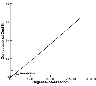
[image:34.595.192.356.225.373.2]

Potential Flow

Figure 1.3: Computational cost with respect to the degrees–of–freedom to capture 1 s of an unsteady flight dynamic calculation with strip aerodynamics and CFD

strip theory, while the higher–fidelity aerodynamics come from Computational–Fluid– Dynamics. Figure 1.3 shows the computational cost required to capture 1 s of an unsteady flight dynamic simulation with respect to the number of degrees–of–freedom with potential flow assumption and with CFD.

1.2.1 Typical Section and Strip Theory

Several analysis methods for the classical aeroelastic stability problems, divergence and flutter are available [21] since the 1930s. Of course, simplifying assumptions are made in order to reduce the complexity and the computational cost of the systems. Most simplifications address the aerodynamic part of the problem.

In the most simple case, only a representative two-dimensional section of the aeroe-lastic lifting surface (typical section) is considered reducing a three–dimensional into a two–dimensional problem which can even be analytically treated up to a certain degree. The unsteady flow is modelled in this approach by a frequency domain expression for the incompressible two–dimensional potential flow over a flat plate in harmonic motion, originally found by Theodorsen [22].

(35)

results for divergence speed, critical flutter velocity and aileron reversal. However, it requires that the physical characteristics of the configuration under investigation can be properly reduced to a beam–type structure and that three–dimensional aerodynamic ef-fects do not have a significant impact on aeroelasticity. Moreover, for high–aspect–ratio aircraft, such as very flexible aircraft flying at low cruise velocities, the two–dimensional, inviscid and incompressible unsteady aerodynamic model have been shown to predict the behaviour well. Tang et al. [23] constructed an experimental high–aspect–ratio wing aeroelastic model with a slender body at the tip. Time–domain responses due to flutter and limit cycle oscillations (LCO) were measured in a wind–tunnel test. A theoreti-cal model was developed to cross validate the experimental data. For the structural equations of motion, nonlinear beam theory was combined with the aerodynamic stall model. The theory and the experiment were in good agreement for static aeroelastic computations, flutter speed, dynamic LCO amplitude and frequency.

For the description of the non–circulatory part of the unsteady aerodynamic forces generated due to wing motion, a contribution from a gust disturbance or a control surface rotation, the idea of finite–state modelling was introduced. Wagner [24] was the first to calculate the indicial function to obtain the lift response of a two–dimensional flat plate in incompressible inviscid flow [24]. Following Wagner’s work, Jones [25] suggested the use of the Laplace transform, and also obtained an approximate expression of the Wagner function. However, there was an increased interest in the time–domain methods for the unsteady aerodynamic modelling and as a result many new modelling methods were introduced. Vepa [26] and Dowell [27] used the method of Padé approximations to give a finite–state representation of any aerodynamic frequency lift function. The newest finite–state modelling was introduced by Peters [28] who offered a new type of finite–state aerodynamic model in 1995. This model offers the finite–state equations for the induced flowfield. These equations are derived directly from the potential flow. The induced flow expansion satisfies the condition that few states will be needed in the frequency range of interest. This number of states was compared to other aerodynamic modelling techniques based on Wagner and Theodorsen functions.

One of the biggest advantages of finite–state models is that they can be cast as a small system of first–order differential equations which allows the application of control theory. Furthermore, the time evolution of the aerodynamic states is known explicitly and these can be written both in the frequency and in the time–domain.

(36)

dur-ing a gust response. Patil et al. [6, 30] coupled the geometrically–exact, intrinsic beam equations with Peters’ aerodynamics, and studied the flexibility effects on the stability of highly flexible wings with large dihedral. He concluded that their impact on the stability analysis of flexible vehicles was very important.

Very few researchers have coupled their structural solvers based on older concepts and the exponential approximations of the Wagner and Küssner functions. The Wag-ner and KüssWag-ner functions that are used in this thesis for the unsteady aerodynamic modelling, as presented in Leishman [31], have been used for the modelling of flexible free–flying aircraft with flight dynamic degrees–of–freedom [32]. Herein, additional con-tributions to the aerodynamic forces arising from the velocity and the acceleration of the control surface rotation were taken into account.

1.2.2 Doublet–Lattice Method

A large body of work has been published on the aerodynamic modelling with the Doublet–Lattice Method (DLM). DLM is based on the linearised potential flow model, solves the Laplace’s equation for the incompressible flow, and is formulated in the fre-quency domain. Moreover, it is based on the assumption of harmonic motion of lifting surfaces, which are approximated as flat plates of infinitesimal thickness. This method is combined with a structural model, usually a linear finite element model and most times an interpolation is used to define a relationship between the structural deforma-tions and the motion of the aerodynamic surfaces. DLM has been extensively used throughout the years. Blair et al. [33] provided the theoretical development of the DLM in the past 40 years. Albano et al. [34] assumed the aerodynamic surface as a set of lifting elements which were short line segments of acceleration–potential doublets. The normal velocity induced by an element of unit strength was given by an integral of the subsonic kernel function. The loads applied on each individual element were determined by assuming that they satisfied the normal velocity and the boundary conditions at a set of points on the surface. In this way he demonstrated that the DLM can be used for the calculation of lift distributions on oscillating surfaces at low speed.

(37)

very important within the range of the flight operation, and three–dimensional effects arising from the aerodynamics were minimal.

DLM underwent significant improvements during the years. Rodden et al. [39, 40] extended the aerodynamic method for applicability at higher frequencies and for flut-ter analysis, aeroservoelastic analysis of control surfaces, and short wavelength dynamic gust responses. A further refinement by Rodden et al. [40] accounted for wing tip correc-tions in the aerodynamics which resulted in an overall improvement of the convergence of the method.

Figure 1.4: Panelling scheme for an aircraft for DLM, as in [35]

The DLM is computationally inexpensive. It can model small control surface rota-tions by modifying the flow tangency boundary condition on their corresponding panels. However, the control surface aerodynamic effects obtained in this manner depend on the discretisation and usually exceed experimentally observed results, requiring empirical corrections.

1.2.3 Unsteady Vortex-Lattice Method

(38)

Katz et al. [45] was one of the first to introduce the UVLM method for the calcu-lation of the aerodynamic forces acting on lifting surfaces undergoing random three– dimensional motion. A Delta wing was considered and numerical results for high angle of attack and sideslip condition were presented. A detailed description of the method has been presented in many textbooks related to low–speed aerodynamics [46]. This technique of aerodynamic modelling makes feasible the solution of a three–dimensional potential flow based on a vortex–ring discretisation of the domain, about lifting sur-faces. These vortex–ring quadrilateral elements are used to discretise the lifting surfaces and wakes. The vorticity distribution of all vortex elements is determined by applying the non–penetration boundary condition over the bound vortex panels along the lifting surfaces.

The induced velocities over the normal vector of each individual vortex–ring are computed by the Biot–Savart law. All the inputs to the aerodynamic forces such as structural deformations, rigid–body motion, control surface rotation and gust velocities are introduced through non–vortical velocities applied on each surface panel. Following the calculation of this vorticity distribution, the aerodynamic pressures are computed using Bernoulli’s equation. The resulting aerodynamic loads are finally converted into forces and moments at the beam nodes assuming coincident meshes and rigid cross– sections [47, 48].

The UVLM is a geometrically nonlinear method in which the shape of a force–free wake is obtained as part of the solution procedure. It therefore accurately captures the aerodynamic lags over a large range of reduced frequencies at low flight velocities which makes this method suitable for the analysis of very flexible aircraft [19].

Fritz et al. [49] used the UVLM to model the oscillating plunging, pitching, twisting and flapping motions of finite–aspect ratio wings. Moreover, the results were verified by the theory and by experimental data. Palacios et al. [19] assessed different structural and aerodynamic models for the nonlinear flight dynamics of very flexible aircraft. Strip theory and Vortex–Lattice methods were considered. It was found that strip theory indicial aerodynamics perform well in small amplitude dynamics around a large static wing deflection. However, for large amplitude wing dynamics the three–dimensional aerodynamic description of UVLM gave better predictions. Murua et al. [50] studied the coupled aeroelasticity and flight mechanics of a very flexible and light vehicle that was modelled with a geometrically–exact composite beam formulation and a general three–dimensional Unsteady Vortex–Lattice Method. The stability properties and the open–loop dynamic responses of the configuration were investigated.

A typical modelling of the panelling scheme for the UVLM is shown in Figure 1.5

(39)

[image:39.595.176.446.101.315.2]

Figure 1.5: Panelling scheme for the UVLM as in [51]

1.2.4 Computational Fluid Dynamics

Computational Fluid Dynamics (CFD) is used to perform aeroelastic time–domain sim-ulations using a general model of the flow physics. Due to the relatively high cost and the need of a precise geometry definition, such simulations for fully coupled nonlinear calculations were prohibitive and have developed the last two decades.

Since the interest lies in creating the capabilities to perform a coupled fluid– structure–flight analysis, a mesh deformation tool is needed to transfer information between the fluid and the structural solver.

(40)

modelled using the three–dimensional Euler equations on a deformable mesh and static nonlinear aeroelastic calculations were performed.

Ludovic et al. [56] used the CFD solver ELSA, coupled with a simplified beam model, and computed aerodynamic calculations for static cases. Song et al. [57] presented re-sults on the aerodynamic characteristics of adaptive wings with flexible trailing–edges using the FLUENT CFD solver. It was demonstrated that during the trailing–edge de-formation the overall aerodynamic performance lift/drag ratio was increased compared to rigid trailing–edge configurations. Moreover, it was suggested that this dynamic de-flection of the wing can potentially suppress the separating stall and increase the flutter speed. Raveh et al. [58] provided two novel approaches for gust response analysis of elastic free aircraft using CFD. Furthermore, in [59] a methodology for a more computa-tionally efficient method for the gust response analysis of elastic aircraft in the transonic flight regime was introduced.

A body of work is developing for calculation based on CFD. Guo et al. [60] performed numerical simulations for discrete gust response analysis for a free–flying flexible aircraft. Trimming results and dynamic aeroelastic open–loop calculations were presented for rigid and elastic versions of a HALE–type vehicle. Kenway et al. [61] demonstrated a parallel code to perform very large calculations on multi processors for aerostructural analysis and optimisation purposes of flexible aircraft. Romanelli et al. [62] coupled a structural model with a CFD solver and computed the aeroelastic trim of a flexible free– flying aircraft. An illustration of the implementation of a multidisciplinary nonlinear Fluid–Structure Interaction (FSI) problems was presented. Sotoudeh et al. [63] dealt with gust response analysis and provided detailed studies for nonlinear beams, coupled with a hybrid quasi–steady CFD–inflow model that captured efficiently the unsteady induced gust velocity effect. Similar work was done by Hasselbring et al. [64] with the use of a linearised unsteady Reynolds averaged Navier–Stokes (URANS) code to the unsteady gust loads computation. Moreover, Ritter [65] described the CFD dynamic analysis with fully coupled structural dynamics and rigid–body dynamics. Following this, Guo et al. [66] presented a CFD based simulation for light elastic structures in maneuvering flight and Liu et al. [67] provided an efficient CFD stability analysis of flexible aircraft by the use of reduced–order models.

(41)

1.3 Model Order Reduction

Model order reduction is an active mathematical field of research that focuses on the development of low–order models to describe the dynamics of the full–order dynamic equations of a system. Reduced models can be applied in control theory [68–70], for the development of a reduced–order controller that can be implemented in a physical setup.

There is a great need for the development of reduced–order models in aeroelasticity. Firstly, they can be used in parametric studies (worst–case gust searches) and signifi-cantly speed up the computations. Secondly, because they retain the dynamics of the full–order model, they can be used directly to design a low–order controller that is applicable on the original system.

Model order reduction in structural dynamics is a well established idea. Guyan [71] provided a method to reduce the equivalent mass and stiffness matrices of large order structural dynamics systems. Han et al. [72] applied the proper orthogonal decompo-sition (POD) in the modal analysis of homogeneous structures. The model reduction method of POD was demonstrated on a detailed finite element beam model (FEM) and the resulting POD modes were compared to the theoretical modes of the beam. Kerschen et al. [73] used POD to examine the nonlinear normal modes of nonlinear structures.

In aeroelasticity, the development of reduced–order aeroelastic models has been an active area of research. Several approaches are available and have been reviewed. Lucia et al. [74] reviewed the development of reduced–order modelling techniques such as Volterra series, proper orthogonal decomposition (POD) and harmonic balance methods (HBM). Results from two–dimensional and three–dimensional test cases were presented. In Volterra series, time–domain calculations can be used to generate system responses to produce a small–order differential equation or an integral relation between the forces and the motion. Roy et al. [75] derived linear reduced–order models for systems with rigid–body degrees–of–freedom based on a component mode synthesis. Zhou et al. [69] presented a model reduction based on the balanced realisation for unstable systems.

Pioneering work in the field was published by Galerkin [76] where the proper or-thogonal decomposition (POD) method for a general equation in fluid dynamics was presented. Proper orthogonal decomposition (POD) makes use of discrete system re-sponses to provide a set of modes that can be used to reduce the full–order equations through projection.

(42)

dimensional aerofoil in unsteady motion. A discussion to extend the method to nonlinear systems was provided.

Aouf et al. [78] developed a systematic model–controller order reduction method applied to a flexible aircraft test case. This method was based on a mixed µ–synthesis to determine which flexible modes are kept in the model and found the corresponding reduced–order controller that guaranteed robust closed—loop performance. Numerical examples were given for a flexible model of a B–52 bomber and for a three–mass flexible system. Penz [79] presented three algorithms based on the common approximation of the controllability and observability grammians. The first two methods were related to the square root and the Schur method, while the third one was based on a heuristic balancing–free algorithm. The POD method was also applied on a three–dimensional nonlinear aeroelastic test case with moving boundaries in transonic flow for the AGARD 445.6 wing [80].

POD achieves a reduction in the number of spatial degrees–of–freedom. Moreover, if the aeroelastic response exhibits a periodic behaviour, then a reduction based in the time–domain can be achieved through an expansion in a Fourier series. Beran et al. [81] formulated a periodic coupled space–time solution method which was then reduced through a projection onto POD modes. However, not much has been presented on the development of nonlinear reduced–order model that can retain the full–order nonlinear dynamics behaviour.

Kim et al. [82] developed a new approach to generate CFD based ROMs for fast flutter analysis at reasonable computational cost. Samples of the unsteady response due to input commands were taken to identify the low–order matrices of the reduced sys-tem. The approach was demonstrated on a representative Boeing wind–tunnel airplane modelled with a finite element method and coupled with CFD.

Woodgate et al. [83] studied time–domain aeroelastic simulations. His approach made use of Hopf bifurcation and centre manifold theory to compute the flutter speed and the amplitude of a limit cycle oscillation (LCO). It was demonstrated that if the full– order semi–discrete system of equations is available, a nonlinear reduced–order model which is parametrised can be obtained if the nonlinear residual is first expanded in a Taylor series, and secondly is then projected onto a basis. In this way a reduced model was formed including nonlinear terms arising from high–order Jacobian–vector prod-ucts. The evaluation of these terms provided some numerical challenges but these were overcome, and a method for systematically reducing large–order aeroelastic systems to a small–order nonlinear model for LCO prediction was demonstrated.

(43)

projected onto the aeroelastic critical eigenvector. In order for the projection to be completed, matrix–free products were required which were evaluated using extended order arithmetic. This resulted in a nonlinear ordinary differential equation in one complex variable. That equation could be solved with little computational cost to ob-tain the nonlinear response of the system for chosen parameters values. Furthermore, uncertain parameters were included in the Taylor expansion, and so non–deterministic calculations for LCO response were also possible based on the reduced model. Badcock et al. [86] demonstrated all the above on a number of large dimension aeroelastic aircraft test cases.

Amsallem et al. [87] presented an interpolation method for adapting reduced–order models in aeroelasticity. He dealt with the robustness with respect to the system param-eters changes and the computational cost of the reduced–order model generation. The interpolation method was based on the Grassman manifold and its tangent space, and its applicability was demonstrated on complete fighter configurations with CFD. More-over, in [88] he dealt with the stabilisation of linear CFD based reduced–order models without affecting their accuracy. This was applied on a linearised unsteady supersonic flow, on a structural dynamics system (CSD) and on a fully coupled CSD/CFD sys-tem in the transonic flow regime. Moreover, in [89] he studied Galerkin reduced–order models for the semi–discrete wave equation. Results related to the error estimates of the approximated reduced–order model were presented. It was found that when the approximation of the POD subspace is constructed, these errors are proportional to the sum of the neglected singular values. Furthermore, in [90] a POD projection method was presented for a F–16 configuration using CFD for the subsonic, transonic and su-personic regimes. A methodology for fast, real time CFD aeroelastic computations that lies in the off–line computation of a database of reduced–order bases associated with a discrete set of flight parameters, and their corresponding interpolation method, was detailed. Another approach by the centre manifold reduction for the flutter of aero-foils under gust loading was presented in [91]. Poussot–Vassal et al. [92] presented a reduced–order model of a flexible aircraft model using Krylov methods.

Another way of model order reduction by using an ad–hoc methodology was pre-sented recently in [93] for a linear time–variant system (LTV) and the closed–loop stabilisation of a flexible wing. Model order reduction of linear time–invariant (LTI) systems is, in general a straight forward process where one has to limit the reduction error and select the stable states to be removed. Reduced–order model generation for LTV systems systems is more complex, but techniques based on coprime factorisation have been developed [68]. The main objective of the closed–loop control was to enlarge the allowable flight envelope by stabilising the flexible modes that became unstable after a certain airspeed was exceeded.

(44)

ef-fectively reduce the order of the system and thus the computational cost. Some other researchers used model order reduction techniques to derive low–order controllers for large–order aeroelastic systems and simplify the control design process [29, 95]. In this approach the order of the aircraft was reduced with balanced truncation. This was done by the use of the Hankel singular values which provide a measure of energy for each state in a system. These values form the basis for the balanced model reduction in which high energy states are retained while low energy states are discarded. Similar reduction techniques have been applied in [52,96,97] but with flight dynamics degrees–of–freedom included in the model, and potential flow assumptions.

Most of the available approaches for model order reduction deal with the deriva-tion of linear reduced–order models. One of the main contribuderiva-tions of this thesis is the development of nonlinear parametrised ROMs with respect to the induced gust ve-locity and control surface rotation and in some cases the flow conditions that retain the nonlinearity of the coupled system. This has been demonstrated with a series of two–dimensional and three–dimensional test cases coupled with a variety of lower and higher–fidelity aerodynamic solvers whose development was part of this thesis [98–103].

1.4 Control of Flexible Aircraft

The performance of very flexible aircraft can be improved by the use of active control methodologies, which makes feasible the design of lighter and larger vehicles. The objective of such an implementation is the reduction of the gust loads, the trajectory control and the stability augmentation which are achieved through feedback control, whereby actuators apply forces to the airframe based on the structural response as measured by sensors.

Control of flexible aircraft is a multidisciplinary research topic that requires tools for aerodynamic and structural dynamics and knowledge of control theory. Due to the large–order of the coupled systems, most of the time, flight control design is very challenging. The solution to that problem can come with the development of suitable reduced–order models (ROMs), so that the control system designed on the basis of the reduced model will perform well when applied to the actual distributed system. Several control approaches exist in the literature suitable for linear and nonlinear systems.

(45)

Aouf et al. [78] presented a systematic model order reduction method applied to the control of a flexible aircraft. The method was based on the µ synthesis and deter-mined which flexible modes can be truncated from the full–order model of the aircraft and found a corresponding reduced–order controller that preserved robust closed–loop performance. Numerical examples were given for a B–52 bomber and for a three–mass flexible system. Sofrony et.al [93] addressed the problem of the active mode stabilisation for an aircraft with flexible wings. The main objective of the closed–loop implementa-tion was to enlarge the allowable flight envelope (flutter speed), and this was done by stabilising flexible modes that may become unstable after a certain speed is exceeded. In that case, the original full–order model (FOM) had a large state dimension and hence a controller was designed based on the reduced–order model (ROM).

Nonlinearities in aeroelastic systems induce pathologies such as LCO under certain circumstances, and there has been limited study of the active control of these nonlin-ear aeroelastic systems. A linnonlin-ear controller usually can stabilise the nonlinnonlin-ear system but empirical evidence suggests that stability is not guaranteed in strongly nonlinear regimes. Strganac et al. [107] designed a nonlinear controller based on partial feedback linearisation. The approach followed, depended on the exact cancellation of the non-linearity. Finally, an adaptive control method was introduced in which guarantees of stability were studied both mathematically and numerically.

Nevertheless, in a physical implementation whether the system is linear or nonlinear, one needs to take into account delay effects from control surfaces and measurements of the system during the feedback loop that can potentially affect the overall stabil-ity of the system under examination. Huang et al. [108] designed a Linear Quadratic Gaussian (LQG) control that took into account such a control input delay, and demon-strated the approach on an experimental wing–tunnel model for flutter suppression. The method presented, performed better than the classical feedback and conventional LQG controllers, both of which do not take into account the input time delay. The problem of the flutter suppression was also studied by Yu et al. [109] who dealt with the experimental study of the flutter control for a wind–tunnel model by using an ultrasonic motor as an actuator. The aeroservoelastic system was based on Theodorsen’s potential flow, and a sub–optimal controller was derived due to the fact that the aerodynamic states could not be measured directly.

(46)

(_PID). Dillsaver et al. [29] investigated the problem of gust load alleviation by using reduced–order models for the control design. The reduction method used the balanced truncation that is based on the Hankel singular values to derive a low–order model. Assuming stochastic continuous gust models, an_LQG controller was designed to reduce the structural deformations. Furthermore, a command tracking control system was pre-sented for the longitudinal flight, which tracked a pitch angle command in the presence of a gust disturbance. Other approaches for gust load alleviation by means of linear op-timal control were presented in [98], and in that case, anH∞controller was efficient in

alleviating the gust loads for a two degree–of–freedom aerofoil with structural nonlinear-ities. The controller was based on the reduced model and could stabilise the nonlinear system at the worst–case gust, under realistic amplitude of induced gust velocities. H∞

control based on the linear reduced–order models for the gust load alleviation has been applied also in [96] for a very flexible aircraft with a large wing dihedral.

Cook et al. [32] presented a similar approach, where the robust linear H∞ control,

combined with a linear model order reduction methodology, was investigated for the gust rejection on a large and very flexible aircraft using trailing–edge control surfaces. For the worst–case gust length, the controller was able to reduce the peak root bending moments by approximately 9%. As the gust length was increased, the controller achieved better reduction in the loading of the linear system, but it became less capable of rejecting the disturbances on the nonlinear model. Theoretical development of the nonlinear state feedback H∞ control was presented by Van der Schaft [111]. He worked on a

nonlinear state–space analog, based on the Hamilton–Jacobi equations and inequalities, with unified results on the L2 gain analysis of smooth nonlinear systems. Goman et al. [112] compared classical engineering approaches to flight control system design (FCS) with the_H∞control by using the rigid–body modes as feedback and notch and lag filters

for the structural dynamics modes.

The nonlinear coupling of the structural dynamics and the flow equations, sometimes yields significant modelling uncertainties. A lot of work has been done on the control of linear and nonlinear systems under parametric uncertainties. For example, Fradkov et al. [113] presented a passification based robust autopilot for the attitude control of a flexible aircraft under parametric uncertainty. The application of this control methodology lies in the fact that if a system is passive with respect to some output y

then it can be asymptotically stabilised by the output feedback u=₋ky where k >0. However, with a detailed high–fidelity or even a lower–fidelity flow model this is most of the time, not true.