This is a repository copy of Educational Attainment and Risk Preference.
White Rose Research Online URL for this paper: http://eprints.whiterose.ac.uk/9938/
Monograph:
Brown, S., Ortiz, A. and Taylor, K. (2006) Educational Attainment and Risk Preference. Working Paper. Department of Economics, University of Sheffield ISSN 1749-8368 Sheffield Economic Research Paper Series 2006002
[email protected] https://eprints.whiterose.ac.uk/ Reuse
Unless indicated otherwise, fulltext items are protected by copyright with all rights reserved. The copyright exception in section 29 of the Copyright, Designs and Patents Act 1988 allows the making of a single copy solely for the purpose of non-commercial research or private study within the limits of fair dealing. The publisher or other rights-holder may allow further reproduction and re-use of this version - refer to the White Rose Research Online record for this item. Where records identify the publisher as the copyright holder, users can verify any specific terms of use on the publisher’s website.
Takedown
If you consider content in White Rose Research Online to be in breach of UK law, please notify us by
Sheffield Economic Research Paper Series
SERP Number: 2006002
ISSN 1749-8368
Sarah Brown, Aurora Ortiz and Karl Taylor
Educational Attainment and Risk Preference.
February 2006.
Department of Economics University of Sheffield 9 Mappin Street Sheffield
S1 4DT
United Kingdom
Abstract:
We explore the relationship between risk preference and educational attainment for a sample of adults drawn from the 1996 U.S. Panel Study of Income Dynamics (PSID). Using a sequence of questions from the 1996
PSID, we construct measures of an individual’s risk aversion and risk tolerance allowing us to explore the
implications of interpersonal differences in risk preference for educational attainment. Our empirical findings suggest that an individual’s degree of risk aversion (tolerance) is inversely (positively) associated with their educational attainment. In addition, using the 1997 and 2002 Child Development Supplements of the PSID, we explore the relationship between the risk preference of parents and the academic achievements of their children. Our findings suggest that a parent’s degree of risk aversion (tolerance) is negatively (positively) related to the academic achievements of their children.
Key Words: Human Capital; Risk Aversion; Risk Preference
JEL Classification: J24; J30
Acknowledgements: We are grateful to the Leverhulme Trust for providing financial support, grant reference
F/00212/J. We are also grateful to the Institute for Social Research, University of Michigan for supplying the
Panel Study of Income Dynamics 1968 to 2001 and the Child Development Supplements, 1997 and 2002. We are
I. Introduction and Background
Given the uncertainty surrounding returns to investments in human capital, it is not surprising that the risk preference of individuals has played a key role in the theory of human capital accumulation.1 By definition, any investment in human capital can be considered risky, since the return is unknown and uncertain. For example, Palacios-Huerta (2003) finds that, due to the degree of risk associated with human capital investments, the actual gains from higher education per unit of risk in the U.S. are in the region of 5 to 20 per cent higher than that from risky financial assets.2 Furthermore, it is not clear how one can reduce the degree of risk associated with human capital investments. As pointed out by Shaw (1996), the standard approach to reducing risk in financial investment, namely diversification, is often not available in the context of human capital investment. Typically, an individual holds one job with his/her human capital investments tailored accordingly. Hence, given the risk associated with returns to human capital investments, as well as difficulties with the diversification of such investments, the risk preference of individuals plays an important role in the decision to acquire human capital.
Given the obvious problems in measuring individuals’ risk preferences, it is not surprising that attitudes towards risk have attracted limited attention in the empirical literature. In some empirical models of human capital accumulation, a parameter of constant risk aversion has been included,3 but such an approach does not allow variation in risk preferences across individuals to play a role in the investment decision-making process. Belzil and Hansen (2004), for example, estimate a dynamic programming model of schooling decisions where the degree of risk aversion is inferred from school decisions. In this model,
1
See, for example, Johnson (1978), Levhari and Weiss (1974) and Gibbons and Murphy (1992).
2
Harmon et al. (2003a) have adjusted the returns to schooling for individual risk by estimating Mincerian wage equations allowing for random coefficients, which yields dispersion (i.e. risk) in the returns to schooling by assigning individual specific returns.
3
individuals are assumed to be heterogeneous with respect to ability yet homogenous with respect to the degree of risk aversion.
An important exception in the literature is Shaw (1996) who jointly models investment in risky human capital and financial wealth allowing for interpersonal differences in risk preference. Shaw (1996) presents a theoretical framework which predicts an inverse relationship between an individual’s degree of risk aversion and investment in risky human capital. The model is based on a portfolio allocation framework extended to incorporate an individual’s decision to invest in risky human capital. Since human capital accumulation is modeled as a standard investment process, the less risk averse individuals are predicted to invest in relatively high levels of education. The empirical analysis suggests that risk preference affects the returns to human capital, although the relationship between risk preference and educational attainment is not directly explored. Brown and Taylor (2005) find supporting evidence using British panel data. In a similar vein, Brunello (2002) presents a theoretical framework which predicts that risk aversion affects educational choice via the marginal utility of schooling. The theoretical framework predicts that selected years of schooling decrease when absolute risk aversion increases. The empirical findings, which are based on Italian household survey data, support the theoretical priors. This result has received further recent empirical support from Guiso and Paiello (2007). Belzil and Leonardi (2007) also use Italian survey data to explore whether the transition from different levels of education changes with risk aversion and parental education background. Their findings suggest that different attitudes towards risk do not determine the level of schooling.
In a similar vein, Barsky et al. (1997) present measures of preference parameters relating to risk tolerance, time preference and inter-temporal substitution based on the U.S.
Health and Retirement Study. The authors explore how risk preference varies across
completed and risk tolerance. Individuals with twelve years of schooling were found to be the least risk tolerant, whilst individuals with more than sixteen years of schooling were found to have greater than average risk tolerance. In the multivariate regression analysis, however, the findings suggest that years of schooling are not associated with risk preference. It should be acknowledged that intuitively one might argue that a risk averse individual may have an incentive to invest heavily in human capital in order to safe-guard his/her future. Belzil and Hansen (2004) find that a counterfactual increase in risk aversion increases educational attainment, i.e. human capital accumulation.
In sum, the relationship between risk preference and educational attainment has attracted attention in both the empirical and the theoretical literature on human capital accumulation. According to such arguments, educational attainment (i.e. human capital accumulation) is influenced by risk preference. Our paper contributes to this area – specifically we further explore the relationship between risk preference and human capital accumulation from an empirical perspective exploiting a measure a risk preference elicited from individuals’ responses to a hypothetical gamble. In addition, we explore the relationship between a parent’s risk preference and the academic achievements of their offspring. Given the important role that parents play in decisions regarding their children’s education, such an intergenerational link, which to our knowledge has not attracted attention in the previous empirical literature, may unveil an additional determinant of children’s educational attainment.
II. Data
Research, University of Michigan. The PSID 1996 Survey includes a Risk Aversion Section, which contains detailed information on individuals’ attitudes towards risk. The Risk Aversion Section contains five questions related to hypothetical gambles with respect to lifetime income.
To be specific, all heads of household were asked the following question (M1):
Suppose you had a job that guaranteed you income for life equal to your current total income.
And that job was (your/your family’s) only source of income. Then you are given the
opportunity to take a new, and equally good, job with a 50-50 chance that it will double your
income and spending power. But there is a 50-50 chance that it will cut your income and
spending power by a third. Would you take the new job?4 The individuals who answered ‘yes’ to this question, were then asked (M2): Now, suppose the chances were 50-50 that the
new job would double your (family) income, and 50-50 that it would cut it in half. Would you
still take the job? Those individuals who answered ‘yes’ to this question were then asked
(M5): Now, suppose that the chances were 50-50 that the new job would double your (family)
income, and 50-50 that it would cut it by 75%. Would you still take the new job? Individuals
who answered ‘no’ to Question M1 were asked (M3): Now, suppose the chances were 50-50
that the new job would double your (family) income, and 50-50 that it would cut it by 20
percent. Then would you take the job? Those individuals who replied ‘no’ were asked (M4):
Now, suppose that the chances were 50-50 that the new job would double your (family)
income, and 50-50 that it would cut it by 10 percent. Then would you take the new job?
We use the responses to this series of questions to create a six point risk aversion index, RAi as follows (the percentages of individuals in each category are also shown below):
4
% 44 . 23 % 72 . 20 % 21 . 19 % 99 . 17 % 76 . 12 % 88 . 5 4 & 3 & 1 5 4 & 3 & 1 4 3 & 1 3 2 & 1 2 5 & 2 & 1 1 5 & 2 & 1 0 ⎪ ⎪ ⎪ ⎪ ⎩ ⎪⎪ ⎪ ⎪ ⎨ ⎧ = = = = = = = = = = = = = = = = = No M No M No M if Yes M No M No M if Yes M No M if No M Yes M if No M Yes M Yes M if Yes M Yes M Yes M if RAi
Thus, the index is increasing in risk aversion such that if an individual rejects all the hypothetical gambles offered, the risk aversion index takes the highest value of 5, whilst if the individual accepts all gambles offered the risk aversion index takes the value of zero. It is interesting to note the low (high) percentage of respondents with the lowest (highest) value of the risk aversion index. Intermediate cases lie in between these two extreme values such that individuals are ranked according to their reluctance to accept the hypothetical gambles. The series of questions, thus, enables us to place individuals into one of six categories of risk aversion. Furthermore, as stated by Barsky et al. (1997), who find that this risk tolerance measure does predict risky behaviour such as smoking, drinking alcohol, not having insurance, choosing risky employment and holding risky financial assets, ‘the categories can be ranked by risk aversion without having to assume a particular form for the utility function,’ p.540.
A further measure of risk preference is available from the PSID 1996 survey based on Questions M1 to M5 above. Based on Barsky et al. (1997), a measure of risk tolerance
( ) is available in the PSID where the answers to Questions M1 to M5 have been converted
into a single quantitative index of risk tolerance, which has been corrected for measurement error.
i
RT
5
Thus, RTi being a measure of risk tolerance is inversely related to risk aversion.6
5
A detailed explanation of the conversion procedure is given by Luoh and Stafford (2005), which is summarized here. The risk tolerance data are taken from the last column of Table 1 in Barsky et al. (1997). Assume a utility function, U
( )
c =(
1/(
1−1/q)
)
c1−1/q, that q is log-normally distributed and G=ln( )
q . We observe which lies in one of the categories determined by the hypothetical gamble questions. The product of each individual’s probability of being in a particular category yields the likelihood function. Maximizing the likelihood function and computing expected means conditional on being in a particular category yields q (Luoh and Stafford, 2005).*
III. Educational and Risk preference
Our sample is restricted to those heads of household in employment in 1996 aged between 18 and 65, yielding a total of 5,277 observations.7 We explore the relationship between risk
preference and human capital accumulation by modeling education, , as a function of risk
preference:
i
e
(
i, i)
i1i f r
e = X +ε (1)
where denotes the measure of risk preference and represents a set of additional
explanatory variables, which draws on Wilson et al. (2005) and includes: age; gender;
ethnicity; the mothers’ marital status when the respondent was born; whether the respondent lived with his/her parents until age 16; whether the parents worked when the respondent was growing up; fathers’ occupational status when the respondent was growing up; number of siblings; whether the respondent was the first born; whether the mother was born outside of the U.S.; the educational attainment of both parents; type of religion and whether the family was poor when the respondent was growing up.
i
r Xi
In order to ascertain the robustness of our findings, we analyze both measures of risk preference, and . Similarly, we explore two measures of education – an index
denoting the highest educational attainment of the head of household ( ) and the number of
years of completed schooling by the head of household ( ). The highest educational
attainment variable is a five point index where: 0 denotes less than high school completed, i.e. less than grade 12; 1 denotes high school completed; 2 denotes that the individual went to college but did not graduate;
i
RA RTi
i
e
i
s
8
3 denotes that the individual graduated from college; and, finally, 4 denotes that the individual completed some postgraduate education. The number of
6
It should be re-iterated that our measures of risk preference are based on hypothetical rather than actual behavior. In Section IV, we explore an alternative measure of risk preference based on actual behavior.
7
We focus on employees given the nature of the risk aversion question in the PSID, which relates to income from employment, i.e. income from employment is explicitly stated as the only income source.
8
years of completed schooling is a continuous variable with a minimum (maximum) of 8 (17) years of schooling. We estimate equation (1) as an ordered probit model when measuring education by the index denoting the highest educational attainment of the head of household
( ) given the inherent ordering of the index. When measuring education using the number of
years of schooling completed by the head of household ( ), equation (1) is estimated by
ordinary least squares (OLS).
i
e
i
s
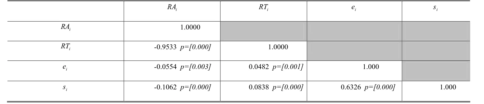
Table 1 presents a correlation matrix; between and ; between and ; and
between the risk preference and educational attainment measures. The degree of correlation between the two measures of risk preference is in accordance with a priori expectations, i.e.
the measure of risk tolerance is inversely related to the index of risk aversion. Moreover, the strong inverse relationship is significant at the one per cent level. Similarly, the correlation
between and is positive and significant at the one per cent level. Finally, the measures of
education are inversely associated with risk aversion and positively associated with risk tolerance. Such relationships between the key variables are in accordance with the empirical findings of Brown and Taylor (2005), Brunello (2002), Guiso and Paiella (2007) and Shaw (1996). Summary statistics relating to the variables used in our empirical analysis are presented in Table 2.
i
RA RTi ei si
i
e si
In Table 3 the results of estimating equation (1) are summarized for both measures of education: Panels A and B presents the results for the highest education attainment index ( )
whilst Panel C presents the results for years of completed schooling ( ). Due to the ordered
nature of the highest education attainment index ( ), we present the marginal effects of risk
preference on the probability of having each level of education from no education, i.e. less
than high school where index, , equals zero, through to having completed some
postgraduate study, where , equals four. For each measure of education, we estimate two
i
e
i
s
i
e
i
e
i
specifications: specification 1 includes in the set of explanatory variables whilst
specification 2 includes in the set of explanatory variables. The set of explanatory
variables in each of these models is as shown in Table 4, which gives the full estimation
results of the educational attainment equations where risk preference is measured by .
i
RA
i
RT
i
RA 9
It is apparent that, for our sample of 5,277 individuals, there is a statistically significant association between risk preference and both measures of education. The marginal effects show that risk preference, as measured by the risk aversion index ( ), is associated
with an increase in the probability of having less than high school education (Table 3 Panel A). Indeed, a one standard deviation increase in the risk aversion index is associated with an increase in the probability of having less than high school education by 1.9%.
i
RA
10
Similarly, at the opposite end of the educational attainment hierarchy, a one standard deviation increase in risk aversion is associated with a decrease in the probability of having completed postgraduate study by 1%. Consistent results are found with the alternative measure of educational attainment, shown in Table 3 Panel C, where increasing risk aversion is inversely
associated with the number of years of completed schooling ( ). A one point move up the
risk aversion index is associated with a decrease in the number of years of completed
schooling by around 1.9%.
i
s
11
We also consider the effect of risk tolerance ( ) upon both
measures of education. As expected, risk tolerance is inversely associated with the probability of having less than high school education (Table 3 Panel B) and correspondingly positively related to the number of years of schooling (Table 3 Panel C). For example, a one standard
i
RT
9
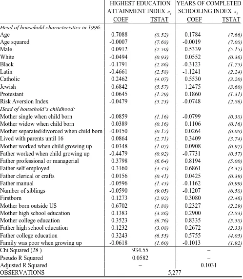
In accordance with the existing literature we find that educational attainment is increasing in: age; father’s occupation; mother’s and father’s educational attainment; religion; whether the individual is male and whether the individual was the firstborn. Factors which significantly decrease educational attainment are ethnicity and the number of siblings.
10
These calculations are based on the mean sample characteristics of individuals. For example, the 1.9% effect is calculated by multiplying the marginal effect, 0.0118, by the standard deviation of the risk aversion index, 1.6314.
11
This is calculated as a risk preference elasticity such that
(
∂ ∂ ×s r) ( )
r s , where φˆ=(
∂ ∂s r)
and r and sdeviation increase in risk tolerance is associated with a decrease in the probability of having education less than high school by 1.6% and an increase in the probability of having completed some postgraduate study by 0.9%. Noticeably, risk preference generally has a monotonic relationship with educational attainment. In general, our findings accord with those of Brunello (2002) and Guiso and Paiella (2007) in that risk aversion is found to be inversely associated with educational attainment.12
IV. Risk Preference and Time Invariance
A potential problem with our measures of risk preference is that, as argued by Brunello (2002), educational choice depends upon risk attitudes at the time of the choice rather than risk preference observed in 1996. Hence, exploring the relationship between the 1996 risk preference measures and educational attainment may be problematic as human capital investments may have been made some time ago, for instance, when the individual was at high school. The inclusion of the 1996 risk preference measures in the educational attainment equation may be appropriate if risk preferences do not vary over time or if the human capital investments were made in 1996. The extent of the time variance issue may depend on the gap between the age of the individual in 1996 and the age of the individual when the human capital investment was undertaken. This potential problem was pointed out by Brunello (2002), but was not explicitly addressed in his empirical analysis of Italian survey data. Thus, the measures of risk preference are only meaningful if risk preferences are time invariant or if the influence of the time variant component of risk preference is small in terms of magnitude. In order to explore such issues, researchers have analyzed the relationship between age and proxies for risk preference such as the propensity to hold risky financial assets. Based upon
12
U.S. data, Haliassos and Bertaut (1995), for example, found the impact of an individual’s age on the decision to hold risky stocks to be statistically insignificant. More recently, Guiso et al.
(2003) have also found the share of assets held in risky stocks to be invariant with respect to age effects in a number of countries. Such findings suggest that risk preferences do not vary with age.
We explore this issue in three ways. Firstly, we analyse the significance and magnitude of age effects in the risk preference equation. Secondly, we estimate the educational attainment equations by age cohorts in order to ascertain the robustness of the influence of risk preference on education across time. Clearly, for the youngest cohort, the potential gap between 1996 and the age of the human capital accumulation, will, on average, be the smallest. Thirdly, we exploit information relating to risk preferences from previous waves of the PSID.
We firstly model our measures of risk preference ( ) conditional upon: age; age
squared; ethnicity; gender; marital status; household size, number of children in the household; and whether the individual’s home is owned outright (i.e. without a mortgage). We also control for household wealth, household labor income, household benefit income and the log expected value of the gamble,
i
r
13
as these may influence risk preference, especially if individuals misinterpret ‘income’ in the above questions M1 to M5 to include wealth. We also
include an early measure of risk preference based on actual behaviour, which is defined in detail below. These variables are all contained in the vector Z and measured at 1996. Thus, we estimate the following equation as an ordered probit regression:
(
i,ln i)
i2i g y
r = Z +ε (2)
13
To be specific: if RA=0, ev= 0.5 2
(
LY)
+ 0.5 0.25(
LY)
; if RA=1, ; if, ; if
(
)
(
= 0.5 2 + 0.5 0.5
ev LY LY
)
)
2RA= ev= 0.5 2
(
LY)
+ 0.5 0.66(
LY RA=3, ev= 0.5 2(
LY)
+ 0.5 0.8(
LY)
; if RA=4, ; finally, if(
)
(
= 0.5 2 + 0.5 0.9In order to explore the robustness of our findings, we then re-estimate our educational attainment equations replacing with a value purged from identifiable influences, defined as: ri
2 ˆi
ε , the residual from the ordered probit model, i.e. equation (2), where the risk attitudes
index is the dependent variable and the explanatory variables represent a combination of individual and household characteristics.
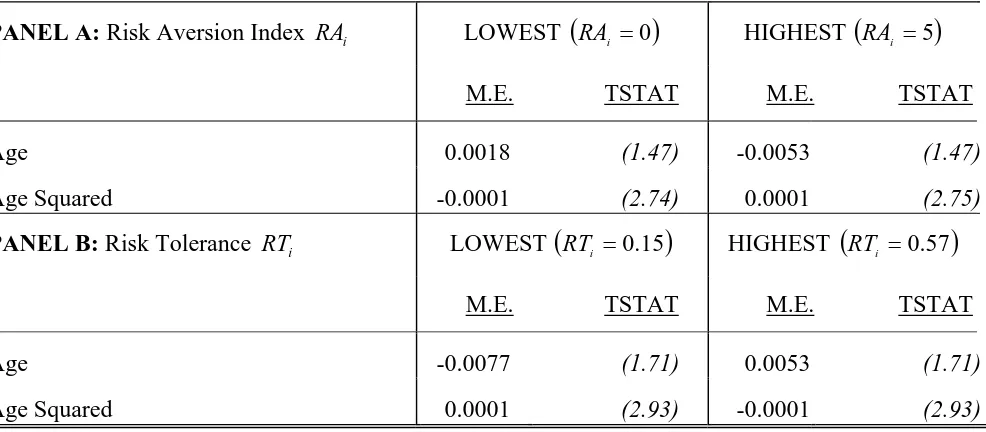
The results from estimating the two risk preference equations (i.e. risk avoidance and risk tolerance) are presented in Tables 5A and 5B. It is apparent from the estimated risk preference equations, i.e. equation (2), that and are both influenced by age which
suggests that risk preferences are not time invariant. However, the marginal effects of the quadratic in age (see Table 5B) are relatively small for both measures of risk preference at the extreme values of the two measures and are only statistically significant at the 10 per cent
level for and insignificant for .
i
RA RTi
i
RT RAi
We replicate our analysis of Table 3 by estimating equation (1) based upon εˆi2, the
residual from equation (2), for both measures of education. Table 6 Panels A and B present
the results for the highest education attainment index ( ) whilst Panel C presents the results
for years of completed schooling ( ).
i
e
i
s 14 The results summarized in Table 6 concur with those
of Table 3, where risk preference is treated exogenously, in that there is a statistically significant relationship between both measures of risk preference and education. For example,
a one standard deviation increase in εˆi2 is associated with an increase in the probability of
having less than high school education by 1%. Similarly, at the opposite end of the educational attainment hierarchy, a one standard deviation increase in εˆi2 is associated with a
decrease in the probability of having completed postgraduate study by 0.52%. Hence, our
14
Our use of a generated variable may potentially induce bias in the estimates. As such, the standard errors on 2
ˆi
findings suggest that the correlation between risk preference and education reported in Table 3 is not capturing, for example, an unobserved wealth or age effect.
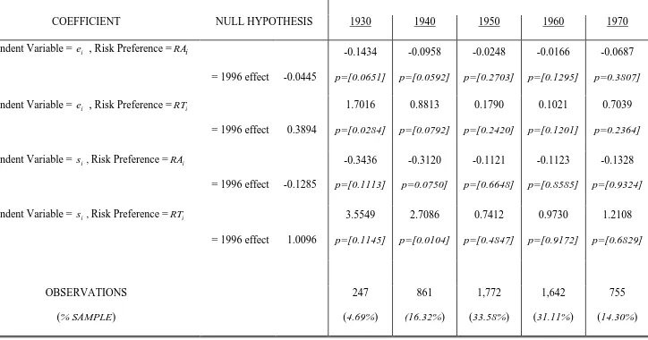
To further explore this issue, we estimate educational attainment equations by age cohorts, i.e. by individuals born in the following decades: 1930s; 1940s; 1950s; 1960s and 1970s. We test whether the influence of risk preference on educational attainment in each cohort (i.e. sub-sample) is significantly different from the estimated coefficient on risk preference in the education equation estimated over the entire sample. The results presented in Table 7 reveal that the null hypothesis that the influence of risk preference on education is the same as the 1996 effect of risk preference on education cannot, in general, be rejected across successive cohorts.15 The findings that the estimated coefficients on the risk preference measures do not vary across the age cohorts provide further support for the time invariance of the influence of risk preference on educational attainment.
Finally, over the period 1969 to 1972, an index of risk avoidance is available in four waves of the PSID, which is the early risk preference measure included in equation (2) above.
This measure of risk avoidance is derived from questions relating to factors such as the head of household’s seat belt usage, smoking behavior and purchases of medical insurance and car insurance, i.e. actual rather than hypothetical behavior. It is possible that individuals are in the sample between 1 to 4 times during the period 1969 to 1972. Hence, we take an average of the risk avoidance index over a maximum of four years as our early measure of risk preference,
. There are 647 individuals who were heads of households in both 1996 and over the
period 1969 to 1972. These individuals are aged between 41 and 65. Hence, for these individuals we can compare the relationship between the risk preference measure reported in 1996 and educational attainment with that of the risk preference measure reported over 1969
o i
RA
15
to 1972.16 Indeed, if risk preference is largely time invariant then we would expect the
relationship between and education to have the same sign and to be similar in magnitude
to that between and education. It should be explicitly acknowledged that and
do differ in terms of the underlying survey questions being based on hypothetical behavior in
the case of RA nd on actual behavior in the case of RA . Despite such differences, however, io
for this sub-sample of individuals, the correlation between the risk aversion index of 1996 and risk avoidance index of the earlier period is 0.0797, which is statistically significant at the 5 per cent level. Thus, the two risk preference variables, although constructed from survey responses given two decades apart, are positively related suggesting time invariance of risk preferences.
o i
RA
i
RA RAi RAio
i a
To further investigate the relationship between risk preference and human capital, we estimate equation (1) based on the sub-sample of 647 individuals who were present in both the 1996 PSID and at least one year in the 1969 to 1972 PSID. The results are shown in Table
8 for both measures of education: Panels A and B present the results for the highest education
attainment index ( ) for each risk measure, and Panel C presents the results for years of
completed schooling ( ). In Panels A and B, the marginal effects are reported across each of
the education categories, along with the percentage impact of a one standard deviation increase in risk preference. For this sub-sample of individuals, risk preference measured at 1996 and risk preference measured over 1969 to 1972 are both statistically significantly related to each category of educational attainment and the number of years of completed schooling. Noticeably, the association between risk preference and educational attainment is more pronounced for the earlier period relative to 1996: 6.49% versus 1.9% for the
probability of having less than high school education ( ); 7.19% versus 1% for the
i
e
i
s
0 =
i
e
16
probability of having completed some postgraduate education ( ); and 17.08% versus
1.95% for years of completed schooling. Such findings are not surprising as one might predict that the majority of educational attainment would have been achieved closer to the early time
period and, hence, the relationship between and human capital accumulation is
predictably stronger than that between risk preference measured in 1996 and educational attainment.
4 =
i
e
o i
RA
17
V. Parental Risk Preference and Children’s Academic Achievement
Given that parents play an important role in decisions regarding their children’s education, it is apparent that a parent’s risk preference may influence their off-spring’s education, potentially to a greater extent than the risk preference of the child. To be specific, an individual’s educational attainment may reflect the decisions made on his/her behalf by parents and, hence, may reflect the risk preference of the parents. In order to explore this hitherto neglected area of research, we exploit the data from the PSID Child Development
Supplement (CDS) 1997. The 1997 CDS provides additional information relating to parents in the PSID and their children with the objective being to provide information on early human capital formation.18 All PSID families with children aged between 0 and 12 were invited to complete the CDS, where up to two children per family were included in the survey. In cases where there were more than two eligible children in the family, two were randomly selected to take part in the study. Our sample of children from the 1997 CDS comprises approximately 1,000 children. We match the sample of children to the 1996 PSID, which provides detailed information on their parents, in particular, the risk preference of their parents.
17
We also explore this by including the two risk preference measures, the 1996 measure and the 1969 to 1972 measure, in the educational attainment equation simultaneously. The equality of the coefficients is always rejected at the 1 per cent level across both measures of education, with the early measure having the dominant effect.
18
We focus on the relationship between the parent’s risk preference and their children’s age-standardized scores in the Woodcock-Johnson Revised Achievement Tests, which are widely used and have been validated extensively (see Woodcock and Johnson, 1990, for further details of the tests). As part of the 1997 CDS, children aged 3 to 12 took the Woodcock-Johnson Achievement Test, covering: Reading Tests and Mathematics Test. The Reading Test is a combination of a Letter Word Identification Test and a Passage Comprehension Test; similarly, the Mathematics Test is a combination of an Applied Problems Test and a Calculation Skills Tests. Children younger that 6 years old did not complete all the tests, therefore we focus our study on the Standardized Applied Problem Test, with a sample of 1,038 children (mean age 7 years old) and the Standardized Reading Test with a sample of 722 children (mean age 9 years old).
We explore the relationship between parental risk preference and their child’s achievements in the Standardized Reading Test and the Standardized Applied Problem Test
by modeling the child’s (j) 1997 test score, TESTj, as a function of the risk preference of the
parent who is the head of household in 1996 (i) employing OLS, as follows:
(
)
1997 , 1996
j j i j
TEST =h K r +ε (3)
where denotes the measure of parental risk aversion elicited from the PSID 1996, and
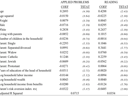
represents a set of additional explanatory variables (derived from the 1997 and 2002 CDS), which includes information related to the child such as: age; weight; gender; ethnicity; whether the child is living with his/her parents; and the number of children in the household. In this set of explanatory variables, we also include variables, which are related to the parent including: marital status; religion; years of education; household labor income, household wealth, and household income from benefits. The results presented in Table 9, Panel A, suggest that scores in the Reading and Applied Problem Tests are inversely associated with
i
the parent’s risk preference index ( ), where a one standard deviation increase in is
associated with a around a 6% (9%) lower reading (applied problem) test score. In Panel B, we replace the risk aversion index with the risk tolerance index. The results suggest that risk tolerance is positively associated with the test scores. The estimated relationship between the risk aversion/risk tolerance index and the test scores does not change when we replace the
index with its residual (
i
r RAi
2 ˆi
ε ), constructed as described above, as shown in Panels C and D.
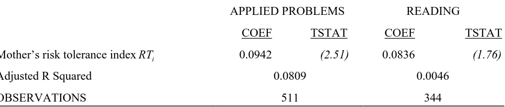
Finally, we split the sample according to whether the head of the household is the father or the mother of the child, as potentially this might influence the relationship between parental risk preference and the child’s test score. Interestingly, the results presented in Table 10, Panels A and B, suggest that the risk preference of the father has no effect on the child’s test scores. However, where the mother is the head of the household, Panels C and D, the inverse relationship between the risk aversion of the parent and the test scores of their offspring is statistically significant.
VI. Conclusions
an inverse relationship between parental risk aversion and the educational achievements of their children.
Given both the potential time and financial dimensions to the investments made by parents in their children’s education, our findings are particularly interesting from a policy-maker’s perspective. For example, our findings add to the current debate on the funding and access to higher education especially in the context of the reforms to the funding for higher education in the U.K., which have been designed to alter the social mix of students to encourage participation amongst lower socio economics groups, Greenaway and Haynes (2000). If risk-aversion is concentrated amongst the lower socio-economic groups, then our framework predicts that such individuals may be unlikely to invest in their own human capital or the human capital of their children given the current funding system.
References
Barsky, R. B., F. T. Juster, M. S. Kimball, and Shapiro, M. D. (1997). ‘Preference Parameters and Behavioural Heterogeneity: An Experimental Approach in the Health and Retirement Study.’ Quarterly Journal of Economics, 112, 537-79.
Belzil, C. and Hansen, J. (2004). ‘Earnings Dispersion, Risk Aversion and Education.’
Research in Labor Economics, 23, 335-58.
Belzil, C. and Leonardi, M. (2007). ‘Can Risk Aversion Explain Schooling Attainments? Evidence for Italy.’ Labour Economics, 14, 957-970.
Brown, J. and Rosen, S. (1987). ‘Taxation, Wage Variation, and Job Choice.’ Journal of
Labor Economics, 5, 430-51.
Brown, S. and Taylor, K. (2005). ‘Wage Growth, Human Capital and Financial Investment.’
The Manchester School, 73, 686-708.
Brunello, G. (2002). ‘Absolute Risk Aversion and the Returns to Education.’ Economics of
Education Review, 21, 635-40.
Case, A., Lubotsky, D. and Paxson, C. (2002). ‘Economic Status and Health in Childhood: The Origins of the Gradient.’ American Economic Review, 92(5), 1308-1334.
Greenaway, D. and Haynes, M. (2000). ‘Funding Universities to meet National and International Challenges.’ School of Economics Policy Report, University of Nottingham.
Guiso, L., Haliassos, M. and Jappelli, T. (2003). ‘Equity Culture: Theory and Cross-country Evidence.’ Economic Policy, 18, 123–70.
Guiso, L. and Paiella, M. (2007). ‘Risk Aversion, Wealth and Background Risk.’ Journal of
the European Economic Association. (Forthcoming).
Haliassos, M. and Bertaut, C. (1995). ‘Why Do So Few Hold Stocks?’ Economic Journal, 105, 1110–29.
Harmon, C., Hogan, V. and Walker, I. (2003a). ‘Dispersion in the Returns to Education.’
Labour Economics, 10, 205-14.
Harmon, C., Oosterbeek, H. and Walker, I. (2003b). ‘The Returns to Education: Microeconomics.’ Journal of Economic Surveys, 17, 115-55.
Johnson, W.R. (1978). ‘A Theory of Job Shopping.’ Quarterly Journal of Economics, 92, 261-78.
Levhari, D. and Weiss, Y. (1974). ‘The Effect of Risk on the Investment in Human Capital.’
American Economic Review, 61, 950-63.
Luoh, M-C. and Stafford, F. (2005). ‘Estimating Risk Tolerance from the 1996 PSID.’ http://psidonline.isr.umich.edu/data/Documentation/Cbks/Supp/rt.html
Moore, M. (1995). ‘Unions, Employment Risks, and Market Provision of Employment Risk Differentials.’ Journal of Risk and Uncertainty, 10(1), 57-70.
Murphy, K.M. and Topel, R. (1987). ‘Unemployment Risk and Earnings: Testing for Equalizing Wage Differences in the Labor Market.’ In Unemployment and the
Structure of Labour Markets, New York, NY, Basil Blackwell, 103-40.
Palacios-Huerta, I. (2003). ‘An Empirical Analysis of the Risk Properties of Human Capital Returns.’ American Economic Review, 93, 948-64.
Shaw, K. L. (1996). ‘An Empirical Analysis of Risk Aversion and Income Growth.’ Journal
of Labor Economics, 14(4), 626-53.
Weinburg, B. A. (2001). ‘An Incentive Model of the Effect of Parental Income on children.’
Journal of Political Economy, 109(2), 266-280.
Wilson, K., Wolfe, B. and Haveman, R. (2005). ‘The Role of Expectations in Adolescent Schooling Choices: Do Youths Respond to Economic Incentives?’ Economic Inquiry, 43(3), 467-92.
Woodcock, R. W. and Johnson, M. B. (1990). Woodcock-Johnson Psycho-educational
i
RA RT i ei si
i
RA 1.0000
i
RT -0.9533 p=[0.000] 1.0000
i
e -0.0554 p=[0.003] 0.0482 p=[0.001] 1.000
i
[image:22.842.36.827.69.240.2]s -0.1062 p=[0.000] 0.0838 p=[0.000] 0.6326 p=[0.000] 1.000
Table 2: Summary Statistics
MEAN STD. DEV MAX MIN
Head of household characteristics in 1996:
Highest educational attainment index ei 2.6192 1.1978 5 1
Number of years of completed schooling si 12.7998 3.1909 17 0
Risk aversion index RAi 3.1760 1.6314 5 0
Risk tolerance RTi 1.0640 1.2014 3 0
Age 39.3087 10.8307 65 18
Male 0.7218 0.4481 1 0
White 0.3945 0.4887 1 0
Black 0.2209 0.4149 1 0
Latin 0.0077 0.0878 1 0
Catholic 0.1356 0.3424 1 0
Jewish 0.1762 0.1315 1 0
Protestant 0.4508 0.4976 1 0
Log household wealth 2.11872 3.3328 14.5086 0
Log household labor income 9.5288 2.4886 13.5923 0
Log household income from benefits 0.98171 2.5546 13.8155 0
Log expected value of the gamble 13.5725 2.3914 17.5314 0
Own home 035798 0.4936 1 0
Number of children in the household 0.9840 1.1515 8 0
Household size 2.7951 1.4243 10 1
Single 0.2014 0.4011 1 0
Separated/divorced 0.2122 0.4089 1 0
Widowed 0.2899 0.1678 1 0
Head of household’s childhood:
Mother single when child born 0.4813 0.2140 1 0
Mother widow when child born 0.0036 0.0599 1 0
Mother separated/divorced when child born 0.1478 0.1206 1 0
Lived with parents until 16 0.6236 0.4845 1 0
Mother worked when child growing up 0.3213 0.4670 1 0
Father worker when child growing up 0.9990 0.0307 1 0
Father professional or managerial 0.0860 0.2804 1 0
Father self employed 0.4737 0.2124 1 0
Father clerical or crafts 0.2078 0.4058 1 0
Father manual 2.1320 3.6895 1 0
Number of siblings 2.1315 2.4935 10 0
Firstborn 0.1589 0.3657 1 0
Mother born outside US 0.2931 0.4552 1 0
Mother high school education 0.3359 0.4723 1 0
Mother college education 0.1303 03367 1 0
Father high school education 0.2141 0.4102 1 0
Father college education 0.1627 0.3692 1 0
PANEL A: HIGHEST EDUCATION ATTAINMENT INDEX (ei ) AND RISK AVERSION INDEX
LESS THAN HIGH SCHOOL COMPLETED
(ei =0)
HIGH SCHOOL COMPLETED (ei =1)
WENT TO COLLEGE DID NOT GRADUATE
(ei =2)
GRADUATED FROM COLLEGE (ei =3)
SOME POSTGRADUATE
STUDY (ei =4)
M.E. TSTAT M.E. TSTAT M.E. TSTAT M.E. TSTAT M.E. TSTAT
Risk Aversion Index RAi 0.0118 (5.22) 0.0073 (5.13) -0.0052 (5.13) -0.0076 (5.16) -0.0062 (5.16)
Chi Squared (28) 934.55 p=[0.000]
Pseudo R Squared 0.0582
PANEL B: HIGHEST EDUCATION ATTAINTMENT (ei ) AND RISK TOLERANCE
LESS THAN HIGH
SCHOOL COMPLETED (ei =0)
HIGH SCHOOL COMPLETED (ei =1)
WENT TO COLLEGE DID NOT GRADUATE
(ei =2)
GRADUATED FROM COLLEGE (ei =3)
SOME POSTGRADUATE
STUDY (ei =4)
M.E. TSTAT M.E. TSTAT M.E. TSTAT M.E. TSTAT M.E. TSTAT
Risk Tolerance RTi -0.0134 (4.39) -0.0082 (4.33) 0.0595 (4.31) 0.0086 (4.35) 0.0071 (4.35)
Chi Squared (28) 926.47 p=[0.000]
Pseudo R Squared 0.0577
PANEL C: YEARS OF COMPLETED SCHOOLING INDEX AND RISK AVERSION (si )
COEF TSTAT COEF TSTAT
Risk Aversion Index RAi -0.0748 (2.86)
Risk Tolerance RTi 0.0860 (2.44)
Adjusted R Squared 0.1079 0.1027
OBSERVATIONS 5,277
Notes: (i) Control variables are as shown in Table 4; (ii) M.E. denotes marginal effect; (iii) The results shown in Panels A and B are estimated from an ordered probit model, whilst those in
Table 4: The Determinants of Educational Attainment
HIGHEST EDUCATION ATTAINMENT INDEX ei
YEARS OF COMPLETED SCHOOLING INDEX si
COEF TSTAT COEF TSTAT
Head of household characteristics in 1996:
Age 0.7088 (8.52) 0.1784 (7.66)
Age squared -0.0007 (7.68) -0.0019 (7.08)
Male 0.0912 (2.50) 0.5339 (5.15)
White -0.0494 (0.93) 0.0552 (0.36)
Black -0.1791 (2.86) -0.3123 (1.75)
Latin -0.4661 (2.58) -1.1241 (2.24)
Catholic 0.2462 (4.07) 0.5530 (3.20)
Jewish 0.6842 (5.57) 1.2475 (3.60)
Protestant 0.0645 (1.29) 0.1860 (1.31)
Risk Aversion Index -0.0479 (5.23) -0.0748 (2.86)
Head of household’s childhood:
Mother single when child born -0.0859 (1.16) -0.0799 (0.38)
Mother widow when child born 0.0389 (0.16) 0.1106 (0.16)
Mother separated/divorced when child born -0.0150 (0.12) 0.0264 (0.08)
Lived with parents until 16 0.0864 (2.71) 0.3409 (3.74)
Mother worked when child growing up 0.0348 (1.07) 0.0908 (0.97)
Father worked when child growing up -0.4479 (0.92) -0.7731 (0.57)
Father professional or managerial 0.3798 (6.64) 0.8194 (5.00)
Father self employed 0.3160 (4.45) 0.6861 (3.37)
Father clerical or crafts 0.0156 (0.41) 0.0425 (0.39)
Father manual -0.0596 (1.45) -0.1162 (0.99)
Number of siblings -0.0590 (9.05) -0.1207 (6.58)
Firstborn 0.1273 (2.92) 0.3080 (2.46)
Mother born outside US 0.6702 (1.88) 0.2327 (2.29)
Mother high school education 0.1383 (3.86) 0.2900 (2.83)
Mother college education 0.3523 (6.76) 0.8335 (5.58)
Father high school education 0.1232 (3.08) 0.2672 (2.33)
Father college education 0.3243 (6.55) 0.5755 (4.05)
Family was poor when growing up -0.0618 (1.60) -0.1013 (1.92)
Chi Squared (28 ) 934.55 –
Pseudo R Squared 0.0582 –
Adjusted R Squared – 0.1031
OBSERVATIONS 5,277
Table 5A: The Determinants of Risk Preference
RISK AVERSION RAi RISK TOLERANCE RTi
COEF TSTAT COEF TSTAT
Age -0.0152 (1.47) 0.0193 (1.71)
Age squared 0.0003 (2.75) -0.0004 (2.93)
Male -0.2289 (5.05) 0.2423 (4.98)
White -0.0815 (1.80) 0.0577 (1.19)
Black 0.0491 (0.93) -0.0529 (0.93)
Latin -0.1850 (1.09) 0.1079 (0.59)
Single -0.1655 (2.95) 0.1939 (3.22)
Separated/divorced -0.0794 (1.47) 0.1009 (1.74)
Widow 0.0394 (0.37) 0.0456 (0.39)
Number of children in the household -0.0200 (0.64) -0.0185 (0.55)
Household size 0.2477 (0.90) 0.0042 (0.14)
Own home 0.0981 (2.71) -0.1080 (2.77)
Early risk preference measure 0.0636 (4.54) -0.0697 (4.60)
No information about early risk preference 0.0076 (0.17) -0.0171 (0.36)
Log household wealth -0.0119 (2.51) 0.0100 (1.97)
Log household labor income 0.0171 (2.73) -0.0213 (3.18)
Log household income from benefits -0.0143 (2.39) 0.0155 (2.42)
Log expected value of hypothetical gamble -0.0154 (1.54) 0.0067 (0.62)
Chi Squared (18) 281.07 p=[0.000] 237.41 p=[0.000]
Pseudo R Squared 0.0157 0.0180
OBSERVATIONS 5,277
Table 5B: The Determinants of Risk Preference – Marginal Effects of Age
PANEL A: Risk Aversion Index RAi LOWEST
(
RAi =0)
HIGHEST(
RAi =5)
M.E. TSTAT M.E. TSTAT
Age 0.0018 (1.47) -0.0053 (1.47)
Age Squared -0.0001 (2.74) 0.0001 (2.75)
PANEL B: Risk Tolerance RTi LOWEST
(
RTi =0.15)
HIGHEST(
RTi =0.57)
M.E. TSTAT M.E. TSTAT
Age -0.0077 (1.71) 0.0053 (1.71)
Age Squared 0.0001 (2.93) -0.0001 (2.93)
[image:26.595.64.557.551.767.2]PANEL A: HIGHEST EDUCATION ATTAINMENT INDEX (ei ) AND RISK AVERSION
LESS THAN HIGH SCHOOL COMPLETED
(ei =0)
HIGH SCHOOL COMPLETED
(ei =1)
WENT TO COLLEGE DID NOT GRADUATE (ei =2)
GRADUATED FROM COLLEGE (ei =3)
SOME POSTGRADUATE
STUDY (ei =4)
M.E. TSTAT M.E. TSTAT M.E. TSTAT M.E. TSTAT M.E. TSTAT
Risk Aversion Index – Residual εˆi2 0.0098 (4.32) 0.0060 (4.26) -0.0043 (4.24) -0.0063 (4.28) -0.0052 (4.29)
Chi Squared (28) 925.86 p=[0.000]
Pseudo R Squared 0.0577
PANEL B: HIGHEST EDUCATION ATTAINMENT INDEX (ei ) AND RISK TOLERANCE
LESS THAN HIGH SCHOOL COMPLETED
(ei =0)
HIGH SCHOOL COMPLETED
(ei =1)
WENT TO COLLEGE DID NOT GRADUATE (ei =2)
GRADUATED FROM COLLEGE (ei =3)
SOME POSTGRADUATE
STUDY (ei =4)
M.E. TSTAT M.E. TSTAT M.E. TSTAT M.E. TSTAT M.E. TSTAT
Risk Tolerance – Residual εˆi2 0.0540 (2.95) 0.0331 (2.93) -0.0238 (2.93) -0.0346 (2.94) -0.0286 (2.94)
Chi Squared (28) 915.87 p=[0.000]
Pseudo R Squared 0.0571
PANEL C: YEARS OF COMPLETED SCHOOLING INDEX (si )
COEF TSTAT COEF TSTAT
Risk Aversion Index – Residual εˆi2 -0.0584 (2.23)
Risk Tolerance – Residual εˆi2 -0.5423 (2.57)
Adjusted R Squared 0.1026 0.1028
OBSERVATIONS 5,277
Table 7: The Relationship between Risk Preference and Education Attainment across Age Cohorts
DECADE OF BIRTH
COEFFICIENT NULL HYPOTHESIS 1930 1940 1950 1960 1970
Dependent Variable = ei , Risk Preference =RAi
= 1996 effect -0.0445
-0.1434 p=[0.0651] -0.0958 p=[0.0592] -0.0248 p=[0.2703] -0.0166 p=[0.1295] -0.0687 p=0.3807]
Dependent Variable = ei , Risk Preference =RTi
= 1996 effect 0.3894
1.7016 p=[0.0284] 0.8813 p=[0.0792] 0.1790 p=[0.2420] 0.1021 p=[0.1201] 0.7039 p=0.2364]
Dependent Variable = si , Risk Preference =RAi
= 1996 effect -0.1285
-0.3436 p=[0.1113] -0.3120 p=0.0750] -0.1121 p=[0.6648] -0.1123 p=[0.8585] -0.1328 p=[0.9324]
Dependent Variable = si , Risk Preference =RTi
= 1996 effect 1.0096
3.5549 p=[0.1145] 2.7086 p=[0.0104] 0.7412 p=[0.4847] 0.9730 p=[0.9172] 1.2108 p=[0.6829] OBSERVATIONS (% SAMPLE) 247 (4.69%) 861 (16.32%) 1,772 (33.58%) 1,642 (31.11%) 755 (14.30%)
PANEL A: HIGHEST EDUCATION ATTAINMENT INDEX (ei ) AND RISK AVERSION (1996)
LESS THAN HIGH SCHOOL COMPLETED
(ei =0)
HIGH SCHOOL COMPLETED (ei =1)
WENT TO COLLEGE DID NOT GRADUATE
(ei =2)
GRADUATED FROM COLLEGE (ei =3)
SOME POSTGRADUATE
STUDY (ei =4)
M.E. TSTAT M.E. TSTAT M.E. TSTAT M.E. TSTAT M.E. TSTAT
Risk Aversion Index RAi 0.01949 (3.46) 0.01409 (3.33) 0.00691 (2.92) -0.01881 (3.35) -0.02167 (3.48)
Effect (%) 2.95% 2.13% 1.04% -2.84% -3.28%
Chi Squared (35) 120.62 p=[0.000]
Pseudo R Squared 0.0601
PANEL B: HIGHEST EDUCATION ATTAINMENT INDEX (ei ) AND RISK AVOIDANCE INDEX (1969-72)
LESS THAN HIGH SCHOOL COMPLETED
(ei =0)
HIGH SCHOOL COMPLETED (ei =1)
WENT TO COLLEGE DID NOT GRADUATE
(ei =2)
GRADUATED FROM COLLEGE (ei =3)
SOME POSTGRADUATE
STUDY (ei =4)
M.E. TSTAT M.E. TSTAT M.E. TSTAT M.E. TSTAT M.E. TSTAT
Risk Avoidance Index o i
RA 0.04662 (6.75) 0.03638 (6.14) 0.01888 (4.41) -0.05021 (6.21) -0.05167 (6.95)
Effect (%) 6.49% 5.06% 2.63% -6.99% -7.19%
Chi Squared (35) 166.40 p=[0.000]
Pseudo R Squared 0.0827
PANEL C: YEARS OF COMPLETED SCHOOLING INDEX (si )
COEF TSTAT Effect (%) COEF TSTAT Effect (%)
Risk Aversion Index RAi -0.25661 (4.04) 6.95%
Risk Avoidance Index RAio -0.72379 (10.67) 17.08%
OBSERVATIONS 647
Notes: (i) Control variables are as shown in Table 4; (ii) M.E. denotes marginal effect relating to the probability of having no education, i.e. less than high school; (iii) The results shown in Panels A and B are estimated from an ordered probit model, those in Panel C are from OLS estimation; (iv) in Panels A and B the “Effect (%)” figures are derived by multiplying the marginal effect by the standard deviation of the
relevant risk preference measure; (v) in Panel C the figures in the column labeled ‘Effect (%)’ are derived from
(
) ( )
Table 8: The Timing of the Measurement of Risk Preference and Educational Attainment
s r r
Table 9: Children’s Academic Test Scores and Parent’s Risk Aversion
PANEL A: DETERMINANTS OF TEST SCORES AND PARENT’S RISK AVERSION
APPLIED PROBLEMS READING
COEF TSTAT COEF TSTAT
Age 0.2693 (4.30) 0.4288 (2.43)
Age squared -0.0150 (3.64) -0.0225 (2.30)
Weight 0.0079 (3.10) 0.0045 (1.47)
Male -0.0716 (1.19) 0.0295 (0.40)
White 0.2838 (3.48) 0.2437 (2.39)
Living with parents -0.0852 (0.69) 0.1015 (0.60)
Number of children in the household -0.0236 (0.74) -0.0014 (0.04)
Parent: Single -0.2293 (1.55) 0.1046 (0.55)
Parent: Separated/divorced 0.0991 (0.68) 0.3441 (1.77)
Parent: Widow 0.0252 (0.08) 0.0760 (0.19)
Parent: Catholic 0.1246 (2.38) 0.2259 (3.45)
Parent: Jewish -0.0609 (0.28) -0.0562 (0.22)
Parent: Protestant -0.0271 (0.41) 0.0064 (0.08)
Years of education of the head of household -0.0311 (2.71) -0.0020 (0.14)
Log household labor income -0.0144 (1.12) -0.0094 (0.60)
Log household wealth 0.0043 (0.46) 0.0040 (0.35)
Log household income from benefits -0.0200 (1.65) -0.0124 (1.76)
Parent’s risk aversion index RAi -0.0322 (1.87) -0.0485 (2.00)
Adjusted R Squared 0.0715 0.0354
PANEL B: DETERMINANTS OF TEST SCORES AND PARENT’S RISK TOLERANCE
APPLIED PROBLEMS READING
COEF TSTAT COEF TSTAT
Parent’s risk tolerance index RTi 0.0521 (1.99) 0.0600 (1.88)
Adjusted R Squared 0.0727 0.0347
PANEL C: DETERMINANTS OF TEST SCORES AND PARENT’S RISK AVERSION-RESIDUAL
APPLIED PROBLEMS READING
COEF TSTAT COEF TSTAT
Parent’s risk aversion index – Residual εˆi2 -0.0330 (1.96) -0.0486 (2.00)
Adjusted R Squared 0.0716 0.0353
PANEL D: DETERMINANTS OF TEST SCORES AND PARENT’S RISK TOLERANCE -RESIDUAL
APPLIED PROBLEMS READING
COEF TSTAT COEF TSTAT
Parent’s risk aversion tolerance – Residual εˆi2 0.0258 (1.92) 0.0255 (1.81)
PANEL A: DETERMINANTS OF TEST SCORES AND FATHER’S RISK AVERSION
APPLIED PROBLEMS READING
COEF TSTAT COEF TSTAT
Father’s risk aversion indexRAi -0.0108 (0.38) -0.0347 (1.03)
Adjusted R Squared 0.0719 0.0467
PANEL B: DETERMINANTS OF TEST SCORES AND FATHER’S RISK TOLERANCE
APPLIED PROBLEMS READING
COEF TSTAT COEF TSTAT
Father’s risk tolerance indexRTi 0.0234 (0.64) 0.0401 (0.91)
Adjusted R Squared 0.0723 0.0461
OBSERVATIONS 527 378
PANEL C: DETERMINANTS OF TEST SCORES AND MOTHER’S RISK AVERSION
APPLIED PROBLEMS READING
COEF TSTAT COEF TSTAT
Mother’s risk aversion indexRAi -0.0623 (2.22) -0.0648 (1.82)
Adjusted R Squared 0.0784 0.0053
PANEL D: DETERMINANTS OF TEST SCORES AND MOTHER’S RISK TOLERANCE
APPLIED PROBLEMS READING
COEF TSTAT COEF TSTAT
Mother’s risk tolerance indexRTi 0.0942 (2.51) 0.0836 (1.76)
Adjusted R Squared 0.0809 0.0046
OBSERVATIONS 511 344
[image:31.595.62.571.484.592.2]Notes: Panels A-D contain the same control variables as given in Table 9 Panel A.